Fundamental Limits of Erasure-Coded Key-Value Stores with Side Information
Abstract
In applications of distributed storage systems to modern key-value stores, the stored data is highly dynamic due to frequent updates. The multi-version coding problem was formulated to study the cost of storing dynamic data in distributed storage systems. Previous work on multi-version coding considered a completely decentralized and asynchronous system assuming that the servers are not aware of which versions of the data are received by the other servers. In this paper, we relax this assumption and study a system where a server may acquire side information of the data versions propagated to some other servers based on the network topology. Specifically, we study a storage system with servers over a directed graph that store totally ordered versions of a message. Each server receives a subset of these versions. A server is aware of which versions have been received by its neighbors in the network graph. We show that the side information can result in a better storage cost as compared with the case where there is no side information for some regimes at the expense of the additional latency associated with exchanging the side information. Through an information-theoretic converse, we identify surprising scenarios where the side information may not help in improving the worst-case storage cost beyond the case where servers have no side information. Finally, we present a case study over Amazon web services (AWS) that demonstrates the potential cost reductions that may be obtained by our constructions.
I Introduction
00footnotetext: Ramy E. Ali (E-mail: ramy.ali@psu.edu) is with the School of Electrical Engineering and Computer Science, The Pennsylvania State University, University Park, PA and was with Nokia Bell Labs, Holmdel, NJ. Viveck R. Cadambe (E-mail: viveck@engr.psu.edu) is with the School of Electrical Engineering and Computer Science, The Pennsylvania State University, University Park. Jaime Llorca (E-mail: jaime.llorca@nokia.com) is with Nokia Bell Labs, Holmdel, NJ. Antonia M. Tulino (E-mail: a.tulino@nokia.com or antoniamaria.tulino@unina.it) is with Nokia Bell Labs, Holmdel, NJ and with the Department of Electrical Engineering and Information Technology, University of Naples Federico II, Naples, Italy. This work is supported by NSF grant No. CCF 1553248 and is published in part in the proceedings of the 2018 IEEE International Symposium on Information Theory, Vail, Colorado [1].Distributed key-value stores such as Apache Cassandra [2] and Amazon Dynamo DB [3] form an integral part of modern cloud computing infrastructure. Key-value stores are used by several applications such as reservation systems, transactions and multi-player gaming. Distributed key-value stores are engineered to deliver data with low latencies, as well as to minimize costs for the provider incurred in terms of memory and communication. Such key-value stores replicate data to ensure availability of data for a wide geographic area as well as for fault tolerance. Much research has considered reducing costs and improving latency of geo-distributed key-value stores, including various consistency models, memory management policies, and optimal data placement (See [3, 2, 4, 5, 6, 7, 8, 9, 10] and references therein).
In this paper we focus on the use of erasure coding for reducing costs of geo-distributed key-value stores by studying such systems from an information-theoretic perspective. Erasure coding is a generalization of replication that is well known to incur much lower storage costs for the same degree of fault tolerance. Although erasure coding comes at the cost of increased computational complexity for writing (encoding) and reading (decoding) data, the potential cost-savings in the face of rapidly growing data volumes has made erasure coding increasingly attractive [11, 12]. Indeed, recent research in erasure coding for distributed storage has been marked by some remarkable advances in coding theory [13, 14, 15, 16] and their implementation for archival111 1 1Archival storage systems are whose where the data does not change frequently. storage systems [17, 18].

While much research has studied erasure coding for archival storage in recent years, the study of erasure coding specifically tailored for key-value stores, which are non-archival storage systems modeled over decentralized asynchronous networks, is in its infancy. In fact, the use of erasure codes in key-value stores face some unique challenges that do not appear in archival storage. The recent works [15, 19, 20, 21, 22, 23, 24, 25, 26, 27] developed protocols that modify replication-based protocols and use erasure codes. Recall that an code - where represents the code length and represents the dimension of the code - partitions the value to be stored into data fragments and encodes them into coded fragments such that each storage node stores one coded fragment. The use of maximum distance separable (MDS) codes (e.g. Reed-Solomon codes) ensures that the value can be recovered from any of the nodes. We notice that for , there is no single node that stores the data entirely.
When such a code is used in a key-value store, when a write operation updates the data, a node has to effectively wait for a sufficient number of nodes to receive the update before deleting the old version of the data (See Fig. 1). There are two approaches to solve this problem. A common approach is to allow nodes to store older versions of data, so that in the duration of the propagation of the new version, there is indeed a coherent version of the data that can be decoded. In fact, it is demonstrated that for such key-value stores algorithms [21, 23, 20, 22, 27], each node has to store a number of versions that is linear in the degree of concurrency - the number of concurrent writes to the same object. However, the need to store older versions offsets some of the storage cost benefits of erasure coding. A second approach used by protocols [19, 24] gets around the worst case storage growth with concurrency through significantly higher communication. These protocols use message broadcast primitives where the nodes exchange data among themselves to find out the versions received by the other nodes and delete the older versions. Although these protocols store only one version of the data object per server, they can incur a significant latency especially in geo-distributed settings, as the clients have to wait for the information to propagate to large number of geographically spread out data centers before returning. Furthermore, this information exchange comes at significant communication costs, as inter-data center communication can be quite expensive.
In this paper, we depart from the previous approaches through the development of new erasure codes specifically tailored for geo-distributed key-value stores by studying them from an information-theoretic perspective. In particular, we show that conventional approaches that use standard erasure coding can be too pessimistic, and they miss opportunities to reduce the storage costs. Our coding scheme exploits the inherent network topology of the nodes storing an object, and demonstrates that exchanging some small amount of gossip information can reduce the costs incurred in erasure coding based key-value stores. Our approach can be viewed as a bridge between [23, 21, 20, 26], where no side information is exchanged among the nodes, and [19, 24] where the broadcast primitives are used to exchange complete side information among the nodes of the system2. 22 2 2We note that we mainly focus on the coding aspects and do not design an explicit protocol.
We describe the central technical contribution of our work through the multi-version coding framework [28]. Specifically, this framework abstracts out algorithmic details of key-value stores to focus on the coding-related details while retaining the essence of consistent storage systems. It thereby provides a method of developing codes for key-value stores and studying their storage costs. Achievable coding schemes for multi-version coding have been used in protocols for key-value stores in [29] and information-theoretic converses for multi-version coding have led to impossibility results that bound the costs incurred by such protocols [30]. In contrast with [28], which pessimistically assumes no side information - that is that each storage node does not know the versions received by other nodes - we assume the storage nodes can exchange meta-data information of versions received with nearby nodes, especially if the data exchange can be relatively inexpensive. The nodes that exchange this meta-data side information induce a side information graph; the vertices of the side information are the storage nodes and an edge between two nodes implies that these nodes exchange meta-data.
We determine erasure coding strategies based on the topology of the side information graph and study their storage costs. One important technical contribution we make is the identification of a graph-theoretic functional - the size of the complement of the smallest maximally externally connected subset (CSMECS) - that determines the costs of our coding strategies. We also develop information-theoretic impossibility results that bound the storage cost for a given topology. Although the central contributions of our paper are coding-theoretic in nature, we complement our results with a case study where we consider a hypothetical geo-distributed key-value store over Amazon web services (AWS). By deriving a side information graph based on the communication costs and latencies between data centers, and deriving the implied (projected) storage costs, we showcase the potential impact of our results.
II Background and Summary of Contributions
We begin with a background of quorum-based algorithms for key-value stores. We then describe the multi-version coding framework and summarize our main contributions.
II-A Quorum-based Algorithms for Consistent Key-Value Stores
We focus on key-value stores that offer simple read (get) and write (put) operations using on quorum-based algorithms. Consider a setting with storage nodes. In quorum-based protocols that use replication, e.g. the well-known ABD algorithm [31], a write operation sends a write request to all nodes and waits for the responses of at least nodes before completing the write operation, where is the write quorum size. Similarly, a read operation sends a read request to all nodes and waits for responses from at least nodes in the system before returning the value, where is the size of the read quorum.
To ensure a failure tolerance of nodes, it is required that . Key-value protocols such as [31] order the different writes333 3 3These protocols usually use Lamport clocks to order the different writes; our formulation here abstracts out these details., and require that the latest version that has propagated to at least nodes - that is, the version corresponding to latest complete write operation - can be obtained by a reader that connects to any nodes. Notice that for every pair of completed write and read operations, there are at least nodes that received the value of the write operation, and responded to the read operation. For a replication-based algorithm, and are chosen such that to ensure that the latest complete version can be obtained. The use of an MDS code with dimension would require a read operation to get data from at least nodes with the same version of the object. Thus, and are chosen such that to ensure that latest complete version can be decoded.
II-B Multi-Version Coding
The multi-version coding framework formalizes the storage strategies of key-value stores through an information-theoretic framework. Multi-version coding considers a distributed storage system of nodes that store totally ordered independent versions of a bits object. The higher ordered versions are interpreted as later versions, and lower ordered versions as earlier versions. Due to the inherent asynchrony in the system, the versions may not propagate to all the nodes. Specifically, each node receives an arbitrary subset of these versions denoting the state of that node. Any version that has been propagated to at least nodes is dubbed a complete version, and the goal at the decoder is to connect to an arbitrary subset of nodes and decode the latest complete version - the complete version with the highest order - or a later version.
For any complete version and for any set of nodes, there are at least nodes that have received that version. In the classical erasure coding model, where , the Singleton bound implies that that the storage cost per node is at least . However for , a node cannot simply store the codeword symbol corresponding to one version, since other nodes may not have received that version. In fact, the lower bound of [28] implies that the amount of information to be stored is at least . That is, there is a cost to be paid for the decentralized nature and the asynchrony in the system, and this cost grows with which intuitively corresponds to the degree of concurrency in the system. The impact of correlations has been studied in multi-version coding setting in [32]. Like all models, multi-version coding does not perfectly capture all aspects of key-value stores, yet the insights it obtains are useful. In particular, although the framework abstracts out several algorithmic issues, insights of multi-version coding have been used to develop low cost key-value store protocols [33] as well as impossibility results that bounds the cost of such protocols [30].
II-C Contributions
In this paper, we extend the scope of the multi-version coding framework, motivated by protocols such as [19, 24] where nodes exchange side information among themselves to reduce the storage cost. Our formulation is also motivated by real-world considerations of geo-distributed data stores where such data exchange can be more feasible between certain sets of nodes, depending on the topology of the nodes (data centers) and latency requirements. Specifically, we allow nodes to receive side information of the states of some other nodes based on the network topology and study the impact of this side information on the storage cost. We represent the side information by a directed graph , where an edge from vertex to vertex indicates that node is aware of the state of node .
In the completely centralized case where each node is aware of the states of all nodes, that is is a complete digraph, each node is aware of the latest complete version. In this case, a node that receives the latest complete version stores it with an MDS code of dimension . Therefore, the storage cost is . In the completely decentralized setting studied in [28], where has no edges except the self edges, the storage cost is at least . Here, we provide results that depart from the the two extreme points - the completely centralized setting where classical erasure coding-based bounds and constructions suffice, and the multi-version coding setting which is completely decentralized - and bridge the gap between them. Specifically, our contributions are as follows.
- 1.
We provide code constructions that show that this side information can reduce the worst-case storage cost significantly as compared with the case where nodes do not share their states. In particular, for a given side information graph, we identify a graph functional, that we refer to as the size of the complement of the smallest -maximally externally connected subset- or simply, the size of the -CSMECS - denoted by , which dictates the storage cost of our code constructions. Specifically, our construction has a storage cost of . In a fully connected topology, , whereas for a completely decentralized setting, is equal to . For a regular side information graph with degree , we show that , which leads to a an achievable scheme on the storage cost.
- 2.
We also provide information-theoretic lower bounds for the case of and identify a curious outcome of these results. Specifically, we identify a scenario where each node is aware of the versions received by other nodes, and yet this tremendous amount of side information does not help in improving the worst-case storage cost. These results indicate that a careful understanding of the topology is required to completely exploit the side information in distributed key-value stores.
II-D Case Study
Several services implement their own key-value stores using public cloud services, for instance, Overleaf [34] uses Amazon S3 [35]. The development of a full-fledged protocol that use our code constructions, and implementation of such a protocol is outside the scope of our work. However, we conduct a case study in Section VI-B of the potential cost savings of using our code constructions assuming a hypothetical key-value store implementation over Amazon web services public cloud. While our constructions would also be relevant for private/commercial key-value stores such as DynamoDB, the fact that the pricing information is readily available in the public cloud setting enables us to obtain a realistic understanding of the potential utility of our contributions. Current protocols either use replication [31], erasure coding that is completely decentralized [36, 20, 21, 27, 26], or assume full data exchange among the nodes and boil down to erasure coding solutions that are completely centralized [19, 24]. Based on the latencies between data centers, we construct a side information graph and calculate the size of the -CSMECS for the generated graph and show that using partial side information and our code constructions can lead to cost savings in comparison to current approaches.
Organization of the paper
The rest of this paper is organized as follows. In Section III, we formulate the multi-version coding problem with side information. In Section IV, we provide our code constructions. In Section V, we develop a lower bound on the per-server worst case storage cost. In Section VI-A, we provide numerical examples and a case study showing the storage gain of our code constructions. Finally, conclusions and future work are discussed in Section VII.
III System Model
We start with the notation. For a positive integer , we denote by the set . For any set of ordered indices , where , and for any ensemble of variables , the tuple is denoted by . We use to denote the logarithm to the base and to denote the binary entropy function. We use the notation to denote the set of -length binary strings. A code of length and dimension over alphabet consists of an injective mapping . When is a finite field and the mapping is linear, then the code is referred to as a linear code. A linear code of length and dimension is referred to as code. An linear code is referred to as maximum distance separable (MDS) if the mapping projected to any co-ordinates is invertible. In a directed graph , the in-degree of a vertex is denoted by and the out-degree of is denoted by .
We study a storage system of servers, denoted by , that can tolerate failures444 4 4By failures, we refer to servers that halt and do not respond.. The objective of the system is to store independent totally ordered versions of a message of length bits. The -th version of the message is denoted by , where . If , we interpret as a later version with respect to . The -th server receives an arbitrary subset of versions that denotes the state of that server. We denote the system state by , where denotes the power set of . In state , we denote the set of servers that have received version by .
A version that is received by at least servers is referred to as a complete version. Since the system tolerates crash failures, then is at most . A decoder that connects to an arbitrary subset of servers must obtain the latest complete version or a later version, where is at most . We provide the formal definitions next.
Definition 1.
(Complete version). In state , a complete version is a version that has been received by at least servers, that is .
The set of complete versions in state is denoted by
| (1) |
and the latest complete version is denoted by
The decoder connects to any servers and must decode a version such that .
We notice that among these servers, any complete version is present at least at servers. We assume that a server is aware of the states of some other servers in the network based on the topology. Sharing the states among the servers is specified by the side information graph that we define formally next.
Definition 2.
(Side Information Graph). The side information graph is a directed graph, where the set of the vertices represent the servers and an edge from vertex to vertex indicates that server is aware of the state of server .
Based on the side information graph, server obtains the states of some servers in the system. This set of servers is referred to as the neighborhood of server . We next define the neighborhood of server formally.
Definition 3.
(Neighborhood of server ). The neighborhood of server is the set of servers that server is aware of their states which is given by
| (2) |
We denote the states of the servers in by . The server stores a symbol from based on the versions that it receives and the local side information . We next define the multi-version code with side information formally.
Definition 4 (Multi-version code with side information).
A multi-version code with side information consists of the following
- •
encoding functions
- •
decoding functions
that satisfy the following
(3) for every possible system state , every and every set of servers , where , such that .
The objective of the multi-version coding problem is minimizing the per-server worst-case storage cost that we define next.
Definition 5 (Storage cost).
The storage cost of a multi-version code is equal to bits.
In [28], it was shown that the storage cost for the case where the versions are independent and servers do not share their states, that is , is lower-bounded as follows
| (4) |
In addition, a code construction was developed with storage cost that is given by
| (5) |
where
| (6) |
We notice that if , the storage cost of this code construction is given by
| (7) |
IV Coding With Side Information
In this section, we describe achievable schemes showing that the side information can reduce the worst-case storage cost.

We begin by explaining the intuition behind the construction as shown in Fig. 2. We intend to provide each server a methodology to distinguish between complete and incomplete versions. Once the server can identify the complete versions, it can use its storage budget on the complete versions. Note that the greater the connectivity of the graph, the more reliably a server can “guess” the set of complete versions and improve the storage cost.
Consider a state where version is complete, that is, at least servers have received . Suppose that the -th server has received version , i.e., , then this server observes through its local side information at least servers having . However, the converse may not be true. That is, there may exist an incomplete version such that a server that receives observers or more servers that receives through its side information. In particular, this can occur when that is, when the graph is incomplete555 5 5Throughout this paper, we assume that each vertex in the side information graph has a self-edge.. In our achievable strategy, a server that observes or more neighbors having version assumes that is a complete version. For any given incomplete version , the maximum number of servers that mistakenly assume that is complete is given by
| (8) |
In fact, the optimization problem in (8) can be performed over states which satisfy . In order to see this, consider two states such that . In this case, we have
Therefore, the maximum corresponds to the case where is received by exactly servers and can be simplified as follows
| (9) |
We can interpret in graph-theoretic terms as follows. In state , consider a subgraph obtained by removing all vertices corresponding to the servers that do not have an incomplete version and the corresponding edges. By definition, the out-degree of vertex in is given by
and the out-degree of in the induced graph is given by
Based on this interpretation, we can express as follows
| (10) |
In fact, the quantity motivates a graph functional that we term the size of the complement of the smallest -maximally externally connected subset of a graph (-CSMECS), that we define in Section IV-A in the context of an abstract graph . In Section IV-B, we return to the multi-version coding with side information problem and describe code constructions whose storage cost can be derived based on the size of the -CSMECS of the side information graph.
IV-A The CSMECS of a Graph
In this subsection, we develop the concept of maximally externally connected subset of a graph We use the tilde notation here to distinguish an arbitrary graph used in this subsection from the side information graph that arises in the multi-version coding problem.
Consider a directed graph . A vertex is an in-neighbor of a vertex if and an out-neighbor of if . We use to denote the set of out-neighbors and to denote the set of in-neighbors of . An induced subgraph is a subgraph of formed by a subset of the vertices and all of the edges connecting pairs of vertices in . The subgraph induced by the in-neighborhood of a vertex is called the in-neighborhood graph of and is denoted by . The subgraph induced by the out-neighborhood of a vertex is called the out-neighborhood graph of and is denoted by .
Consider a graph and any induced subgraph , where . The out-degree of any vertex is lower-bounded as follows
| (11) |
Given a subgraph , where , an -maximally externally connected subset (-MECS) is a subset of such that each vertex is connected to more than vertices outside that is in . That is, an -MECS is the set of all vertices such that each connected to every vertex outside . The -SMECS of a graph is the smallest -MECS, where the minimization is over all possible subgraphs , where .
We now define the size of the -SMECS of a graph formally.
Definition 6 (Size of the Smallest -Maximally Externally Connected Subset (-SMECS) of a Graph).
In a graph , for every integer the size of the smallest -maximally externally connected subset (-SMECS) of , , is given by
| (12) |
It is instructive to note that the size of the -SMECS of a graph does not change if the minimization in its definition is performed over all sub-graphs , where .
We denote the size of the complement of the -SMECS set by and refer to it as the -CSMECS of a graph. The -CSMECS is an important graph-theoretic quantity and dictates the storage costs of our code constructions. Note that the -CSMECS of the graph can be equivalently written as
| (13) | ||||
| (14) | ||||
| (15) |
Before we describe our constructions and associated storage costs, we give examples to illustrate the calculation of the -CSMECS of the graph for various graphs and provide some bounds. In all of our examples and throughout this paper, we assume that the vertices have self edges and we do not show them.
Example 1.
Consider the graph shown in Fig. 3, where . Consider the case where and consider a subgraph , where .
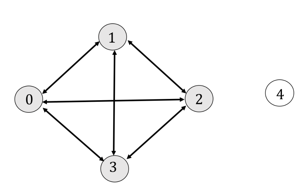
In this case, we have
and hence the -CSMECS is .
In general, determining is a discrete optimization that is computationally intractable for large graphs. We derive an upper bound on for regular directed graphs in Lemma 2. We recall that in -regular directed graph every vertex has in-degree as well as out-degree equal to . For such a graph, we have
| (16) |
We first consider the following useful lemma.
Lemma 1.
Consider any subgraph of a -regular graph , where . For any vertex a vertex , if and only if there exists at least one vertex such that .
Proof.
Consider a vertex . Suppose there exists at least one vertex , then we have
Conversely, suppose that . In this case, we have
∎
We now provide a lower bound on for -regular graphs in Lemma 2.
Lemma 2.
For any -regular graph , we have
| (17) |
Proof.
We can upper-bound as follows
where follows from Lemma 1, follows by the union bound and follows since the graph is -regular.
∎
Now, we consider the two extreme cases of the graph . The first case corresponds to a -regular graph , that is, the graph is a clique. In this case, we have
In the second case, there are no edges between the different vertices in and the graph has only self edges. In this case, we have
In Example 2, Example 3, we provide two cases of regular graphs that match the upper bound obtained in Lemma 2.
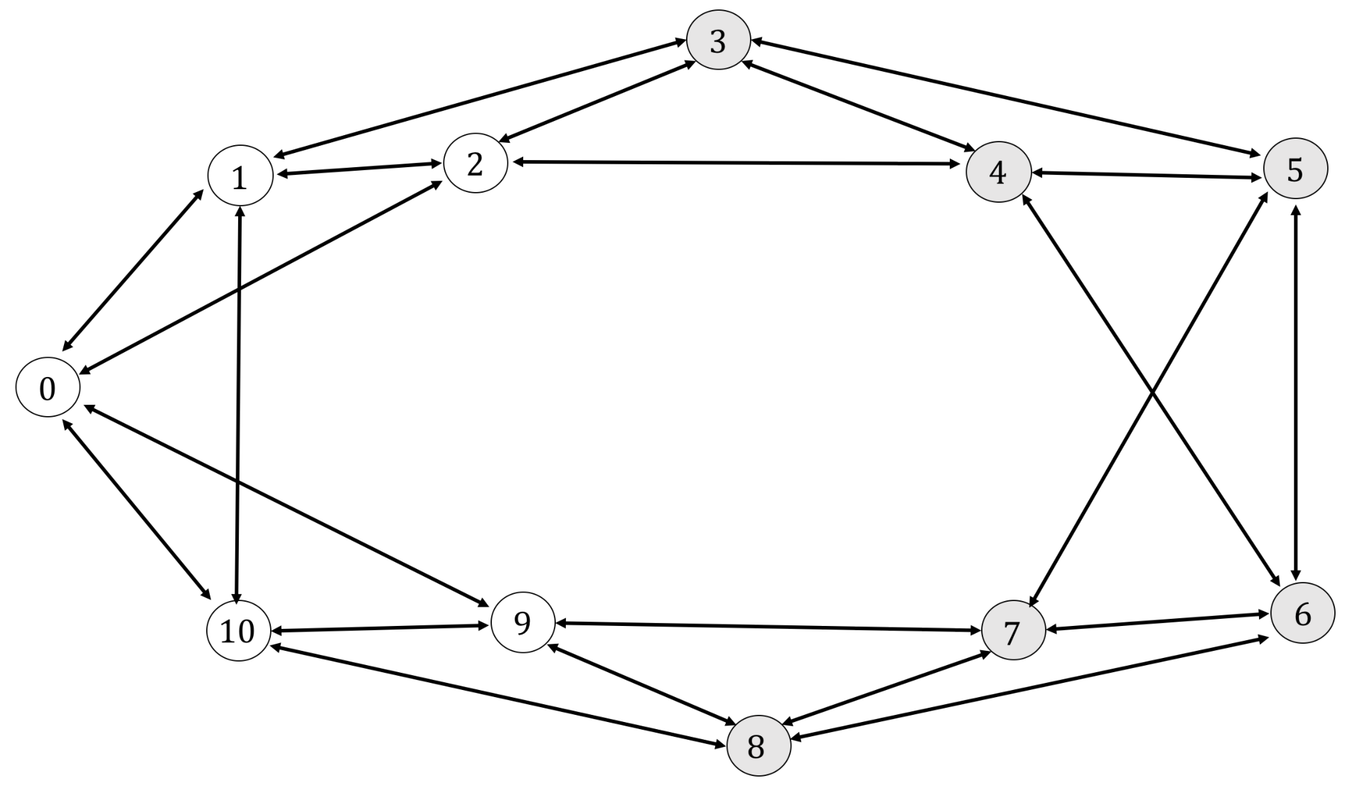
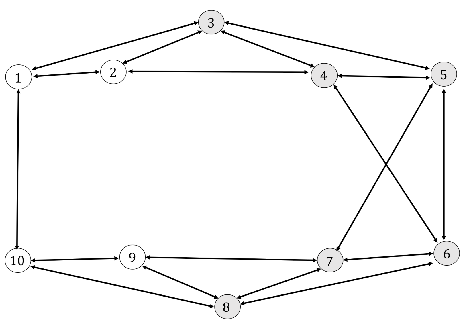
Example 2.
Consider a -regular graph , where and as shown in Fig. 4. Consider that case where and consider a subgraph , where as shown in Fig. 5. In this case, we have
and hence which matches the upper bound of Lemma 2.
Example 3.
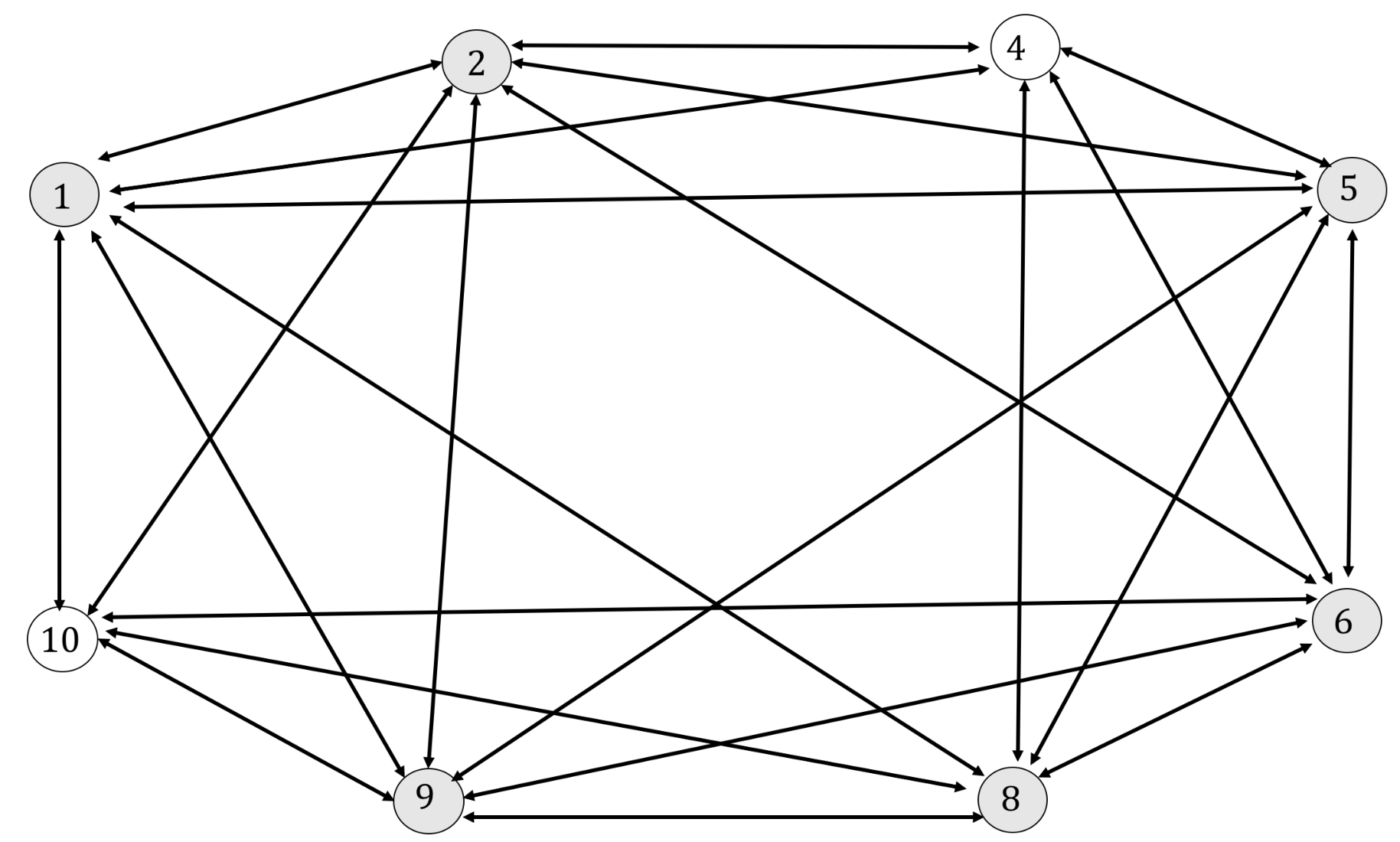
Consider a -regular graph , where and . The out-neighborhood of is given by
where the addition is modulo . Consider the case where and consider a subgraph , where as shown in Fig. 6. In this case, we have
which implies that which matches the upper bound of Lemma 2.
IV-B Code Constructions
We begin with some notations. Consider the -th server, where , and a system state . The -th server stores bits of version in this state, where . The worst-case storage cost is then given by
| (18) |
In state , we denote the latest version that server receives that is at least received by servers in the neighborhood of server by
| (19) |
We now provide our first construction. In this construction, when the -th server observes at least servers having a , it stores of . Since observing servers having does not imply that is a complete version, the -th server allocates the remaining storage budget of to as it may be the latest complete version. We provide the construction formally next.
Construction 1.
We construct a code as follows for
| (20) |
and
| (21) | ||||
| (22) |
where .
Theorem 1.
Construction 1 is a multi-version code with side information with a worst-case storage cost of
| (23) |
where .
Proof.
Consider any state . We show that the latest complete version in this state, version , is decodable. Specifically, we consider the following cases.
- •
Case (). Since , then version is incomplete. In this case, at most servers will allocate a storage budget to version . According to the construction, each of these servers will store of version and of version . Therefore, the storage allocation of version is at least
Therefore, version is decodable in this state.
- •
Case (). Since version is complete, then at least servers have it. The decoder connects to any servers. Among these servers, at least servers have received this version. Denote this set of servers by . Server observes at least servers that have received version and hence it stores of version . Since each of the servers stores of versions , then versions is decodable in this state.
∎
Remark 1.
For network topologies where , the storage cost of Theorem 1 is strictly less than and hence the side information is useful in those cases.
We next provide our second construction for any number of versions .
Construction 2.
We construct a code as follows
| (24) |
| (25) |
where and .
Theorem 2.
Construction 2 is a multi-version code with side information with a worst-case storage cost of
| (26) |
where .
Proof.
Consider any state . We show that the latest complete version in this state, version , is decodable. Specifically, we have the following cases.
- •
Consider any other version such that . Suppose that the decoder connects to any set of servers. Among these servers there are at least servers, denoted by , that have version . For any server . Therefore, for any server , we have and hence none of these servers store according to the construction.
- •
Consider any other version . Since version is incomplete, we have
A server of those servers stores of version if . Since there are at most versions that are not equal to , at least servers will store of version . Therefore, the storage allocation of version is at least
Therefore, we conclude that version is decodable in this state. ∎
Remark 2.
Remark 3.
For network topologies where , the storage cost of Theorem 2 is strictly less than and hence the side information is useful in those cases.
We compare between the case where there is no side information, the case where there is a partial side information and the complete side information case in Table V in terms of the storage cost.
| Case | Storage cost |
|---|---|
| No side information | |
| Partial side information | |
| Complete side information |
.
V Lower Bounds on the storage costs
In this section, we provide lower bounds on the storage cost. In Theorem 3, we provide a lower bound on the storage cost for any general topology that satisfies certain condition. Later on, in Theorem 4, we provide a lower bound on the storage cost for a symmetric multi-hop topology where the servers are distributed in a ring such that each server is aware of the states of its -hop neighbors.
V-A Lower bound for general topology
We begin by studying a general side information topology such that there are servers that are not aware of the states of other servers, where and . We state our result next in Theorem 3.
Theorem 3.
A multi-version code with side information where there exist servers, denoted by , such that must satisfy
| (27) |
where and .
We provide the proof of Theorem 3 in the Appendix. We next explain briefly the main idea of the proof.

The main idea of the proof follows by constructing two states and , such that and as shown in Fig. 7. Since there exist servers, denoted by , such that , then there exist servers denoted by .
We construct the two states such that servers have both versions in the two states and only servers change their states from having only in to having both versions in . In both states, the decoder connects to the same set of servers denoted by , where
. Importantly, the servers cannot differentiate between the two states as they do not know the states of the servers .
In , must be decoded as it is the latest complete version. In , the decoder can return either or as is the latest complete version. Decoding in implies that
Decoding in implies that both versions must be recoverable from the symbols of servers in and the symbols of servers in , thus
Since the decoder in this state can either decode or , we get the lower bound given by Theorem 3.
Remark 4.
For a side information graph where the set containing the possible values of has multiple values, we have
| (28) |
Corollary 1.
A multi-version code with side information where there exist two servers, denoted by , such that must satisfy
where .
The implication of Corollary 1 is that, for , if two servers are not aware of the state of one server, then the side information does not help in reducing the worst-case storage cost. That follows since a worst-case storage cost of can be achieved in a distributed manner with no side information using the code construction proposed in [28].
V-B Lower bound for a multi-hop topology
We next consider a multi-hop network topology, where the servers are distributed in a ring such that every server is aware of the states of its -hop neighbors as shown in Fig. 8.

In this topology, we denote the set of the servers by and the neighborhood of server is given by where the addition is modulo . For this topology, Theorem 4 provides an explicit lower bound on the storage cost.
Theorem 4.
A multi-version code with side information on the multi-hop topology must satisfy
| (29) |
where .
The proof of Theorem 4 follows also by constructing two states such that some servers cannot differentiate between the two states. For the case where , we have
| (30) |
Therefore, we can can apply the result obtained in Theorem 3 directly in this case. For the case where , however, the result of Theorem 3 does not apply. We present the detailed proof that handles both cases in the Appendix.
Remark 5.
For , the lower bound is given by
| (31) |
and the achievable storage cost of Theorem 1 is given by
| (32) |
Corollary 2.
A multi-version code with side information on the multi-hop topology must satisfy
| (33) |
where and .
VI Examples
In this section, we provide numerical examples showing the storage gain of our code constructions. We begin in Section VI-A by showing the storage gain for different regimes of the side information. In Section VI-B, we show the potential utility of applying our code constructions to Amazon web services (AWS).
VI-A Numerical Examples
In this subsection, we show the storage gain of our achievable schemes as compared with the storage cost of the case where there is no side information. We start with the case where we only have two versions in Example 4.
Example 4 (Multi-hop network Topology with Two Versions).
Consider a multi-hop network topology where the servers are distributed in a ring such that every server is aware of the states of its -hop neighbors. In this topology, we denote the set of the servers by and the neighborhood of server is given by where the addition is modulo . The achievable storage cost in this case is given by
In Fig. 9, we show the ratio between the storage cost of Construction 1 and the storage cost lower bound in the completely decentralized case for the case where and .
In Example 5, we show the storage gain of our scheme for the case where we have three versions.
Example 5 (Multi-hop network Topology with Three Versions).
Consider a multi-hop storage system where the servers are distributed in a ring and the system tolerates two failures. Assume that , , , hence . Fig. 10 shows the ratio between the achievable storage cost and the storage cost lower bound in the completely decentralized case for .
VI-B Case Study: Amazon Web Services
| Data center | Location | Data center | Location | Data center | Location |
| 1 | Tokyo | 6 | Frankfurt | 11 | Ohio |
| 2 | Seoul | 7 | Ireland | 12 | N. California |
| 3 | Mumbai | 8 | London | 13 | Oregon |
| 4 | Singapore | 9 | Paris | ||
| 5 | Canada | 10 | N. Virginia |
| Data center | Storage cost | Data center | Cost | Data center | Storage cost |
| 1 | 0.019 | 6 | 0.0135 | 11 | 0.0125 |
| 2 | 0.018 | 7 | 0.0125 | 12 | 0.019 |
| 3 | 0.019 | 8 | 0.0131 | 13 | 0.01 |
| 4 | 0.016 | 9 | 0.0131 | ||
| 5 | 0.0138 | 10 | 0.0125 |
.
| Data center | 1 | 2 | 3 | 4 | 5 | 6 | 7 | 8 | 9 | 10 | 11 | 12 | 13 |
| 1 | 0 | 37.8 | 157.2 | 90.8 | 177.2 | 249.7 | 234.4 | 259.4 | 259.4 | 167.5 | 166.2 | 119.6 | 106.5 |
| 2 | 37.9 | 0 | 160.1 | 105.7 | 199.7 | 269.9 | 255.7 | 269.3 | 268.2 | 190.7 | 189.3 | 153 | 128.2 |
| 3 | 136.9 | 181.5 | 0 | 68.8 | 212.8 | 129.9 | 134.4 | 128 | 118.3 | 187.7 | 202.2 | 240.8 | 225 |
| 4 | 90 | 112.4 | 82.3 | 0 | 240.9 | 189.7 | 186.4 | 181.3 | 178.5 | 267.8 | 232.6 | 184.7 | 194.7 |
| 5 | 159.2 | 189.5 | 202 | 222.3 | 0 | 103.1 | 81.7 | 92 | 95.4 | 17.8 | 27.2 | 82 | 81.7 |
| 6 | 241.3 | 267.3 | 115.3 | 174.8 | 107 | 0 | 24.2 | 19.1 | 12.8 | 90.4 | 98.9 | 147.8 | 165.4 |
| 7 | 230 | 258.4 | 128.4 | 180 | 85.2 | 23.8 | 0 | 14.6 | 21.6 | 72.7 | 84.6 | 152.8 | 137.4 |
| 8 | 236.9 | 265.3 | 116.9 | 168 | 93.9 | 15.7 | 13.2 | 0 | 10.7 | 78 | 88.7 | 141.7 | 148.5 |
| 9 | 233.5 | 301.6 | 111.6 | 173 | 97.6 | 14.4 | 20.4 | 11 | 0 | 81.7 | 99.4 | 140.7 | 157.8 |
| 10 | 164.3 | 188.8 | 195.8 | 239.9 | 18.8 | 92 | 73.1 | 79.8 | 110.5 | 0 | 13.66 | 67.2 | 79.3 |
| 11 | 162.4 | 189.9 | 199.7 | 226 | 27.6 | 121.5 | 87.7 | 91.3 | 94.6 | 16.4 | 0 | 55.9 | 74.53 |
| 12 | 111.4 | 157.9 | 253.4 | 178.3 | 81.7 | 148.7 | 150.7 | 140 | 146.7 | 67.8 | 53.9 | 0 | 23.4 |
| 13 | 109.8 | 139.7 | 226 | 166.5 | 73.4 | 167.8 | 137.8 | 150.8 | 160.4 | 84 | 73 | 25.8 | 0 |
In this subsection, we show the potential utility of applying our schemes to the data centers of Amazon. Table II and Table III provide the data centers locations and the storage prices obtained from [37] as of 03/11/2019. In Table IV, we provide the latency between data center of Amazon obtained from [38] as of 03/11/2019. We assume that a shared object is stored over the data centers , and , thus .
We note that exchanging the side information comes with a latency increase for write operations, as the data centers need to wait to hear from other data centers about the versions they received before deciding what to store. By bounding the maximum allowable latency increase, we can obtain the side information graph . Specifically, an edge exists from a data center to a data center , if the latency from the -th data center to the -th data center is below a pre-specified latency bound. Here, we use the latencies based on Table IV to explore the role of our code constructions, via a trade-off between the storage costs and latencies as shown in Fig. 11. Intuitively, allowing higher latency, may add more edges to the side information graph and that can decrease which improves the storage cost.
Note that our storage costs and latencies are projected values based on Table IV. The reported latencies should be interpreted as the additional latency incurred by write operations for writing a new value that would be incurred due to the exchange of side information. The actual latency can be higher as protocols (e.g., [31, 36, 20]) have additional rounds of communication, for instance, to discern the latest logical timestamp, etc.
We now compare between the no side information case, the partial side information case and the complete side information case in terms of the additional latency due to side information exchange and the corresponding storage cost reductions.
- A.
No side information
- •
The inter-data center latency increase due to the side information exchange is equal to .
- •
The per-server storage cost in this case is given by
The storage prices in dollars of the system is given in Table III. We denote the storage price of the -th data center by , where . The total storage price denoted by is expressed as follows
and in our case .
- •
- B.
Partial side information
- •
Latency Increase: In the case where the data centers do not exchange their states (completely decentralized system), the servers do not wait before deciding what to store. In the partial side information case, the servers wait for the side information of the other servers to be received before deciding what to store. Therefore, there is a latency increase in the partial side information case as compared with the case of no side information. For the sake of example, we assume that the maximum allowable inter-data center latency increase due to side information exchange is .
- •
The per-server storage cost is given by
While a side information graph that corresponds to the complete side information case has edges - every edge between the data centers including self edges - the side information graph that corresponds to maximum allowable latency increase of has only edges. For instance, there is no edge between the Seoul data center (#2) and Frankfurt Data center (#6) in this case. In this partial side information case, using a brute-force computer search, we can verify that
Therefore, the per-server storage cost is given by
and the total storage price is equal to
Storage Gain: The lower bound on the storage cost in case of no side information implies a storage cost that is at least bits. Therefore, in the partial side information case, we get a storage gain of of our achievable scheme as compared with the optimal achievable scheme with no side information.
- •
- C.
Complete side information
- •
The inter-data center latency increase due to side information exchange has to be at least to allow all data centers to exchange their states. Thus, there is a latency increase of at least as compared with the no side information case.
- •
The per-server storage cost in bits in this case is given by
The total storage price in this case is given by
- •
We summarize the additional latency-storage trade-off in Table V.
| Case | Maximum inter-data center latency | Storage price |
|---|---|---|
| No side information | ||
| Partial side information | ||
| Complete side information |
.
VII Conclusion
In this paper, we have studied geo-distributed key-value stores where a data center can acquire side information of the data versions propagated to some other servers or data centers based on the underlying topology. We have provided code constructions showing that the exchanging this side information results in a better storage cost compared to the no side information for some regimes at the expense of the higher latency of exchanging the side information gossip messages. We have also demonstrated the potential cost reductions and latency-storage trade-off of our constructions through a case study over Amazon web services. Interestingly, our converse results identify topologies where exchanging side information gossip messages does not improve the storage cost. Designing a protocol based on our code constructions is an interesting area of future research.
Appendix A Proof of Theorem 3
Proof.
We construct two states and with different decoding requirements such that the set of servers cannot differentiate between the two states due to the limited side information. In particular, and are constructed such that only servers, denoted by change their states from to .
- 1.
State . In this state, is the latest complete version and hence it must be decoded. In particular, servers have both and and the remaining do not have any version. The set of servers that have is given by the following disjoint union
where . In this state, the decoder connects to the following set of servers
We denote the value stored at the -th server, , in this state by Since is the latest complete version in this state, we must have
(34) Thus, we have the following inequalities
(35) where follows since we assume that are independent and uniformly distributed over as the code should work for any distribution of .
- 2.
State . In this state, is the latest complete version. Therefore, the decoder can either return or . In particular, servers have both , , servers have only and the remaining servers do not have any version. The set of servers that have is given by
and the set of servers that have is given by
Suppose that the decoder connects to the following set of servers
We denote the value stored at the -th server, , in this state by . Since servers observe the same information in both states, we have , for . In this state, the decoder must either return or . We consider these cases next.
- (a)
In order to decode in this state, we must have
(36) Consequently, we have the following inequities
where follows since . Therefore, the storage cost is lower-bounded as follows in this case
(37) - (b)
In order to decode in this state, we must have
(38) Consequently, we have the following inequalities
(39) Moreover, since and and are independent, we have
. Therefore, (39) can be rewritten as follows
where the last equality follows since as those servers only have . This implies with (35) the following
Therefore, the storage cost in this case is lower-bounded as follows
(40)
Since in state the decoder can decode either or , the storage cost is lower-bounded as follows
(41) - (a)
∎
Appendix B Proof of Theorem 4
Proof.
We consider the multi-hop network and construct two states and . The two states have different decoding requirements, but the set of servers , where , cannot differentiate between the two states. To keep the notation simple, we denote by .
- 1.
State . In this state is the latest complete version. Therefore, the decoder must return in this state. The set of servers that have is the same as the set of servers that have and is given by the following disjoint union
where . The decoder connects to the following set of servers to decode
The symbol stored by the -th server in this state is denoted by , where . Since is the latest complete version in this state, we must have
(42) Therefore, we have the following inequalities
(43) - 2.
State . In this state is the latest complete version. The decoder in this case must either return or . The set of servers that have is given by
The set of servers that have is given by
The decoder connects to the following set of servers to decode either or
The symbol stored at the -th server in this state is denoted by , where . Since servers observe the same information in both states, we have , for .
Depending on which version the decoder will return, we consider the following cases.- (a)
In order to decode in this state, we must have
(44) Consequently, we have the following inequities
where follows since and . Therefore, decoding in this state implies a storage cost that is lower-bounded as follows
(45) - (b)
In order to decode in this state, we must have
Consequently, we have the following inequalities
(46) Since and are independent, we also have
(47) . Therefore, we have
where the last equality follows as since those servers only have received . This implies with (43) the following
Therefore decoding implies a storage cost that lower-bounded as follows
(48)
Since in state the decoder can decode either or , the storage cost is lower-bounded as follows
(49) Choosing , we get
(50) - (a)
∎
References
- [1] R. E. Ali, V. R. Cadambe, J. Llorca, and A. M. Tulino, “Multi-version coding with side information,” in IEEE International Symposium on Information Theory (ISIT), 2018, pp. 1934–1938.
- [2] E. Hewitt, Cassandra: the definitive guide. ” O’Reilly Media, Inc.”, 2010.
- [3] G. DeCandia, D. Hastorun, M. Jampani, G. Kakulapati, A. Lakshman, A. Pilchin, S. Sivasubramanian, P. Vosshall, and W. Vogels, “Dynamo: Amazon’s highly available key-value store,” in SOSP, vol. 7, 2007, pp. 205–220.
- [4] W. Vogels, “Eventually consistent,” Queue, vol. 6, no. 6, pp. 14–19, 2008.
- [5] P. Bailis and A. Ghodsi, “Eventual consistency today: Limitations, extensions, and beyond,” Communications of the ACM, vol. 56, no. 5, pp. 55–63, 2013.
- [6] D. Mosberger, “Memory consistency models,” ACM SIGOPS Operating Systems Review, vol. 27, no. 1, pp. 18–26, 1993.
- [7] W. Lloyd, M. J. Freedman, M. Kaminsky, and D. G. Andersen, “Don’t settle for eventual: scalable causal consistency for wide-area storage with cops,” in Proceedings of the Twenty-Third ACM Symposium on Operating Systems Principles. ACM, 2011, pp. 401–416.
- [8] M. Ahamad, G. Neiger, J. E. Burns, P. Kohli, and P. W. Hutto, “Causal memory: Definitions, implementation, and programming,” Distributed Computing, vol. 9, no. 1, pp. 37–49, 1995.
- [9] M. Shen, A. D. Kshemkalyani, and T.-Y. Hsu, “Causal consistency for geo-replicated cloud storage under partial replication,” in Parallel and Distributed Processing Symposium Workshop (IPDPSW), 2015 IEEE International. IEEE, 2015, pp. 509–518.
- [10] Z. Wu, M. Butkiewicz, D. Perkins, E. Katz-Bassett, and H. V. Madhyastha, “Spanstore: Cost-effective geo-replicated storage spanning multiple cloud services,” in Proceedings of the Twenty-Fourth ACM Symposium on Operating Systems Principles. ACM, 2013, pp. 292–308.
- [11] “Intel storage acceleration library (open source version).” https://goo.gl/zkVl4N.
- [12] K. Rashmi, M. Chowdhury, J. Kosaian, I. Stoica, and K. Ramchandran, “Ec-cache: load-balanced, low-latency cluster caching with online erasure coding,” in 12th USENIX Symposium on Operating Systems Design and Implementation (OSDI 16). USENIX Association, 2016, pp. 401–417.
- [13] I. Tamo and A. Barg, “A family of optimal locally recoverable codes,” IEEE Transactions on Information Theory, vol. 60, no. 8, pp. 4661–4676, 2014.
- [14] A. G. Dimakis, P. B. Godfrey, Y. Wu, M. J. Wainwright, and K. Ramchandran, “Network coding for distributed storage systems,” IEEE Transactions on Information Theory, vol. 56, no. 9, pp. 4539–4551, 2010.
- [15] Y. L. Chen, S. Mu, J. Li, C. Huang, J. Li, A. Ogus, and D. Phillips, “Giza: Erasure coding objects across global data centers,” in 2017 USENIX Annual Technical Conference (USENIX ATC 17). Santa Clara, CA: USENIX Association, 2017, https://www.usenix.org/conference/atc17/program/presentation/chen-yu-lin.
- [16] P. Gopalan, C. Huang, H. Simitci, and S. Yekhanin, “On the locality of codeword symbols,” IEEE Transactions on Information Theory, vol. 58, no. 11, pp. 6925–6934, 2012.
- [17] C. Huang, H. Simitci, Y. Xu, A. Ogus, B. Calder, P. Gopalan, J. Li, and S. Yekhanin, “Erasure coding in windows azure storage,” in Proceedings of the 2012 USENIX Conference on Annual Technical Conference, ser. USENIX ATC’12. Berkeley, CA, USA: USENIX Association, 2012, pp. 2–2. [Online]. Available: http://dl.acm.org/citation.cfm?id=2342821.2342823
- [18] S. Muralidhar, W. Lloyd, S. Roy, C. Hill, E. Lin, W. Liu, S. Pan, S. Shankar, V. Sivakumar, L. Tang et al., “f4: Facebook?s warm blob storage system,” in Proceedings of the 11th USENIX conference on Operating Systems Design and Implementation. USENIX Association, 2014, pp. 383–398.
- [19] C. Cachin and S. Tessaro, “Optimal resilience for erasure-coded byzantine distributed storage,” in Dependable Systems and Networks, 2006. DSN 2006. International Conference on. IEEE, 2006, pp. 115–124.
- [20] P. Dutta, R. Guerraoui, and R. R. Levy, “Optimistic erasure-coded distributed storage,” in Distributed Computing. Springer, 2008, pp. 182–196.
- [21] J. Hendricks, G. R. Ganger, and M. K. Reiter, “Low-overhead byzantine fault-tolerant storage,” ACM SIGOPS Operating Systems Review, vol. 41, no. 6, pp. 73–86, 2007.
- [22] M. Abd-El-Malek, G. R. Ganger, G. R. Goodson, M. K. Reiter, and J. J. Wylie, “Fault-scalable byzantine fault-tolerant services,” in ACM SIGOPS Operating Systems Review, vol. 39, no. 5, 2005, pp. 59–74.
- [23] V. R. Cadambe, N. Lynch, M. Medard, and P. Musial, “A coded shared atomic memory algorithm for message passing architectures,” Distributed Computing, vol. 30, no. 1, pp. 49–73, 2017.
- [24] K. M. Konwar, N. Prakash, E. Kantor, N. Lynch, M. Médard, and A. A. Schwarzmann, “Storage-optimized data-atomic algorithms for handling erasures and errors in distributed storage systems,” in Parallel and Distributed Processing Symposium, 2016 IEEE International. IEEE, 2016, pp. 720–729.
- [25] K. M. Konwar, N. Prakash, N. A. Lynch, and M. Médard, “RADON: Repairable Atomic Data Object in Networks,” in 20th International Conference on Principles of Distributed Systems (OPODIS 2016), ser. Leibniz International Proceedings in Informatics (LIPIcs), vol. 70. Schloss Dagstuhl–Leibniz-Zentrum fuer Informatik, 2017, pp. 28:1–28:17.
- [26] D. Dobre, G. Karame, W. Li, M. Majuntke, N. Suri, and M. Vukolić, “PoWerStore: proofs of writing for efficient and robust storage,” in Proceedings of the 2013 ACM SIGSAC conference on Computer & Communications security. ACM, 2013, pp. 285–298.
- [27] E. Androulaki, C. Cachin, D. Dobre, and M. Vukolić, “Erasure-coded byzantine storage with separate metadata,” in International Conference on Principles of Distributed Systems. Springer, 2014, pp. 76–90.
- [28] Z. Wang and V. R. Cadambe, “Multi-version coding- An information-theoretic perspective of consistent distributed storage,” IEEE Transactions on Information Theory, vol. 64, no. 6, pp. 4540–4561, 2018.
- [29] K. M. Konwar and V. R. Cadambe, “Treas-opt:a storage-efficient two-round erasure-coded algorithm for atomic storage,” in 2nd Workshop on Storage, Control, Networking in Dynamic Systems (SCNDS), 2018, accepted.
- [30] V. R. Cadambe, Z. Wang, and N. Lynch, “Information-theoretic lower bounds on the storage cost of shared memory emulation,” in Proceedings of the ninth annual ACM symposium on Principles of distributed computing, ser. PODC ’16. ACM, 2016, pp. 305–314.
- [31] H. Attiya, A. Bar-Noy, and D. Dolev, “Sharing memory robustly in message-passing systems,” J. ACM, vol. 42, no. 1, pp. 124–142, Jan. 1995.
- [32] R. E. Ali and V. R. Cadambe, “Harnessing correlations in distributed erasure-coded key-value stores,” arXiv preprint arXiv:1708.06042, 2017.
- [33] M. Zorgui, R. Mateescu, F. Blagojevic, C. Guyot, and Z. Wang, “Storage-efficient shared memory emulation,” CoRR, vol. abs/1803.01098, 2018. [Online]. Available: http://arxiv.org/abs/1803.01098
- [34] “Overleaf,” https://www.overleaf.com.
- [35] “Amazon Simple Storage Service,” https://aws.amazon.com/s3/.
- [36] V. R. Cadambe, N. Lynch, M. Medard, and P. Musial, “A coded shared atomic memory algorithm for message passing architectures,” in 2014 IEEE 13th International Symposium on Network Computing and Applications (NCA). IEEE, 2014, pp. 253–260.
- [37] “Aws storage prices,” available at https://aws.amazon.com/pricing/services/.
- [38] “Aws inter-region latency monitoring project,” available at https://www.cloudping.co/.