Neural Best-Buddies: Sparse Cross-Domain Correspondence

Abstract.
Correspondence between images is a fundamental problem in computer vision, with a variety of graphics applications. This paper presents a novel method for sparse cross-domain correspondence. Our method is designed for pairs of images where the main objects of interest may belong to different semantic categories and differ drastically in shape and appearance, yet still contain semantically related or geometrically similar parts. Our approach operates on hierarchies of deep features, extracted from the input images by a pre-trained CNN. Specifically, starting from the coarsest layer in both hierarchies, we search for Neural Best Buddies (NBB): pairs of neurons that are mutual nearest neighbors. The key idea is then to percolate NBBs through the hierarchy, while narrowing down the search regions at each level and retaining only NBBs with significant activations. Furthermore, in order to overcome differences in appearance, each pair of search regions is transformed into a common appearance.
We evaluate our method via a user study, in addition to comparisons with alternative correspondence approaches. The usefulness of our method is demonstrated using a variety of graphics applications, including cross-domain image alignment, creation of hybrid images, automatic image morphing, and more.
Keywords:
cross-domain correspondence, image hybrids, image morphing1. Introduction
Finding correspondences between a pair of images has been a long standing problem, with a multitude of applications in computer vision and graphics. In particular, sparse sets of corresponding point pairs may be used for tasks such as template matching, image alignment, and image morphing, to name a few. Over the years, a variety of dense and sparse correspondence methods have been developed, most of which assume that the input images depict the same scene or object (with differences in viewpoint, lighting, object pose, etc.), or a pair of objects from the same class.
In this work, we are concerned with sparse cross-domain correspondence: a more general and challenging version of the sparse correspondence problem, where the object of interest in the two input images can differ more drastically in their shape and appearance, such as objects belonging to different semantic categories (domains). It is, however, assumed that the objects contain at least some semantically related parts or geometrically similar regions, otherwise the correspondence task cannot be considered well-defined. Two examples of cross-domain scenarios and the results of our approach are shown in Figure 1. We focus on sparse correspondence, since in many cross-domain image pairs, dense correspondence is not well-defined; for example, in Figure 1, the lion’s mane has no correspondence within the cat image, and no part of the goose corresponds to the plane’s engines.
When attempting to find a sparse set of cross-domain correspondences we are faced with two conceptual subproblems: deciding which points in one image constitute meaningful candidates for matching, and finding their best matching counterparts in the other image. In other words, our goal is to find matching pairs of points, with the requirement that these points are located in important/strategic locations in both images.
Our approach achieves both of these goals in a unified framework that leverages the power of deep features extractable by a Convolutional Neural Network (CNN), which has been trained for the image classification task. Specifically, we adopt the notion of Best Buddies Pairs (BBPs), originally proposed as a similarity measure [Dekel et al., 2015], and extend it to Neural Best Buddies (NBBs), designed to solve the correspondence problem in the challenging cross-domain scenario.
In recent years, CNNs have demonstrated outstanding performance on a variety of vision tasks, including image classification and object detection. It has been shown that the deeper layers of a trained classification network extract high-level discriminative features with invariance to position and appearance, while the shallower layers encode low level image features, such as edges and corners, etc. [Zeiler and Fergus, 2013; Yosinski et al., 2015]. Our method leverages on the hierarchical encoding of features by such pre-trained networks. The key idea is to define the correspondence starting from the deeper, semantically meaningful and invariant features. These correspondences are filtered and their locations are refined, as they are propagated through the layers, until convergence to accurate locations on significant low-level features.
Given two input images, and a trained classification network, two hierarchies of features are built. For each pair of corresponding levels, one from each hierarchy, we extract a sparse set of NBBs. Two neurons are considered best-buddies if they are mutual nearest neighbors, i.e., each neuron is the nearest neighbor of the other in the corresponding set [Dekel et al., 2015]. Among the NBBs, we choose to keep only a subset which have high activation values, representing discriminative semantic areas in the deeper layers and key points, such as edges and corners, in the shallower layers.
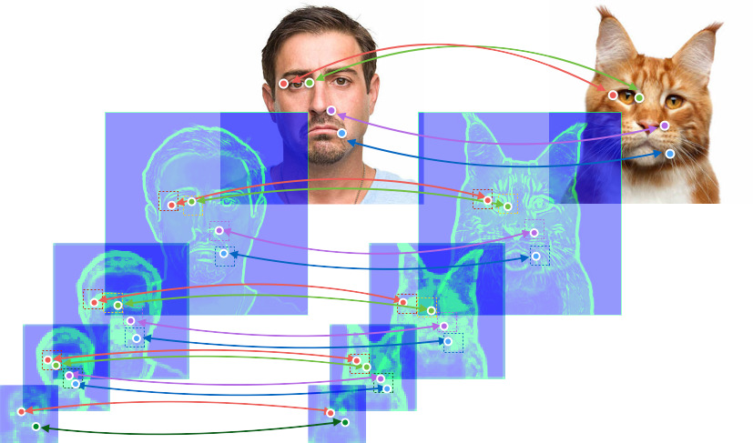
The spatial positions of the NBBs are refined as they are percolated through the hierarchy, in a coarse-to-fine fashion, by considering only the receptive field of each NBB neuron in the preceding layer of the CNN, until reaching the final positions in the original pair of input images (see the illustration in Figure 2.)
To enable the computation of the NBBs in a cross-domain setting, the features are first transformed to a common appearance, so that a simple patch correlation could be used effectively to measure point similarity. This is achieved using a simple style transfer technique that modifies the low-order statistics of the features in each pair of regions that we aim to match.
A variety of graphics applications, such as shape blending and image morphing, require cross-domain correspondences. However, these applications traditionally require manual interaction, leaving the semantic analysis task to the user. We demonstrate a number of such applications, evaluate the performance of our method, and compare it with other state-of-the-art methods. We show a number of fully automated image morphing sequences, created between objects from different semantic categories using our NBBs. In addition, the uniqueness of our approach is demonstrated via a new image hybridization application, where distinctive parts of two subjects are automatically combined into a hybrid creature, after aligning the two images based on our NBBs.
2. Related Work
2.1. Pairwise Keypoint Matching
In general, finding a sparse correspondence between two images involves two main steps: extracting individual key points (represented by descriptors), and performing metric-based matching.
There are various techniques to extract key points [Harris and Stephens, 1988], which are characterized by well-defined positions in the image space, local information content, and stability [Lindeberg, 2015]. However, in general, keypoint localization for generic object categories remains a challenging task. Most of the existing works on part localization or keypoint prediction focus on either facial landmark localization [Belhumeur et al., 2013; Kowalski et al., 2017] or human pose estimation [Gkioxari et al., 2014].
In order to identify the extracted points, a local descriptor is generated for each. Local invariant features such as SIFT [Lowe, 2004], SURF [Bay et al., 2006] and Daisy [Tola et al., 2010], has brought significant progress to a wide range of matching-based applications. These features are robust to typical appearance variations (e.g., illumination, blur) and a wide range of 2D transformations. However, these methods are unable to cope with major dissimilarities between the compared objects, such as strong color and shape differences.
More recently, various CNN-based descriptors were offered to replace traditional gradient based ones [Fischer et al., 2014]. Some of the descriptors are used for view-point invariance matching [Simonyan et al., 2014], others for discriminant patch representations [Simo-Serra et al., 2015]. Kim et al. [2017] offer a descriptor which is based on local self-similarity to robustly match points among different instances within the same object class.
Ufer et al. [2017] suggest a framework for sparse matching by extracting keypoints based on neuron activation, aiming at intra-class cases. However, the fact that the neurons are extracted from one specific layer together with imposed geometric constraints, limits their approach to mainly deal with same class cases, rather than two objects that exhibit a higher level of semantic similarity.
Following the keypoint extraction step, given two sets of descriptors, the matching process is usually performed using nearest neighbor matching, followed by an optional geometric verification. The one-directional matching obtained using the nearest neighbor field can be narrowed down by considering only mutual nearest neighbors. This method was previously leveraged for tasks such as image matching [Li et al., 2015], classification of images, etc., and extended to the Best-Buddies similarity concept, which measures similarity between patches [Dekel et al., 2015; Talmi et al., 2017] for the purpose of template matching.
We are not aware of any previous works which aim directly at finding sparse correspondence between two objects belonging to different semantic categories, as we do here.
2.2. Dense Correspondence
Normally, sparse matched keypoints constitute a basis for dense correspondence, which is a fundamental tool in applications such as stereo matching, and image registration. For the same scene scenario, a basic densification can be done by assuming a geometric model (affine, homography) that transforms between the two images. However, when the scenes are different, a simple geometric model cannot be assumed.
First steps towards semantic dense correspondence were made by Liu et al. [2011] with the development of SIFT flow. In their method, a displacement field is obtained by solving a discrete optimization problem in a hierarchical scheme, based on densely sampled SIFT features. Following SIFT flow, a number of other flow-based methods were suggested, e.g., Deep flow [Weinzaepfel et al., 2013] and Daisy flow [Yang et al., 2014], which perform matching of visually different scenes, and [Zhou et al., 2015] which proposes a net of correspondences between multiple same-class images, based on cycle-consistent connections. In parallel to the flow methods that assume smoothness of the flow field, the PatchMatch family [Barnes et al., 2009; Barnes et al., 2010] relaxes the rigidity assumption, yielding a dense patch-based nearest-neighbor field (NNF) instead. NRDC [HaCohen et al., 2011] extends generalized PatchMatch to cope with significant geometric and photometric variations of the same content.
In addition, CNN-based features (outputs of a certain convolution layer [Long et al., 2014], object proposals [Ham et al., 2016], etc.) have been employed with flow algorithms, and have shown potential to align intra-class objects better than handcrafted features. Zhou et al. [2016] suggested an end-to-end trained network that requires additional data in the form of synthetic rendered 3D models for formulating a cycle constraint between images. Choy et al. [2016] offered a unified system that learns correspondences based on annotated examples. However, this method is fully supervised, and in the case of cross-domain pairs it may be difficult to avoid ambiguities in the annotations. Liao et al. [2017], combine a coarse-to-fine deep feature pyramid with PatchMatch to compute a semantically-meaningful dense correspondence for transferring visual attributes between images. The images may differ in appearance, but must have perceptually similar semantic structure (same type of scene containing objects of similar classes). The above requirement, along with the goal of computing a dense mapping, makes their approach not well suited for our cross-domain scenario.
2.3. Image Morphing and Hybridization
Image morphing is a widely used effect [Wolberg, 1998], which typically requires a set of correspondences to define a warp field between the two images. With images of objects of the same class, such as two human faces, the necessary correspondences can be determined automatically in some cases, e.g., [Bichsel, 1996]. Morphing between images depicting objects from different classes requires user intervention to provide pairs of corresponding features, or explicit specification of a warp field [Liao et al., 2014]. Shechtman et al. [2010] applied patch-based texture synthesis to achieve interesting morph-like effect in a fully automated way, although this method is automatic it does not involves geometry warps, which make it hard to compare to the classic morph effect. We are not aware of any general, fully automated method, which is able to provide the correspondences necessary for image morphing between different objects that may even belong to different semantic classes. Our method enables automated image morphing which is not limited to perform in a specific domain.
Differing from image morphing, image hybridization refers to the process of assembling an image from different components from several source images. Hybridization can be performed by seamlessly fusing together parts from different images [Pérez et al., 2003; Huang et al., 2013]. Some hybridization methods are domain specific, e.g., [Bitouk et al., 2008] and [Korshunova et al., 2016]. Hybrid images may also be assembled from different spectral components, such that the image appears to change as the viewing distance changes [Oliva et al., 2006]. In this work we explore automatic as well as interactive cross-domain image hybridization.
3. Cross Domain Deep Correspondence
(a)

(b)
Given two images whose main regions of interest contain semantically related parts, or geometrically similar patterns, our goal is to find a set of pairwise correspondences. Furthermore, we strive to find correspondences for points positioned at semantically or geometrically meaningful locations.
Due to the differences in the shape and/or appearance of the objects, our approach is to exploit high-level information. Such information is encoded by the deep feature maps extracted by CNNs pretrained for the classification task. We represent these feature maps as a pyramid, whose top level contains the feature maps extracted by the last convolution layer, and the bottom level consists of the maps from the shallowest layer of the CNN (Section 3.1).
Our key idea is to propagate pairs of matching neurons from the top pyramid levels to the bottom ones, while narrowing down the search area at each step (see Figure 2), and focusing only on meaningful corresponding neurons at each level. Furthermore, in order to compensate for differences in appearance, which might be considerable in the cross-domain case, we first transform pairs of corresponding regions to a common local appearance, and only then perform a search for matching neurons. This approach is particularly necessary for finding correct matches within shallow feature maps, which are more strongly correlated with the appearance of the original image than those at deeper layers.
Note that we do not assume that deep features are invariant across domains. Rather, we only assume that corresponding features would be more similar to each other than to others in a small surrounding window. For example, we expect the features activated by an airplane wing to be more (mutually) similar to those activated by the wing of a goose than to those activated by other nearby parts. Thus, we define the corresponding neurons using the notion of meaningful Neural Best Buddies pairs (NBBs). Two neurons are considered best-buddies if they are mutual nearest neighbors, meaning that each neuron is the nearest neighbor of the other, among all the neurons in its set. Rather than keeping all of the NBB pairs, however, we only retain pairs where both neurons are strongly activated.
Following the extraction of two deep feature pyramids, three main steps are performed at each pyramid level: First, we extract NBB candidates from corresponding regions (Section 3.2). Second, the NBBs are selected based on the magnitudes of their activations (Section 3.4). Third, we propagate the remaining matches into the next hierarchy level, using the receptive fields of the NBB neurons to define refinement search regions around the propagated locations. Each pair of corresponding regions is transformed to a common appearance, as described in Section 3.3. Given the full resulting set of corresponding pairs, we explain in Section 3.5, how to pick high quality, spatially scattered correspondences. The above stages of our algorithm are summarized in Algorithm 1.
3.1. Deep Features Pyramid
Below, we elaborate on our coarse-to-fine analysis through the feature map hierarchy of a pre-trained network. Given two input images and , they are first fed forward through the VGG-19 network [Simonyan and Zisserman, 2014], to yield a five-level feature map pyramid (), where each level has progressively coarser spatial resolution. Specifically, the -th level is set to the feature tensor produced by the relu_1 layer of VGG-19. We denote these feature tensors of images and by and , respectively. The feature tensors of the last level capture all the information that enables the subsequent fully connected layers to classify the image into one of the ImageNet categories [Russakovsky et al., 2015]. It has been shown that the deeper layers of a trained network represent larger regions in the original image, encoding higher-level semantic information, which can be used as a descriptor for semantic matching, while the shallower layers encode lower level features over smaller image regions, such as edges, corners, and other simple conjunctions [Zeiler and Fergus, 2013]. We thus exploit the information encoded by the different layers, in order to find and localize semantic correspondences between two objects from different classes, which may differ in overall shape or appearance, but share some semantic similarities.
3.2. Neural Best Buddies
One of the challenges of cross-domain correspondence is that there are parts in one image, or even in the main object of interest, which have no correspondence in the other image/object. In order to avoid matching these incompatible regions, we utilize the concept of Neural Best Buddies pairs (NBBs), which are percolated through the deep features hierarchy, starting from the coarsest level to the finer ones. Specifically, at each level, the NBBs are computed only within pairs of corresponding regions defined by the receptive fields of the most meaningful NBBs discovered in the previous (coarser) level in the hierarchy. Let be a set of pairs of corresponding regions in the -th layer, where and are subsets of the spatial domains of and , respectively. In the top level (), the set of corresponding regions is initialized to a single pair , representing the entire domain of and .
For each pair of regions, , we extract its NBBs. More formally, a pair of neurons, , is defined as NBB pair if they are mutual nearest neighbors:
| (1) |
where is the Nearest Neighbor of neuron in the set under a similarity metric function :
| (2) |
Next, we define our deep feature similarity metric, , to facilitate the matching in a cross-domain setting.


| (a) | (b) |
3.3. Common Local Appearance
Naive patch similarity, using a metric such as between deep features, is valid only in the top levels, since lower levels are more strongly affected by color and appearance, which may differ significantly for cross-domain instances. Thus, to compensate for appearance differences at lower levels, we use style transfer to transform the corresponding regions to a common appearance, as illustrated in Figure 3. We use the notation of and to define the denote the transformed features and .
The similarity metric between two neurons and , is defined as the normalized cross-correlation between the common appearance version of their surrounding deep feature patches:
| (3) |
where and are the indices of the neighboring neurons of and , respectively. denotes the norm throughout the paper. The neighborhood size is determined by the level: we use for the two top levels () and for ..
Transferring the appearance or style of one image to another while keeping the content of the latter has recently been an active research area [Gatys et al., 2015; Johnson et al., 2016]. Various style transfer techniques can be used for our task, as long as they are applied locally on corresponding regions. For instance, the mechanism of Deep Image Analogy [Liao et al., 2017], which performs a local style transfer can be used to transfer corresponding areas to their middle appearnce, instead of transfering the style of one image to the content of the other and vice versa. In addtion, the idea presented by Huang et al. [2017] can be adopted. In this work the authors argue that instance normalization performs a form of style transfer by normalizing feature statistics, namely, the style is mainly contained in the mean and the variance of deep features channels. This technique greatly simplifies the transfer process and yield plausible results. In our context, however, we do not apply it globally over the entire image, but merely in local regions, which further increases the accuracy of the appearance matching:
| (4) |
where
| (5) |
and
| (6) |
are the mean and standard deviation of the common appearance, and and are the spatial mean and standard deviation over the denoted region, for each of the channels. is defined similarly, using as the source feature. The local transfer to a common appearance is illustrated in Figure 3. The advantage of our common appearance metric is demonstrated in Figure 4: we compute the NBBs between low level features () of two corresponding regions, and extracted using the process described in Section 3.5. As can be seen, the standard cross-correlation in low levels, which is based on color and shape, yields wrong corresponding positions, while our similarity metric localizes the corresponding points better.
3.4. Meaningful Best Buddies
Denote by the candidate NNBs computed in the -th level. At each level, before moving to next one, we filter pairs of best buddies based on their activation values, keeping only pairs where both neurons have strong activation values. This means that the paired neurons are deemed more significant by the CNN, in the top levels, and indicate significant low-level elements (corners, edges, etc.), in the bottom levels.
In order to be able to compare between activations of neurons from different layers, we compute a normalized activation map for each layer , which assigns each neuron a value in the range :
| (7) |
where is the unnormalized activation of a neuron at position in layer . is defined similarly with respect to .
Figure 5 visualizes the sum of the normalized activation maps over all layers of an image, after upsampling each layer’s activation map to the full image resolution. It may be seen that the highly ranked neurons are located in places that are important for the classification of the lion (the face, mane, legs and tail) and geometrically well defined (edges and corners).
Using the normalized activation maps, we seek NBBs which have high activation values, and filter the original set to create:
| (8) |
where is an empirically determined activation threshold.

| (a) | (b) |
Given , we next refine the filtered NBBs, by generating the finer consecutive set of corresponding search regions, , defined by their receptive field in the adjacent layer. In practice, due to observation of Long et al. [2014], which showed that similar features tend to respond to similar colors in the centers of their receptive fields, the search area in the finer layer is selected to be half of the receptive field. Then, we perform the search in each pair of corresponding search windows to extract
| (9) |
where
| (10) |
for a receptive field radius and central coordinates , as illustrated in Figure 2 (b). In our case, is equal to for and for .
We repeat this process for the levels. The final set of correspondences, , between the pixels of the two images , is set to the output of the last activation based filtering, . Note that the lowest layer, , has the same spatial resolution as the original image. The entire process is summarized in Algorithm 1.
3.5. Ranking and Spatial Distribution
The algorithm as described above produces a (non-fixed) number of NBB pairs. The corresponding pairs connect points of various quality and reliability, which are not necessarily well distributed across the regions of interest in each image. To rectify this situation, we refine the selection as described below.
We define the rank of a pair as the accumulated activation values of and through the levels of the feature hierarchy:
| (11) |
where and are the positions in the -th level that eventually led to the selection of and . The top pairs are unlikely to be well distributed across the images, since most of the highly ranked pairs lay around the same areas, e.g., eyes and mouth in the case of a face. To extract highly-ranked and well distributed pairs, we first partition our set of correspondences , into spatial clusters using the k-means algorithm. Next, in each cluster we select the pair with the highest rank. The effect of this process is demonstrated in Figure 6.
The coarse-to-fine selection of our algorithm is demonstrated in Figure 1 for , highly ranked, spatially scattered points. Each endpoint is annotated with circles that represent the receptive fields of its root points, at layers and , over the original image pixels.


4. Evaluation
In this section we evaluate the quality of our approach. It should be noted up front that we know of no other techniques that explicitly aim at cross-domain correspondence. This also implies that there are no established benchmarks for cross-domain correspondence. We clarify that a cross-domain pair, in this context, means that the images belong to different semantic categories in the ImageNet hierarchy [Russakovsky et al., 2015].
Thus, we evaluate our method using several different strategies: (i) we visually compare our NBB-based key point selection with other sparse matching techniques, (ii) we compare our correspondence to state-of-the-art dense correspondence methods, (iii) we perform a user study and compare the wisdom of the crowd statistics to our results, and finally, (iv) we test our method on pairs of objects with different scales, poses and view points to evaluate its robustness to various geometric deformations.
For every part in this section, many additional examples and results may be found in the supplementary material.
| Source | SIFT Flow [2011] | Proposal Flow[2016] | FCSS [2017] | Deep Analogy [2017] | Ours |
|---|---|---|---|---|---|
 |
 |
 |
 |
 |
 |
 |
 |
 |
 |
 |
 |
 |
 |
 |
 |
 |
 |
4.1. Pairwise Key-Point Localization
We first visually compare our method to other methods that aim at finding pairs of sparse corresponding key-points. Normally, these algorithms first extract points which constitute meaningful candidates for matching in every individual image, then search for their corresponding counterparts in the other image. Due to the fact that these methods were not explicitly designed to find cross-domain correspondence, we perform only a qualitative comparison, and use image pairs of progressive levels of difficulty: same object, intra-class, and cross-domain.
We compare our method with gradient-based descriptors and a technique based on deep features. Specifically, we use SIFT [Lowe, 2004] and SURF [Bay et al., 2006], by finding the strongest 10 matches using a threshold. In addition, we compare our method with Deep Semantic Feature Matching [Ufer and Ommer, 2017], a recent method, which first converts an image space pyramid to a deep features pyramid by transferring each level in the image pyramid to a specific deep layer (conv_4 of AlexNet [Krizhevsky et al., 2012]). The key points are selected based on the activation and entropy of the features, and the matching is done by minimizing an energy function that considers appearance and geometry.
The results are shown in Figure 7. For the gradient-based descriptors, the matches are marked by circles of corresponding color. In addition, we indicate with red crosses strong key-points that have no matches. As expected, it can be seen that the handcrafted descriptors cannot handle differences in appearance, including intra-class cases. In addition, it may be seen that deep semantic feature matching [Ufer and Ommer, 2017], which uses in fact only one layer of deep features, is unable to handle large differences in appearance, which are typical for cross-domain cases. The combination of our coarse-to-fine reconstruction and the common appearance transfer enables our approach to identify well-localized semantic similar pairs. Note, in particular, the highly non-trivial matching pairs between the images of the shark and the clownfish, where the other methods fail completely.
4.2. Dense Correspondence
We compare our method to state-of-the-art dense correspondence methods. We separate our evaluation into two parts: cross-domain cases and intra-class pairs.
Cross-Domain
Dense correspondence methods are typically not designed to handle cross-domain image pairs. Nevertheless, they compute a dense correspondence field, and thus may be used, in principle, to map any point from one image to another. Figure 8 shows several tests designed to test whether by applying several state-of-the-art dense correspondence in this manner, it might be possible to map the key points detected in one image to reasonable matching location in the other. For these tests, we use several cross-domain image pairs. Each image pair contains objects from different semantic categories, which exhibit drastic differences in appearance, yet feature some semantically similar parts (wheels, eyes, etc.)
The methods used in this evaluation are: SIFT Flow [Liu et al., 2011], Proposal Flow [Ham et al., 2016], FCSS [Kim et al., 2017], and Deep Image Analogy [Liao et al., 2017]. FCSS is a self-similarity descriptor that is based on a deep network and aims to robustly match points among different instances within the same object class. Kim et al. [2017] use a standard flow-based technique to generate a dense correspondence field from this descriptor. Deep Image Analogy is designed for visual attribute transfer (combining the content of one image with the style of another). It performs the nearest neighbors search, based on PatchMatch [Barnes et al., 2009], and controlled by parameters which dictate the relative contributions of the content and style sources. Figure 8 shows the mapping predicted by these methods for the key points suggested by our approach, and compares them to our result (rightmost column). With the absence of a ground truth, the results may only be evaluated qualitatively. Apart from our method and Deep Image Analogy, it is apparent that differences in appearance prevent the other methods to find a reasonable corresponding location for many of the points. While points on wheels of the car and the motorcycle are matched reasonably, this is not the case for other points, such as the tiger’s teeth. Also note that many of the points are not mapped onto the foreground object, but rather onto the surrounding background. While Deep Image Analogy typically finds correspondences on the foreground object, it may be seen that some of the matches are erroneous or less precisely localized. We attribute these differences to its use of random search and reliance on parameters that should be fine tuned. This point will be further elaborated in the next section.
Intra-Class
In order to quantitatively evaluate our method, we further compare it against an annotated ground truth benchmark of intra-class objects. We use the Pascal 3D+ dataset [Xiang et al., 2014], which provides sparse corresponding sets for same class objects with different appearance. For each category, we exhaustively sample all image pairs from the validation set, and make a comparison between our method to SIFT Flow [Liu et al., 2011], Proposal Flow [Ham et al., 2016], FCSS [Kim et al., 2017], Deep Image Analogy [Liao et al., 2017] and 3D Cycle Consistency [Zhou et al., 2016]. Cycle consistency is a representative work that considers high-level semantic information for dense matching. Since this method assumes having a shared 3D model of the class, we found it appropriate to include it only in the intra-class comparison.
Correctness of correspondences is measured by the percentage of correct keypoint transfers (PCK). A transfer is considered correct if the predicted location falls within pixels from the ground-truth, where and are the height and width of the image. We compute the PCK over all the pairs in each category.
Since the benchmark consists of point pairs that may differ from the ones produced by our method, we first extend our sparse correspondence into a dense one. This is done by interpolating our correspondences with Moving Least Squares (MLS) [Schaefer et al., 2006] warping field, which is described in more detail in Section 5.1.
The quantitative comparisons between different methods, using PCK with , are shown in Table 1 and visual comparisons on representative pairs are shown in Figure 9. Our method and deep image analogy, obtain better performance than methods based on low-level features, e.g., SIFT Flow. In addition, our method performs better than cycle consistency (often by a significant margin), even though the features we use were not trained on the Pascal 3D+ dataset.
|
Source |
 |
 |
 |
|---|---|---|---|
|
SIFT Flow |
 |
 |
 |
|
Proposal Flow |
 |
 |
 |
|
FCSS |
 |
 |
 |
|
3D Cycle |
 |
 |
 |
|
Deep Analogy |
 |
 |
 |
|
Ours |
 |
 |
 |
|
Target |
 |
 |
 |
| aeroplane | bicycle | boat | bottle | bus | car | chair | table | motorbike | sofa | train | monitor | mean | |
|---|---|---|---|---|---|---|---|---|---|---|---|---|---|
| SIFT Flow | 10.3 | 10.9 | 3.4 | 23.5 | 13.0 | 13.4 | 8.2 | 5.2 | 9.1 | 15.3 | 13.6 | 22.1 | 12.3 |
| Proposal Flow | 14.3 | 9.7 | 12.4 | 38.6 | 9.1 | 14.2 | 21.4 | 15.3 | 10.7 | 23.9 | 6.5 | 25.1 | 16.7 |
| FCSS | 20.7 | 22.2 | 11.8 | 50.0 | 22.5 | 31.3 | 18.2 | 14.2 | 15 | 28.9 | 8.7 | 30 | 22.8 |
| 3D Cycle | 20.8 | 25.0 | 4.9 | 51.0 | 21.1 | 33.8 | 37.9 | 11.9 | 15.0 | 32.2 | 13.7 | 33.8 | 25.0 |
| Deep Image Analogy | 20.0 | 34.2 | 7.9 | 44.3 | 18.2 | 33.8 | 38.7 | 10.9 | 17.0 | 38.4 | 14.7 | 35.8 | 28.3 |
| Ours | 21.4 | 38.8 | 14.0 | 48.2 | 32.5 | 33.2 | 26.3 | 20.0 | 23.4 | 48.4 | 24.8 | 45.8 | 31.4 |
4.3. User evaluation
In the case of same-scene images or intra-class objects, it is pretty straightforward for humans to annotate semantically similar points. However, in case of cross-domain instances, the matches are more ambiguous, and there might be no obvious or unique pixel-to-pixel matches. To evaluate the matching obtained by NBB, we conducted a user study. Each of the 30 study participants was shown 5 image pairs, which were chosen randomly each time from a larger set of 13 cross-domain pairs. Each participant was presented with points in the first image, and was asked to indicate best corresponding points in the second image. The points were automatically extracted by our method, as described in Section 3.5.
In order to quantitatively evaluate our algorithm based on the collected user annotations, we measure how well our results, as well as those of other algorithms, are aligned with these annotations. Specifically, for each individual point, we define the similarity measurement between that point and the user annotations to be the value of the probability density function at the point, where the density function is a 2D Gaussian distribution, whose parameters are estimated using maximum likelihood. Thus, when there is a strong consensus among the users regarding the position of the corresponding point, any significant deviation will be assigned a low score, unlike the case where the variance between the different users is large. For each algorithm we averaged the score of all the points. The results are shown in Table 2.
For qualitative evaluation, three results are demonstrated in Figure 10. The first image in each pair (first row) is the one that was presented to the users with 5 points (dots of different color). On the second image in each pair (second row), we visualize the Gaussian distribution of the users’ responses using ellipses of corresponding color. We also performed k-means clustering of the responses for each color into four clusters, and show the centers of the clusters as colored dots. The corresponding points found by our approach are marked as stars on the same image.
Note that the corresponding points indicated by different users exhibit considerable variance, due to the semantic uncertainty of their true location. This is especially evident in Fig. 10(a), where both the structures of the sailboat and the yacht and the viewpoint differ greatly. Nevertheless, it can be seen that the matches produced by our approach are well aligned with the distribution of human annotations.

| (a) | (b) | (c) |
| SIFT | Proposal | FCSS | Deep Image | Ours | |
| Flow | Flow | Analogy | |||
| Score | 0.032 | 0.042 | 0.084 | 0.123 | 0.163 |
4.4. Robustness and Limitations
Pose and Scale
In order to test the robustness of our method to pose differences, we match the same cow image to four images of horses, each featuring a different pose. The results are shown in Figure 11. It may be seen that our method can cope quite well with these cross-domain objects, despite the different poses.
As for robustness to scale differences: although we utilize a hierarchy of features, our method searches for best-buddies only between features at the same level, which might be interpreted as sensitivity to scale. However, since the classification network is trained for scale invariance, this invariance is reflected in its deep features. For instance, Figure 6 demonstrates correct matches between the giraffe and the cow heads despite their different scale. A stress test demonstrating robustness to scale differences is included in the supplementary material.

Erroneous matches
We next show that the information which is encoded in the high-level features is not purely semantic and geometry might also influence similarity of deep patches. This might lead to erroneous semantic correspondence and missing matches. For example, Figure 12 demonstrates such a failure case where the round silhouette of the man’s bald head shares highly correlated features with the edges of the dog’s ears, leading to semantically incorrect corresponding pairs. In addition, due to the significant geometry differences, between their nose and mouth, the network is unable to localize shared points around these semantically similar areas, which is a challenging task even for a human. Figure 12 (b) shows the correlation between each cell in the layer of one image and its nearest neighbor in the other corresponding map. It can be seen that high correlation exists around the bald head and the dog’s ears, while the correlation around the nose and mouth is relatively low.

| (a) | (b) |
5. Applications
Having computed a sparse set of correspondences between a pair of cross domain images, it is possible to warp the two images, such that their matching content becomes aligned, as well as to define a dense correspondence field between the two images. This, in turn, enables a variety of graphics applications, some of which are discussed below.
We note that the warping operations are performed in the pixel domain. The deep features extracted by the VGG network are intentionally translation invariant; thus, applying non-translational transformations directly onto the deep feature maps could lead to distortions in the reconstructed image.
5.1. Cross-Domain Image Alignment
Given a sparse set of NBBs for a pair of cross-domain images, our goal is to define a continuous warping field that would align the NBB pairs, while distorting the rest of the image as little as possible. Rather than applying optical flow or Nearest-Neighbor Field methods, we employ the moving least squares (MLS) image deformation method [Schaefer et al., 2006] for this purpose. More specifically, given a set of matching pairs , we compute a set of midpoints . The two images are then aligned by warping each of them such that its set of matched points is aligned with .

(a)

(b)
5.2. Semantic Hybridization
A hybrid image is one formed by combining parts from two images of different subjects, such that both subjects contribute to the result. Admittedly, this is not a well defined task; the hybridization strategy can be dictated by an artist, who selects which segments or attributes should be selected from each image, which segments to blend, and how to combine the colors [Benning et al., 2017]. As discussed below, aligning cross-domain images can be instrumental in this process, but it also makes it possible to create some interesting image hybrids automatically.
Given two cross-domain images, we aim to include in the hybrid their most semantically important and distinctive parts. This is done by first aligning the two images, as described above, and then combining their deep feature maps in a coarse-to-fine fashion.
Specifically, given two aligned images and , the goal is to generate a binary mask that indicates which areas of each input image are considered to be more meaningful and discriminative, and thus should be included in the hybrid.
We begin by forming such a mask for the coarsest level () of the deep features pyramid, defined as described in Section 3.1. The two feature tensors corresponding to the two aligned images and are normalized, and a hybrid feature tensor is formed by taking the most strongly activated neuron at each spatial location:
| (12) |
The hybrid feature map is then propagated down the hierarchy. To obtain the map from , we first use feature inversion [Mahendran and Vedaldi, 2015], without regularization, to obtain an inverted feature map , which is then projected onto the space of hybrids of and . Specifically,
| (13) |
When reaching the pixel level (), we do not perform the projection above, and use the inverted feature map as the resulting image hybrid, since this produces slightly softer transitions across boundaries between regions from different images.
Figure 13(a) demonstrates the process described above, and the final hybrid shown in Figure 13(b), along with two additional examples. It can be seen that in each of the examples the unique, discriminative parts of the animal, were selected automatically, i.e., the comb of the rooster, the eagle’s beak, the deer’s antlers.
Our cross-domain alignment may also be used by an interactive tool that enables artists to effortlessly produce hybrid images.
 |
 |
 |
5.3. Automatic Cross-Domain Image Morphing
The process of image morphing is based on dense correspondence with well defined motion paths. Typically, the motion paths are first defined between sparse corresponding features and then interpolated into dense smooth trajectories. Based on these trajectories, the images are warped and blended, to produce an animation. Since in many cases, an effective morph requires a semantic understanding of the image content, creating this mapping usually involves significant user interaction, using tagged features such as points, lines, curves, or grids [Wolberg, 1998].
Below, we utilize our sparse NBBs to modify the semi-automated image morphing method of Liao et al. [2014] into a fully automated method for cross-domain images. Liao et al. generate a dense correspondence between two images by minimizing the following energy functional:
| (14) |
where the first term is the SSIM index [Wang et al., 2004], which is responsible to rank the distances between pairs of patches, the second is the thin-plate spline (TPS) smoothness term, while the last term ensures that the warping field follow the set of sparse correspondences. After finding a dense correspondence, pixel trajectories are defined using quadratic motion paths. We refer the reader to [Liao et al., 2014] for more details.
In the original method of Liao et al. [2014], the third term is provided by the user, by manual marking of corresponding points. This part is crucial for the success of the morph, especially in the case of cross-domain instances. In our implementation, these manual correspondences are replaced with our automatically determined NBBs. Figure 14 shows the resulting morph on three cross-domain examples. These results are fully automatic.
Comparison.
Our method enables alignment between similar parts of human and animal faces, as can be seen in various examples in the paper and in the supplementary material. Using the morphing application, we next compare our face alignment with two methods designed specifically for automatic extraction of facial landmarks. The first method is geometry based [Zhu et al., 2015] and the other is deep learning based [Kowalski et al., 2017]. Both methods consist of two steps: face region detection and landmark extraction. It should be noted that these methods are not intended for animal faces and, indeed, these methods fail in the face detection stage. After manually marking the animals’ face regions, the methods were able to extract some landmarks, which we used as corresponding points to replace our NBBs in the term of Eq. (14). We present the middle image of the resulting sequences in Figure 15.

(a)
(b)
(c)
6. Conclusions and future work
We have presented a technique for sparse correspondence between cross-domain images. The technique is based on computation of best buddies pairs between the deep feature maps of a pre-trained classification CNN. The performance of our method goes a step beyond state-of-the-art correspondence methods, allowing to establish correspondence between images that do not share common appearance, and their semantic point correspondences are not necessarily obvious by considering local geometry.
Our automatic correspondences are surprisingly very close to those made manually by humans. We attribute this to the following factors: (i) the analysis is based on a pre-trained network, whose features at the deeper layers exhibit different kinds of invariance and were trained for semantic classification; (ii) our hierarchical analysis focuses only on regions that were indicated to have high-level similarity; (iii) as we go down the hierarchy, we search for best buddies in rather small regions, which are easier to bring to a common ground, thereby facilitating local matching; and (iv) the search focuses only on highly active regions, avoiding spurious matches.
Encouraged by our results, we are considering a number of avenues to continue exploring the use of neural best buddies. One avenue is considering a set of images, and applying co-analysis and co-segmentation, where the best buddies are mutual across the set. Since the neural best buddies are located in regions that are active in classification, we believe that they can also facilitate in foreground extraction. Another research avenue is to further advance the hybrid application. We believe that the combination of sparse cross-domain correspondence together with a deep analysis of the activation maps, can lead to creation of coherent hybrids of different objects. Lastly, we would also like to consider developing neural best buddies over pre-trained networks, which were trained for tasks other than classification.
7. Acknowledgments
We thank the anonymous reviewers for their helpful comments. This work is supported by National 973 Program (No.2015CB352500) of China and the ISF-NSFC Joint Research Program (2217/15, 2472/17).
References
- Barnes et al. [2009] Connelly Barnes, Eli Shechtman, Adam Finkelstein, and Dan B Goldman. 2009. PatchMatch: A randomized correspondence algorithm for structural image editing. ACM Transactions on Graphics (TOG) 28, 3 (2009), Article no. 24.
- Barnes et al. [2010] Connelly Barnes, Eli Shechtman, Dan B Goldman, and Adam Finkelstein. 2010. The generalized patchmatch correspondence algorithm. In Proc. ECCV. Springer, 29–43.
- Bay et al. [2006] Herbert Bay, Tinne Tuytelaars, and Luc Van Gool. 2006. Surf: Speeded up robust features. Computer vision–ECCV 2006 (2006), 404–417.
- Belhumeur et al. [2013] Peter N Belhumeur, David W Jacobs, David J Kriegman, and Neeraj Kumar. 2013. Localizing parts of faces using a consensus of exemplars. IEEE Transactions on Pattern Analysis and Machine Intelligence 35, 12 (2013), 2930–2940.
- Benning et al. [2017] Martin Benning, Michael Möller, Raz Z Nossek, Martin Burger, Daniel Cremers, Guy Gilboa, and Carola-Bibiane Schönlieb. 2017. Nonlinear Spectral Image Fusion. In International Conference on Scale Space and Variational Methods in Computer Vision. Springer, 41–53.
- Bichsel [1996] Martin Bichsel. 1996. Automatic interpolation and recognition of face images by morphing. In Proc. Second International Conference on Automatic Face and Gesture Recognition. IEEE, 128–135.
- Bitouk et al. [2008] Dmitri Bitouk, Neeraj Kumar, Samreen Dhillon, Peter Belhumeur, and Shree K Nayar. 2008. Face swapping: automatically replacing faces in photographs. ACM Transactions on Graphics (TOG) 27, 3 (2008), 39.
- Choy et al. [2016] Christopher B Choy, JunYoung Gwak, Silvio Savarese, and Manmohan Chandraker. 2016. Universal correspondence network. In Advances in Neural Information Processing Systems. 2414–2422.
- Dekel et al. [2015] Tali Dekel, Shaul Oron, Michael Rubinstein, Shai Avidan, and William T Freeman. 2015. Best-buddies similarity for robust template matching. In Proc. CVPR. IEEE, 2021–2029.
- Fischer et al. [2014] Philipp Fischer, Alexey Dosovitskiy, and Thomas Brox. 2014. Descriptor matching with convolutional neural networks: a comparison to sift. arXiv preprint arXiv:1405.5769 (2014).
- Gatys et al. [2015] Leon A Gatys, Alexander S Ecker, and Matthias Bethge. 2015. A neural algorithm of artistic style. arXiv preprint arXiv:1508.06576 (2015).
- Gkioxari et al. [2014] Georgia Gkioxari, Bharath Hariharan, Ross Girshick, and Jitendra Malik. 2014. Using k-poselets for detecting people and localizing their keypoints. In Proceedings of the IEEE Conference on Computer Vision and Pattern Recognition. 3582–3589.
- HaCohen et al. [2011] Yoav HaCohen, Eli Shechtman, Dan B Goldman, and Dani Lischinski. 2011. Non-rigid dense correspondence with applications for image enhancement. ACM transactions on graphics (TOG) 30, 4 (2011), 70.
- Ham et al. [2016] Bumsub Ham, Minsu Cho, Cordelia Schmid, and Jean Ponce. 2016. Proposal flow. In Proc. CVPR. IEEE, 3475–3484.
- Harris and Stephens [1988] Chris Harris and Mike Stephens. 1988. A combined corner and edge detector.. In Proc. Alvey Vision Conference, Vol. 15. Manchester, UK, 10–5244.
- Huang et al. [2013] Hui Huang, Kangxue Yin, Minglun Gong, Dani Lischinski, Daniel Cohen-Or, Uri M Ascher, and Baoquan Chen. 2013. " Mind the gap": tele-registration for structure-driven image completion. ACM Trans. Graph. 32, 6 (2013), 174–1.
- Huang and Belongie [2017] Xun Huang and Serge Belongie. 2017. Arbitrary style transfer in real-time with adaptive instance normalization. arXiv preprint arXiv:1703.06868 (2017).
- Johnson et al. [2016] Justin Johnson, Alexandre Alahi, and Li Fei-Fei. 2016. Perceptual losses for real-time style transfer and super-resolution. In Proc. ECCV. Springer, 694–711.
- Kim et al. [2017] Seungryong Kim, Dongbo Min, Bumsub Ham, Sangryul Jeon, Stephen Lin, and Kwanghoon Sohn. 2017. FCSS: Fully convolutional self-similarity for dense semantic correspondence. arXiv preprint arXiv:1702.00926 (2017).
- Korshunova et al. [2016] Iryna Korshunova, Wenzhe Shi, Joni Dambre, and Lucas Theis. 2016. Fast face-swap using convolutional neural networks. arXiv preprint arXiv:1611.09577 (2016).
- Kowalski et al. [2017] Marek Kowalski, Jacek Naruniec, and Tomasz Trzcinski. 2017. Deep Alignment Network: A convolutional neural network for robust face alignment. arXiv preprint arXiv:1706.01789 (2017).
- Krizhevsky et al. [2012] Alex Krizhevsky, Ilya Sutskever, and Geoffrey E Hinton. 2012. Imagenet classification with deep convolutional neural networks. In Advances in neural information processing systems. 1097–1105.
- Li et al. [2015] Ting-ting Li, Bo Jiang, Zheng-zheng Tu, Bin Luo, and Jin Tang. 2015. Image matching using mutual k-nearest neighbor graph. In International Conference of Young Computer Scientists, Engineers and Educators. Springer, 276–283.
- Liao et al. [2014] Jing Liao, Rodolfo S Lima, Diego Nehab, Hugues Hoppe, Pedro V Sander, and Jinhui Yu. 2014. Automating image morphing using structural similarity on a halfway domain. ACM Transactions on Graphics (TOG) 33, 5 (2014), 168.
- Liao et al. [2017] Jing Liao, Yuan Yao, Lu Yuan, Gang Hua, and Sing Bing Kang. 2017. Visual Attribute Transfer Through Deep Image Analogy. ACM Trans. Graph. 36, 4, Article 120 (July 2017), 15 pages. https://doi.org/10.1145/3072959.3073683
- Lindeberg [2015] Tony Lindeberg. 2015. Image matching using generalized scale-space interest points. Journal of Mathematical Imaging and Vision 52, 1 (2015), 3–36.
- Liu et al. [2011] Ce Liu, Jenny Yuen, and Antonio Torralba. 2011. Sift flow: Dense correspondence across scenes and its applications. IEEE Transactions on Pattern Analysis and Machine Intelligence 33, 5 (2011), 978–994.
- Long et al. [2014] Jonathan L Long, Ning Zhang, and Trevor Darrell. 2014. Do convnets learn correspondence?. In Advances in Neural Information Processing Systems. 1601–1609.
- Lowe [2004] David G Lowe. 2004. Distinctive image features from scale-invariant keypoints. International Journal of Computer Vision 60, 2 (2004), 91–110.
- Mahendran and Vedaldi [2015] Aravindh Mahendran and Andrea Vedaldi. 2015. Understanding deep image representations by inverting them. In Proceedings of the IEEE conference on computer vision and pattern recognition. 5188–5196.
- Oliva et al. [2006] Aude Oliva, Antonio Torralba, and Philippe G Schyns. 2006. Hybrid images. In ACM Transactions on Graphics (TOG), Vol. 25. ACM, 527–532.
- Pérez et al. [2003] Patrick Pérez, Michel Gangnet, and Andrew Blake. 2003. Poisson image editing. In ACM Transactions on graphics (TOG), Vol. 22. ACM, 313–318.
- Russakovsky et al. [2015] Olga Russakovsky, Jia Deng, Hao Su, Jonathan Krause, Sanjeev Satheesh, Sean Ma, Zhiheng Huang, Andrej Karpathy, Aditya Khosla, Michael Bernstein, Alexander C. Berg, and Li Fei-Fei. 2015. ImageNet large scale visual recognition challenge. International Journal of Computer Vision 115, 3 (Dec 2015), 211–252.
- Schaefer et al. [2006] Scott Schaefer, Travis McPhail, and Joe Warren. 2006. Image deformation using moving least squares. ACM transactions on graphics (TOG) 25, 3 (2006), 533–540.
- Shechtman et al. [2010] Eli Shechtman, Alex Rav-Acha, Michal Irani, and Steve Seitz. 2010. Regenerative morphing. In Computer Vision and Pattern Recognition (CVPR), 2010 IEEE Conference on. IEEE, 615–622.
- Simo-Serra et al. [2015] Edgar Simo-Serra, Eduard Trulls, Luis Ferraz, Iasonas Kokkinos, Pascal Fua, and Francesc Moreno-Noguer. 2015. Discriminative learning of deep convolutional feature point descriptors. In Proc. ICCV. IEEE, 118–126.
- Simonyan et al. [2014] Karen Simonyan, Andrea Vedaldi, and Andrew Zisserman. 2014. Learning local feature descriptors using convex optimisation. IEEE Transactions on Pattern Analysis and Machine Intelligence 36, 8 (2014), 1573–1585.
- Simonyan and Zisserman [2014] Karen Simonyan and Andrew Zisserman. 2014. Very deep convolutional networks for large-scale image recognition. arXiv preprint arXiv:1409.1556 (2014).
- Talmi et al. [2017] Itamar Talmi, Roey Mechrez, and Lihi Zelnik-Manor. 2017. Template Matching with Deformable Diversity Similarity. In Proc. CVPR. IEEE.
- Tola et al. [2010] Engin Tola, Vincent Lepetit, and Pascal Fua. 2010. Daisy: An efficient dense descriptor applied to wide-baseline stereo. IEEE transactions on pattern analysis and machine intelligence 32, 5 (2010), 815–830.
- Ufer and Ommer [2017] Nikolai Ufer and Bjorn Ommer. 2017. Deep semantic feature matching. In Proc. CVPR. IEEE, 5929–5938.
- Wang et al. [2004] Zhou Wang, Alan C Bovik, Hamid R Sheikh, and Eero P Simoncelli. 2004. Image quality assessment: from error visibility to structural similarity. IEEE Transactions on Image Processing 13, 4 (2004), 600–612.
- Weinzaepfel et al. [2013] Philippe Weinzaepfel, Jerome Revaud, Zaid Harchaoui, and Cordelia Schmid. 2013. DeepFlow: Large displacement optical flow with deep matching. In Proc. ICCV. 1385–1392.
- Wolberg [1998] George Wolberg. 1998. Image morphing: a survey. The Visual Computer 14, 8 (1998), 360–372.
- Xiang et al. [2014] Yu Xiang, Roozbeh Mottaghi, and Silvio Savarese. 2014. Beyond pascal: A benchmark for 3d object detection in the wild. In Proc. WACV. IEEE, 75–82.
- Yang et al. [2014] Hongsheng Yang, Wen-Yan Lin, and Jiangbo Lu. 2014. Daisy filter flow: A generalized discrete approach to dense correspondences. In Proc. CVPR. 3406–3413.
- Yosinski et al. [2015] Jason Yosinski, Jeff Clune, Anh Mai Nguyen, Thomas J. Fuchs, and Hod Lipson. 2015. Understanding Neural Networks Through Deep Visualization. CoRR abs/1506.06579 (2015). arXiv:1506.06579 http://arxiv.org/abs/1506.06579
- Zeiler and Fergus [2013] Matthew D. Zeiler and Rob Fergus. 2013. Visualizing and Understanding Convolutional Networks. CoRR abs/1311.2901 (2013). arXiv:1311.2901 http://arxiv.org/abs/1311.2901
- Zhou et al. [2015] Tinghui Zhou, Yong Jae Lee, Stella X Yu, and Alyosha A Efros. 2015. Flowweb: Joint image set alignment by weaving consistent, pixel-wise correspondences. In Proceedings of the IEEE Conference on Computer Vision and Pattern Recognition. 1191–1200.
- Zhou et al. [2016] Tinghui Zhou, Philipp Krahenbuhl, Mathieu Aubry, Qixing Huang, and Alexei A Efros. 2016. Learning dense correspondence via 3d-guided cycle consistency. In Proc. CVPR. 117–126.
- Zhu et al. [2015] Shizhan Zhu, Cheng Li, Chen Change Loy, and Xiaoou Tang. 2015. Face alignment by coarse-to-fine shape searching. In Proceedings of the IEEE Conference on Computer Vision and Pattern Recognition. 4998–5006.