A data-driven method for the steady state of randomly perturbed dynamics

Consider an autonomous ordinary differential equation

(2.1)

$$x^{\prime}=f(x),\quad x\in\mathbb{R}^{n}\,.$$

We are particularly interested in situations when equation (2.1) generates non-trivial dynamics. For example, equation (2.1) may admit a strange attractor or have separation of time scales that leads to interesting dynamics like the folding singularity, mixed mode oscillations etc. [14, 10].

Now we consider the following dynamical system with random perturbations, i.e., a stochastic differential equation (SDE),

(2.2)

$$\mathrm{d}X_{t}=f(X_{t})\mathrm{d}t+\sigma(X_{t})\mathrm{d}W_{t}\,,$$

where $X_{t}\in\mathbb{R}^{n}$, $f:\mathbb{R}^{n}\rightarrow\mathbb{R}^{n}$ is a vector field, $\sigma:\mathbb{R}^{n}\rightarrow\mathbb{R}^{n\times n}$ is a matrix-valued function, and $\mathrm{d}W_{t}$ is the $n$-dimensional white noise. Throughout this paper, we assume that equation (2.2) admits a unique diffusion process solution $X_{t}$. (See (H) below for the full assumption.) Note that the existence and the uniqueness of $X_{t}$ follow from mild assumptions on $f$ and $\sigma$, e.g., Lipschitz continuity of $f$ and $\sigma$ [27, 18].

Since $X_{t}$ is a diffusion process, we denote the transition kernel of $X_{t}$ by $P^{t}(x,A)=\mathbb{P}[X_{t}\in A\,|\,X_{0}=x]$. A probability measure $\pi$ is said to be invariant if $\pi P^{t}=\pi$, where the left operator is defined as

$$\pi P^{t}(A)=\int_{\mathbb{R}^{n}}P^{t}(x,A)\pi(\mathrm{d}x)\,.$$

It is well known that the time evolution of the probability density function of $X_{t}$, denoted by $u_{t}$, is described by the Fokker-Planck equation

(2.3)

$$u_{t}=\mathcal{L}u=-\sum_{i=1}^{n}(f_{i}u)_{x_{i}}+\frac{1}{2}\sum_{i,j=1}^{n}(D_{i,j}u)_{x_{i}x_{j}}\,,\quad u(0,x)=u_{0}(x)\,,$$

where $D=\sigma^{T}\sigma$, $u_{0}(x)$ is the probability density function of $X_{0}$. A probability density function $u_{*}(x)$ is said to be an invariant probability density function if $\mathcal{L}u_{*}=0$. It is easy to see that an invariant probability density function defines an invariant probability measure $\pi$ of $X_{t}$, and $u_{*}(x)$ is the probability density function of $\pi$.

The existence of an invariant probability measure is guaranteed if $X_{t}$ is defined on a compact manifold without boundary [34]. When $X_{t}$ is defined on unbounded domain, such existence needs some “dissipation” conditions [4, 16, 19]. The uniqueness of $\pi$ usually follows if $D$ is non-degenerate (everywhere positive definite). The convergence to the invariant probability measure is another tricky issue. To make $P^{t}(x,\cdot)\rightarrow\pi$ as $t\rightarrow\infty$, one needs stronger “dissipation” conditions and some minorization-type conditions [25, 15, 19]. Since the theme of this paper is to introduce a numerical algorithm, we have the following assumption on $X_{t}$, $P^{t}(x,\cdot)$, and $\pi$ throughout the paper.

(H) Equation (2.2) admits a unique diffusion process $X_{t}$. The diffusion process $X_{t}$ has a unique invariant probability measure $\pi$ that is absolutely continuous with respect to the Lebesgue measure. The probability density function of $\pi$ uniquely solves the stationary Fokker-Planck equation. In addition, $P^{t}(x,\cdot)\rightarrow\pi$ as $t\rightarrow\infty$ for every $x\in\mathbb{R}^{n}$.

There are two different approaches for computing $u_{*}$. One can either solve the Fokker-Planck equation (2.3) up to a sufficiently large $t$, or solve the stationary Fokker-Planck equation directly. The biggest problem of the numerical PDE approach is the boundary condition. For the sake of simplicity, we illustrate the problem by using the finite difference scheme. The case of the finite element scheme is analogous.

Without loss of generality, we solve the Fokker-Planck equation numerically on a 2D domain $[-L,L]^{2}$. Let the spatial and time step sizes be $r=2L/N$ and $h$, respectively. Let $\mathbf{u}^{m}=\{u^{m}_{i,j}\}_{i,j=0}^{N}$ be the discretized solution at time step $m$. Entry $u^{m}_{i,j}$ is a numerical approximation of $u(mh,ri-L,rj-L)$. We need boundary conditions to update the solution to $\mathbf{u}^{m+1}$. The usual approach is to let the domain cover the global attractor of the ODE (2.1) with sufficient margin. Then we assume zero boundary conditions $u^{m}_{0,j}=u^{m}_{N,j}=u^{m}_{i,0}=u^{m}_{i,N}=0$ and compute $\mathbf{u}^{m+1}$ by using either implicit Euler scheme or Crank-Nickson scheme. Since the probability of $X_{t}\notin[-L,L]^{2}$ is nonzero, $\mathbf{u}^{m}$ needs to be renormalized after each update such that

$$\sum_{i,j=0}^{N}u^{m}_{i,j}=\frac{1}{r^{2}}\,.$$

When $\|\mathbf{u}^{m}-\mathbf{u}^{m-1}\|$ is smaller than the error tolerance $\epsilon$ for some $m=M$, the update is stopped. Now $\mathbf{u}^{M}$ numerically solves the steady state Fokker-Planck equation. In order to make the numerical solution reliable, the domain has to be sufficiently large such that $\mathbb{P}[X_{t}\notin[-L,L]^{2}]\ll 1$ for $t\in[0,Mh]$ and $1-\pi([-L,L]^{2})\ll 1$.

Another approach is to solve the steady state Fokker-Planck equation directly. Assume the same 2D domain as before. In order to discretize $\mathcal{L}u_{*}$, the boundary value of $u_{*}$ on $\partial[-L,L]^{2}$ is necessary. The usual practice is to make $L$ large enough so that $[-L,L]^{2}$ covers the global attractor of equation (2.1) with sufficient margin. Then we can assume a zero boundary condition because of the Freidlin-Wentzell theory [11]. This will generate a linear system

$$A\mathbf{u}=\mathbf{0}\,,$$

where $A$ is an $n\times n$ nonsingular matrix. To avoid the trivial solution, one also needs the constraint

$$\mathbf{1}^{T}\mathbf{u}=r^{-2}\,.$$

This gives an overdetermined linear system

(2.4)		$\displaystyle A\mathbf{u}$	$\displaystyle=$	$\displaystyle\mathbf{0}$
	$\displaystyle\mathbf{1}^{T}\mathbf{u}$	$\displaystyle=$	$\displaystyle r^{-2}\,.$

Let

$$\hat{A}=\begin{bmatrix}A\\ \mathbf{1}^{T}\end{bmatrix}\quad,\quad\mathbf{b}=\begin{bmatrix}\mathbf{0}\\ r^{-2}\end{bmatrix}\,.$$

We can find the least squares solution $\hat{\mathbf{u}}$ that solves the optimization problem

$$\min\|\hat{A}\hat{\mathbf{u}}-\mathbf{b}\|_{2}\,.$$

The least squares solution $\hat{\mathbf{u}}$ numerically solves the steady state Fokker-Planck equation.

The numerical PDE approach works reasonably well for 1D and 2D problems. However, in higher dimension this approach becomes not practical. In particular, the domain has to be sufficiently large to cover the global attractor of equation (2.1) with enough margin. This imposes great difficulty to many practical problems. For example, if equation (2.1) is a Lorenz system, then we need a grid in a $50\times 50\times 50$ box to cover the attractor. (See section 4.3 for more discussion about the Lorenz system.)

An alternative approach is to use Monte Carlo simulation. One can collect samples of $X_{t}$ over a long trajectory in any dimension, although the accuracy of the Monte Carlo simulation suffers greatly from the curse-of-dimensionality. Let $h\ll 1$ be the step size. Let $X_{n}:=X_{nh}$ be the numerical time-$h$ sample chain produced by certain numerical method (Euler, Milstein, Runge-Kutta .etc) [20]. Under certain conditions, $X_{n}$ admits an invariant probability measure $\pi_{h}$ that converges to $\pi$ as $h\rightarrow 0$ [24, 23]. In addition, $X_{n}$ is a Markov chain. Let $\xi:\mathbb{R}^{n}\rightarrow\mathbb{R}$ be an observable on $\mathbb{R}^{n}$ and $\mathbf{N}$ be the number of samples. By the law of large numbers of Markov chains [25], we have

$$\frac{1}{\mathbf{N}}\sum_{n=1}^{\mathbf{N}}\xi(X_{n})\rightarrow\pi(\xi)\quad a.s.\,.$$

Therefore, we can use Monte Carlo simulation to compute the probability density function of $\pi$. For the sake of simplicity we consider grid points $\mathbf{u}=\{u_{i,j}\}_{i,j=0}^{N}$ in a 2D domain $[-L,L]^{2}$, such that $u_{i,j}$ is the numerical approximation of $u_{*}(ir-L,jr-L)$. Let $O_{i,j}=[ir-L-r/2,ir-L+r/2]\times[jr-L-r/2,jr-L+r/2]$. Then the Monte Carlo simulation gives

$$u_{i,j}=\frac{1}{\mathbf{N}r^{2}}\sum_{n=1}^{N}\mathbf{1}_{O_{i,j}}(X_{n})$$

for some sufficiently large $\mathbf{N}$. In practice, we construct $(N+1)^{2}$ boxes $O_{i,j}$ and simulate $X_{n}$ over a long time period. After the simulation, $u_{i,j}$ is obtained by counting sample points of $X_{n}$ falling into $O_{i,j}$.

It is easy to see that the Monte Carlo simulation approach has a significant disadvantage on the accuracy because it is difficult to collect enough sample points in each $O_{i,j}$. Without loss of generality, we assume

$$\sum_{n=1}^{\mathbf{N}}\mathbf{1}_{O_{i,j}}(X_{n})=O(r^{2}\mathbf{N})\,.$$

If we treat $\mathbf{1}_{O_{i,j}}(X_{n})$ as i.i.d Bernoulli random variables, some calculation shows that the standard deviation of $u_{i,j}$ is $O(r^{-1}\mathbf{N}^{-1/2})$. Hence $\mathbf{N}$ has to be very large to control the standard deviation. For example, $\mathbf{N}$ needs to be $O(r^{-5})$ to reduce the standard deviation to $O(r^{2})$. The accuracy problem will be much worse in higher dimensions. In practice, the solution obtained from the Monte Carlo simulation usually looks very “noisy”.

Despite of its accuracy problem, the Monte Carlo simulation has more flexibility because of the following reasons. (1) In the Monte Carlo simulation, the domain $[-L,L]^{2}$ does not have to cover the global attractor of (2.1). (2) The curse of dimensionality is slightly alleviated if equation (2.1) has a lower dimensional global attractor. Because the invariant probability measure $\pi$ concentrates on the vicinity of the global attractor of equation (2.1). (3) Parallel computing is much easier for Monte Carlo simulations. (4) Some high dimensional sampling technique can be applied to improve the Monte Carlo simulation for a large class of dynamical systems.

The first example is the gradient flow with respect to a double-well potential. Consider the potential function

$$U=\frac{1}{2}x^{4}-x^{2}$$

and the stochastic differential equation

$$\mathrm{d}X_{t}=-U^{\prime}(X_{t})\mathrm{d}t+\sigma\mathrm{d}W_{t}$$

for $\sigma=0.6$. The probability density function of this system is

$$u_{*}(x)=\frac{1}{K}e^{-2U(x)/\sigma^{2}}\,,$$

where $K$ is a normalizer.

In this example, we demonstrate our method by solving for $u_{*}(x)$ on the interval of $[0,2]$. Note that this system has two equilibria at $\pm 1$. Equilibrium $x=-1$ is not covered by the numerical domain $[0,2]$. In particular, we have $u_{*}(0)=0.1062$ so the zero boundary condition does not apply to this problem. We also show the accuracy and computational time of the hybrid method in this example.

Let $X_{n}$ be the discrete-time Markov chain given by the Euler–Maruyama method with a fixed time step size $\mathrm{d}t=0.001$. The Monte Carlo simulation is done by simulating $X_{n}$ up to time $T=\mathbf{N}h$. The numerical solution from the optimization problem, the exact probability density function $u_{*}(x)$, and the approximate density function from Monte Carlo simulation are compared in Figure 1. We can see that the Monte Carlo simulation itself only produces a solution with low accuracy, unless one can collect a huge amount of samples. In fact, when $h=0.005$, $T$ needs to be at least $10^{5}$ to remove the sawtooth in the solution (the orange plot in Figure 1). The rough solution generated by the Monte Carlo simulation is smoothed and corrected by the linear constraint (the red plot in Figure 1).

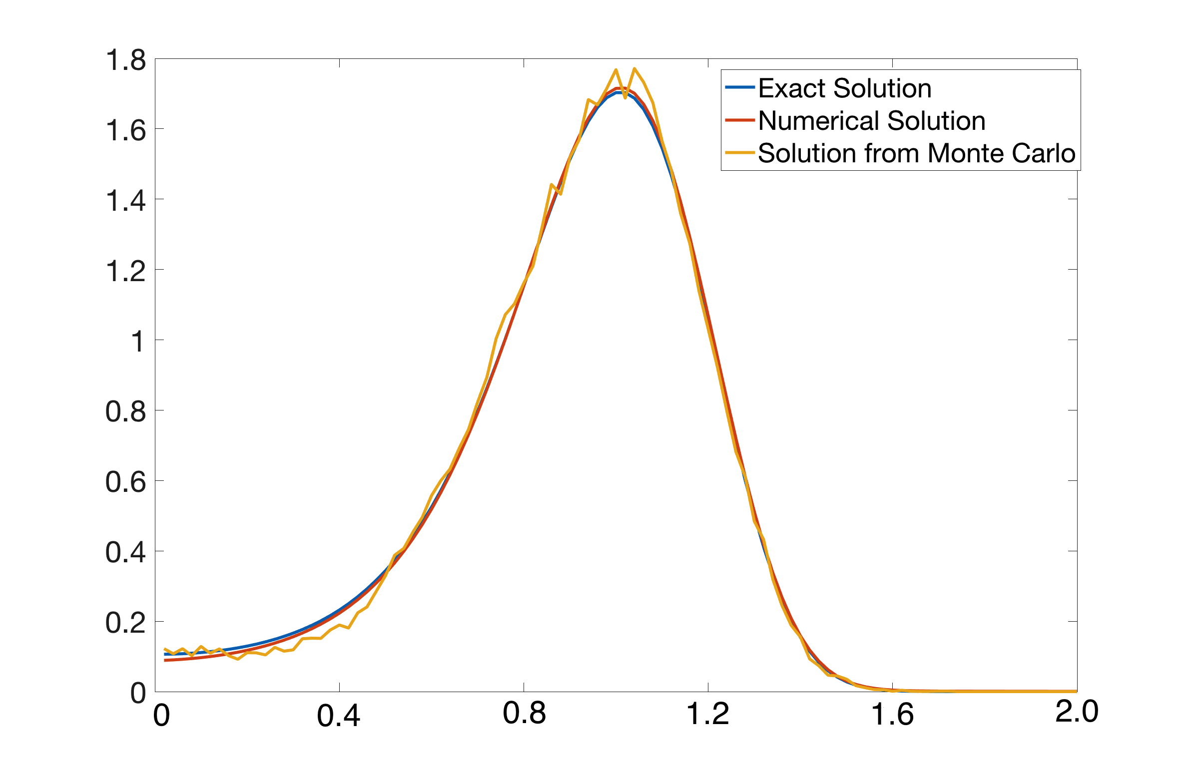
The following table compares $L^{2}$ errors with varying time span $T$ and grid size $h$. Each entry is the average $L^{2}$ error of $5$ trials. We can see that despite some randomness caused by the Monte Carlo simulation, the error drops with smaller grid size and larger sample size for the Monte Carlo simulation. Note that the invariant probability measure of $X_{n}$ is only an $O(\mathrm{d}t)=1.0\times 10^{-3}$ approximation of that of $X_{t}$. Hence it does not make sense to test the accuracy with more samples or smaller grid size unless one makes the time step even smaller. In this small-scale 1D problem, the classical numerical PDE solver is more accurate, mainly because the invariant probability measure of $X_{n}$ is only a first order approximation of that of $X_{t}$. But overall the accuracy is satisfactory given the performance of the algorithm.

It remains to comment on the computation time. We choose smaller grid sizes $h=2\times 10^{-4}$, $1\times 10^{-4}$, and $5\times 10^{-5}$ to highlight the difference between different approaches. The time span of Monte Carlo simulation is chosen to be $T=4000$. In order to apply the numerical PDE approach directly, one needs to enlarge the domain to $[-2,2]$ to apply the zero boundary condition. The direct Monte Carlo simulation is too slow to be interesting if one wants to achieve the same accuracy. Hence we only compare the numerical PDE approach and the hybrid method in the following table. The computation time for the hybrid method is further broken down in to the Monte Carlo simulation phase (Phase 1) and the optimization phase (Phase 2). The numerical PDE approach uses the MATLAB solver mldivide (the backslash solver). The Monte Carlo simulation is written in C++. The optimization problem equation (3.1) is solved by the MATLAB solver lsqminnorm.

From Table 2, we can find that solving the optimization problem (3.1) is actually much faster than solving the least squares problem (2.4). This is because the numerical PDE approach has to cover both equilibria with considerable margin in order to apply the zero boundary condition. In addition, solving the overdetermined least squares problem in equation (2.4) takes more time for the MATLAB solver we use. In this problem, the Monte Carlo simulation is the bottleneck of the hybrid method. In higher dimensional problems, such as the Lorenz oscillator in Section 4.3, solving the optimization problem (3.1) usually takes much more time than the Monte Carlo simulation. And the classical numerical PDE approach becomes not practical any more, because the domain still has to cover the entire attractor in order to apply the zero boundary condition.

The second example is a Van der Pol oscillator, which has been intensively used in both physics and mathematical biology [13, 17]. In this subsection, we use our method to demonstrate an interesting phenomenon related to the canard solution.

Consider an oscillator

(4.1)		$\displaystyle\dot{x}$	$\displaystyle=$	$\displaystyle\frac{1}{\epsilon}(y-\frac{1}{3}x^{3}+x)$
	$\displaystyle\dot{y}$	$\displaystyle=$	$\displaystyle a-x\,,$

where $\epsilon=0.1$ is the time scale separation parameter, and $a$ is a control parameter. This system is a prototypical example for the canard explosion. A “canard” is a solution that the system can pass a bifurcation point of the critical manifold and follow the repelling part of the slow manifold for some amount of time [3]. Usually a canard solution only exists for a very small range of parameters.

We consider the random perturbation of system (4.1)

(4.2)		$\displaystyle\mathrm{d}X_{t}$	$\displaystyle=$	$\displaystyle\frac{1}{\epsilon}(Y_{t}-\frac{1}{3}X_{t}^{3}+X_{t})\mathrm{d}t+\sigma\mathrm{d}W^{1}_{t}$
	$\displaystyle\mathrm{d}Y_{t}$	$\displaystyle=$	$\displaystyle(a-X_{t})\mathrm{d}t+\sigma\mathrm{d}W^{2}_{t}\,,$

where $W^{1}_{t}$ and $W^{2}_{t}$ are two independent Wiener processes. The parameter $a$ is chosen to be $0.9964$, at which the deterministic system has already passed the canard bifurcation and is attracted to a smaller limit cycle (blue curve in Figure 2). We use our hybrid method to compute the density function $u_{*}(x)$ of the invariant probability measure of system (4.2). Our numerical result shows that this transition through a canard solution is essentially destroyed by a small random perturbation. Although the deterministic system admits a smaller limit cycle, the steady state probability density function $u_{*}(x)$ still concentrates on the large limit cycle corresponding to the relaxation oscillations (the black curve in Figure 2). When the strength of noise increases, the support of $u_{*}(x)$ not only becomes “wider”, but also has significant deformation. When the noise is large ($\sigma=1.0$), some probability density moves to the slow manifold that does not belong to any limit cycle of the deterministic system and forms two “tails”. With the hybrid method introduced in this paper, we can get a high resolution local solution about the lower left “tail” with much higher precision (Panel 6 of Figure 3).

The hybrid method demonstrates its full strength in 3D systems. In this subsection, we compute numerical invariant probability density functions of two randomly perturbed chaotic systems: the Lorenz oscillator and the Rössler attractor. Both of them are typical chaotic oscillators that play a significant role in the study of nonlinear physics and dynamical systems [30, 12, 1, 22].

For the Lorenz system, we mean

(4.3)		$\displaystyle\dot{x}$	$\displaystyle=$	$\displaystyle a(y-x)$
	$\displaystyle\dot{y}$	$\displaystyle=$	$\displaystyle x(b-z)-y$
	$\displaystyle\dot{z}$	$\displaystyle=$	$\displaystyle xy-cz$

with typical parameters $a=10$, $b=28$, and $c=8/3$. It is well known that system (4.3) has a butterfly-shape strange attractor. The Rössler attractor is a chaotic oscillator that has the similar mechanism as the Lorenz oscillator. We have

(4.4)		$\displaystyle\dot{x}$	$\displaystyle=$	$\displaystyle-y-z$
	$\displaystyle\dot{y}$	$\displaystyle=$	$\displaystyle x+ay$
	$\displaystyle\dot{z}$	$\displaystyle=$	$\displaystyle b+z(x-c)\,.$

Again, we use typical parameters $a=0.2,b=0.2$, and $c=5.7$.

We are interested in invariant probability density functions of random perturbations of system (4.3) and system (4.4). In both systems, a perturbation term $\sigma\mathrm{d}\mathbf{W}_{t}$ is added to the deterministic part, where $\sigma>0$ is the strength of noise, and $\mathbf{W}_{t}$ is the standard Wiener process in $\mathbb{R}^{3}$. Needless to say, it is extremely difficult to solve a steady state Fokker-Planck equation in 3D on a large domain. Take the Lorenz oscillator as an example. If the numerical domain has to cover the attractor, we will solve a 3D equation on a cube $[-25,25]\times[-25,25]\times[0,50]$. When the grid size is $0.05$, the resultant numerical solution will have $10^{9}$ grid points. Solving such a large linear system is very computationally expensive.

The hybrid method provides an approach to solve a 3D steady state Fokker-Planck equation locally with high resolution and low cost. If the global solution is still necessary, one can numerically solve many local solutions and “glue” them together. In Figure 4, we choose a small box on the attractor as the domain (the red rectangle). The attractor is projected to the XY-plane for the purpose of demonstration. Note that the Lorenz oscillator is rotated by a rotation matrix for the purpose of easier demonstration and mesh generation. The heights of both domains are $1.0$. Then we use our hybrid method to compute the invariant probability density function. The strength of noise is chosen to be $\sigma=0.3$ for the Lorenz attractor and $\sigma=0.1$ for the Rössler attractor. We use larger $\sigma$ because the Lorenz system has a much bigger attractor. The grid size is $0.05$ for both examples.

The numerical solution is demonstrated in Figure 5, in which the solution is integrated with respect to $z$ for the purpose of easier visualizations. We can see that both invariant probability density functions reveal lots of fine structures of the strange attractors. And the probability density is higher near the center of the attractor. In constrast to the very computationally expensive global problem, it only takes a laptop about $10$ minutes to generate such a local solution on MATLAB.

References

- [1] Valentin S Afraimovich, VV Bykov, and Leonid P Shilnikov, On the origin and structure of the lorenz attractor, Akademiia Nauk SSSR Doklady, vol. 234, 1977, pp. 336–339.
- [2] Altan Allawala and JB Marston, Statistics of the stochastically forced lorenz attractor by the fokker-planck equation and cumulant expansions, Physical Review E 94 (2016), no. 5, 052218.
- [3] E Benoit, Canards et enlacements, Publications Mathématiques de l’Institut des Hautes Études Scientifiques 72 (1990), no. 1, 63–91.
- [4]
V. Bogachev and M. R
”ockner, A generalization of khasminskii’s theorem on the existence of invariant measures for locally integrable drifts, Theory of Probability and its Applications 45 (2001), 363. - [5] V.I. Bogachev, N.V. Krylov, and M. Röckner, Elliptic and parabolic equations for measures, Russian Mathematical Surveys 64 (2009), 973.
- [6] VI Bogachev, M Röckner, and W Stannat, Uniqueness of invariant measures and maximal dissipativity of diffusion operators on l1, infinite dimensional stochastic analysis (proceedings of the colloquium, amsterdam, 11-12 february, 1999), ph, Clément, F. den Hollander, J. van Neerven and B. de Pagter eds., Royal Netherlands Academy of Arts and Sciences, 39–54.
- [7] Stephen Boyd and Lieven Vandenberghe, Convex optimization, Cambridge university press, 2004.
- [8] Nan Chen and Andrew J Majda, Beating the curse of dimension with accurate statistics for the fokker–planck equation in complex turbulent systems, Proceedings of the National Academy of Sciences 114 (2017), no. 49, 12864–12869.
- [9] by same author, Efficient statistically accurate algorithms for the fokker–planck equation in large dimensions, Journal of Computational Physics 354 (2018), 242–268.
- [10] Mathieu Desroches, John Guckenheimer, Bernd Krauskopf, Christian Kuehn, Hinke M Osinga, and Martin Wechselberger, Mixed-mode oscillations with multiple time scales, Siam Review 54 (2012), no. 2, 211–288.
- [11] Mark Iosifovich Freidlin and Alexander D Wentzell, Random perturbations, Random Perturbations of Dynamical Systems, Springer, 1998, pp. 15–43.
- [12] Pierre Gaspard, Rössler systems, Encyclopedia of nonlinear science (2005), 808–811.
- [13] John Guckenheimer, Dynamics of the van der pol equation, IEEE Transactions on Circuits and Systems 27 (1980), no. 11, 983–989.
- [14] John Guckenheimer and Radu Haiduc, Canards at folded nodes, Moscow Mathematical Journal 5 (2005), no. 1, 91–103.
- [15] Martin Hairer and Jonathan C Mattingly, Ergodicity of the 2d navier-stokes equations with degenerate stochastic forcing, Annals of Mathematics (2006), 993–1032.
- [16] Wen Huang, Min Ji, Zhenxin Liu, and Yingfei Yi, Steady states of fokker–planck equations: I. existence, Journal of Dynamics and Differential Equations 27 (2015), no. 3-4, 721–742.
- [17] Takashi Kanamaru, Van der pol oscillator, Scholarpedia 2 (2007), no. 1, 2202.
- [18] Ioannis Karatzas and Steven Shreve, Brownian motion and stochastic calculus, vol. 113, Springer Science & Business Media, 2012.
- [19] Rafail Khasminskii, Stochastic stability of differential equations, vol. 66, Springer Science & Business Media, 2011.
- [20] Peter E Kloeden and Eckhard Platen, Numerical solution of stochastic differential equations, vol. 23, Springer Science & Business Media, 2013.
- [21] Yao Li and Yingfei Yi, Systematic measures of biological networks i: Invariant measures and entropy, Communications on Pure and Applied Mathematics 69 (2016), no. 9, 1777–1811.
- [22] Edward N Lorenz, Deterministic nonperiodic flow, Journal of the atmospheric sciences 20 (1963), no. 2, 130–141.
- [23] Jonathan C Mattingly, Andrew M Stuart, and Desmond J Higham, Ergodicity for sdes and approximations: locally lipschitz vector fields and degenerate noise, Stochastic processes and their applications 101 (2002), no. 2, 185–232.
- [24] Jonathan C Mattingly, Andrew M Stuart, and Michael V Tretyakov, Convergence of numerical time-averaging and stationary measures via poisson equations, SIAM Journal on Numerical Analysis 48 (2010), no. 2, 552–577.
- [25] Sean P Meyn and Richard L Tweedie, Markov chains and stochastic stability, Springer Science & Business Media, 2012.
- [26] J Náprstek and R Král, Multi-dimensional fokker-planck equation analysis using the modified finite element method, Journal of Physics: Conference Series, vol. 744, IOP Publishing, 2016, p. 012177.
- [27] Bernt Øksendal, Stochastic differential equations, Stochastic differential equations, Springer, 2003, pp. 65–84.
- [28] Hannes Risken, Fokker-planck equation, The Fokker-Planck Equation, Springer, 1996, pp. 63–95.
- [29] Christian P Robert, Monte carlo methods, Wiley Online Library, 2004.
- [30] Otto E Rössler, An equation for continuous chaos, Physics Letters A 57 (1976), no. 5, 397–398.
- [31] Yifei Sun and Mrinal Kumar, A numerical solver for high dimensional transient fokker–planck equation in modeling polymeric fluids, Journal of Computational Physics 289 (2015), 149–168.
- [32] Surya T Tokdar and Robert E Kass, Importance sampling: a review, Wiley Interdisciplinary Reviews: Computational Statistics 2 (2010), no. 1, 54–60.
- [33] Zixuan Wang, Qi Tang, Wei Guo, and Yingda Cheng, Sparse grid discontinuous galerkin methods for high-dimensional elliptic equations, Journal of Computational Physics 314 (2016), 244–263.
- [34] EC Zeeman, Stability of dynamical systems, Nonlinearity 1 (1988), no. 1, 115.