跳到论文正文
W Papers独立论文阅读器 arXiv:1805.03975 论文正文 计算阅读时间 · 0%
引用这篇论文根据当前论文元数据生成,正式投稿前建议核对。


License: arXiv.org perpetual non-exclusive license
arXiv:1805.03975v3 [hep-th] 03 Jul 2018

April 2018

Renormalization on the fuzzy sphere

Kohta Hatakeyama1,2)** * e-mail address : hatakeyama.kohta.15@shizuoka.ac.jp, Asato Tsuchiya1,2)†† † e-mail address : tsuchiya.asato@shizuoka.ac.jp and Kazushi Yamashiro1)‡‡ ‡ e-mail address : yamashiro.kazushi.17@shizuoka.ac.jp

1) Department of Physics, Shizuoka University
836 Ohya, Suruga-ku, Shizuoka 422-8529, Japan

2) Graduate School of Science and Technology, Shizuoka University
3-5-1 Johoku, Naka-ku, Hamamatsu 432-8011, Japan

We study renormalization on the fuzzy sphere. We numerically simulate a scalar field theory on it, which is described by a Hermitian matrix model. We show that correlation functions defined by using the Berezin symbol are made independent of the matrix size, which is viewed as a UV cutoff, by tuning a parameter of the theory. We also find that the theories on the phase boundary are universal. They behave as a conformal field theory at short distances, while they show an effect of UV/IR mixing at long distances.

1 Introduction

A lot of attention has been paid to field theories on noncommutative spaces, mainly because they have a deep connection to string theory or quantum gravity (for a review, see [1].). One of the most peculiar phenomena in field theories on noncommutative spaces is the so-called UV/IR mixing [2]. This is known to be an obstacle to perturbative renormalization.

In [3, 4], the UV/IR mixing in a scalar field theory on the fuzzy sphere11 1 The theory has been studied by Monte Carlo simulation in [5, 6, 7, 8, 9, 10]. For related analytic studies of the model, see[11, 12, 13, 14, 15, 16, 17, 18, 19]., which is realized by a matrix model, was examined perturbatively: the one-loop self-energy differs from that in the ordinary theory on a sphere by finite and non-local terms even in the commutative limit. This effect is sometimes called the UV/IR anomaly.

It is important to elucidate the problem of renormalization to construct consistent quantum field theories on noncommutative spaces. It was shown in [10] by Monte Carlo study that by tuning the mass parameter the 2-point and 4-point correlation functions in the disordered phase of the above theory are made independent of the matrix size up to a wave function renormalization, where the matrix size is interpreted as a UV cutoff22 2 A similar analysis for a scalar field theory on the noncommutative torus was performed in [20, 21]. This strongly suggests that the theory is nonperturbatively renormalizable in the disordered phase.

In this paper, we perform further study of the scalar field theory on the fuzzy sphere by Monte Carlo simulation. We define the correlation functions by using the Berezin symbol [22] as in [10]. First, we show that the 2-point and 4-point correlation functions are made independent of the matrix size by tuning the coupling constant. Thus, we verify a conjecture in [10] that the theory is universal up to a parameter fine-tuning. Next, we identify the phase boundary by measuring the susceptibility that is an order parameter for the Z2Z_{2} symmetry and calculate the 2-point and 4-point correlation functions on the boundary. We find that the correlation functions at different points on the boundary agree so that the theories on the boundary are universal as in ordinary field theories. Furthermore, we observe that the 2-point correlation functions behave as those in a conformal field theory (CFT) at short distances but deviate from it at long distances. It is nontrivial that the behavior of the CFT is seen because field theories on noncommutative spaces are non-local ones.

This paper is organized as follows. In section 2, we introduce the scalar field theory on the fuzzy sphere and review its connection to the theory on a sphere. In section 3, we study renormalization in the disordered phase. In section 4, we identify the phase boundary and calculate the 2-point and 4-point correlation functions on the boundary. Section 5 is devoted to the conclusion and discussion. In the appendix, we review the Bloch coherent state and the Berezin symbol.

2 Scalar field theory on the fuzzy sphere

Throughout this paper, we examine the following matrix model:

S=1N​Tr​(−12​[Li,Φ]2+μ22​Φ2+λ4​Φ4),S=\frac{1}{N}\mbox{Tr}\left(-\frac{1}{2}[L_{i},\Phi]^{2}+\frac{\mu^{2}}{2}\Phi^{2}+\frac{\lambda}{4}\Phi^{4}\right)\ , (2.1)

where Φ\Phi is an N×NN\times N Hermitian matrix, and LiL_{i} (i=1,2,3i=1,2,3) are the generators of the S​U​(2)SU(2) algebra with the spin-(N−1)/2(N-1)/2 representation, which obey the commutation relation

[Li,Lj]=i​ϵi​j​k​Lk.[L_{i},L_{j}]=i\epsilon_{ijk}L_{k}\ . (2.2)

The theory possesses Z2Z_{2} symmetry: Φ→−Φ\Phi\rightarrow-\Phi. The path-integral measure is given by d​Φ​e−Sd\Phi e^{-S}, where

d​Φ=∏i=1Nd​Φi​i​∏1≤j<k≤Nd​Re​Φj​k​d​Im​Φj​k.d\Phi=\prod_{i=1}^{N}d\Phi_{ii}\prod_{1\leq j<k\leq N}d\mbox{Re}\Phi_{jk}d\mbox{Im}\Phi_{jk}\ . (2.3)

The theory (2.1) reduces to the following continuum theory on a sphere with the radius RR at the tree level in the N→∞N\rightarrow\infty limit, which corresponds to the so-called commutative limit:

Sc=R24​π​∫d​Ω​(−12​R2​(ℒi​ϕ)2+m22​ϕ2+g4​ϕ4),S_{c}=\frac{R^{2}}{4\pi}\int d\Omega\left(-\frac{1}{2R^{2}}({\cal L}_{i}\phi)^{2}+\frac{m^{2}}{2}\phi^{2}+\frac{g}{4}\phi^{4}\right)\ , (2.4)

where d​Ωd\Omega is the invariant measure on the sphere and ℒi{\cal L}_{i} (i=1,2,3i=1,2,3) are the orbital angular momentum operators. The correspondence of the parameters in (2.1) and (2.4) is given by

μ2\displaystyle\mu^{2} =R2​m2,\displaystyle=R^{2}m^{2}\ ,
λ\displaystyle\lambda =R2​g.\displaystyle=R^{2}g\ . (2.5)

We review the above tree-level correspondence in the appendix. It was shown in [3, 4] that there exist finite differences between (2.1) and (2.4) in the perturbative expansion, which are known as the UV/IR anomaly.

To define correlation functions, we introduce the Berezin symbol [22] that is constructed from the Bloch coherent state [23]. We parametrize the sphere in terms of the standard polar coordinates Ω=(θ,φ)\Omega=(\theta,\varphi). The Bloch coherent state |Ω⟩|\Omega\rangle is localized around the point (θ,φ)(\theta,\varphi) with the width R/NR/\sqrt{N}. The Berezin symbol for an N×NN\times N matrix AA is given by ⟨Ω|A|Ω⟩\langle\Omega|A|\Omega\rangle. The Berezin symbol ⟨Ω|Φ|Ω⟩\langle\Omega|\Phi|\Omega\rangle is identified with the field ϕ⁡(Ω)\phi(\Omega) in the correspondence at the tree level between (2.1) and (2.4). The Bloch coherent state and the Berezin symbol are reviewed in the appendix.

3 Correlation functions

3.1 Definition of correlation functions

By denoting the Berezin symbol briefly as

φ⁡(Ω)=⟨Ω|Φ|Ω⟩,\varphi(\Omega)=\langle\Omega|\Phi|\Omega\rangle\ , (3.1)

we define the nn-point correlation function in the theory (2.1) as

⟨φ(Ω1)φ(Ω2)⋯φ(Ωn)⟩=∫dΦφ(Ω1)φ(Ω2)⋯φ(Ωn)e−S∫d​Φ​e−S.\left\langle\varphi(\Omega_{1})\varphi(\Omega_{2})\cdots\varphi(\Omega_{n})\right\rangle=\frac{\int d\Phi\ \varphi(\Omega_{1})\varphi(\Omega_{2})\cdots\varphi(\Omega_{n})\ e^{-S}}{\int d\Phi\ e^{-S}}\ . (3.2)

The correlation function (3.2) is a counterpart of ⟨ϕ(Ω1)ϕ(Ω2)⋯ϕ(Ωn)⟩\langle\phi(\Omega_{1})\phi(\Omega_{2})\cdots\phi(\Omega_{n})\rangle in the theory (2.4).

We assume that the matrix Φ\Phi in (2.1) is renormalized as

Φ=Z​Φr,\Phi=\sqrt{Z}\Phi_{r}\ , (3.3)

where Φr\Phi_{r} is the renormalized matrix. Then, we define the renormalized Berezin symbol φr​(Ω)\varphi_{r}(\Omega) by

φ⁡(Ω)=Z​φr​(Ω),\varphi(\Omega)=\sqrt{Z}\varphi_{r}(\Omega)\ , (3.4)

and the renormalized nn-point correlation function ⟨φr(Ω1)φr(Ω2)⋯φr(Ωn)⟩\left\langle\varphi_{r}(\Omega_{1})\varphi_{r}(\Omega_{2})\cdots\varphi_{r}(\Omega_{n})\right\rangle by

⟨φ(Ω1)φ(Ω2)⋯φ(Ωn)⟩=Zn2⟨φr(Ω1)φr(Ω2)⋯φr(Ωn)⟩.\left\langle\varphi(\Omega_{1})\varphi(\Omega_{2})\cdots\varphi(\Omega_{n})\right\rangle=Z^{\frac{n}{2}}\left\langle\varphi_{r}(\Omega_{1})\varphi_{r}(\Omega_{2})\cdots\varphi_{r}(\Omega_{n})\right\rangle\ . (3.5)

In the following, we calculate the following correlation functions:

1-point function:⟨φ(Ω1)⟩,\displaystyle\mbox{1-point function:}\;\left\langle\varphi(\Omega_{1})\right\rangle\ ,
2-point function:⟨φ(Ωp)φ(Ωq)⟩(1≤p<q≤4),\displaystyle\mbox{2-point function:}\;\left\langle\varphi(\Omega_{p})\varphi(\Omega_{q})\right\rangle\;(1\leq p<q\leq 4)\ ,
4-point function:⟨φ(Ω1)φ(Ω2)φ(Ω3)φ(Ω4)⟩.\displaystyle\mbox{4-point function:}\;\left\langle\varphi(\Omega_{1})\varphi(\Omega_{2})\varphi(\Omega_{3})\varphi(\Omega_{4})\right\rangle\ . (3.6)

We verify that the 1-point functions vanish in the parameter region that we examine in this section. This implies that we work in the disordered phase. Thus, the 2-point correlation functions are themselves the connected ones, while the connected 4-point correlation functions are given by

⟨φ⁡(Ω1)​φ​(Ω2)​φ​(Ω3)​φ​(Ω4)⟩c=\displaystyle\left\langle\varphi(\Omega_{1})\varphi(\Omega_{2})\varphi(\Omega_{3})\varphi(\Omega_{4})\right\rangle_{c}= ⟨φ⁡(Ω1)​φ​(Ω2)​φ​(Ω3)​φ​(Ω4)⟩−⟨φ⁡(Ω1)​φ​(Ω2)⟩​⟨φ⁡(Ω3)​φ​(Ω4)⟩\displaystyle\left\langle\varphi(\Omega_{1})\varphi(\Omega_{2})\varphi(\Omega_{3})\varphi(\Omega_{4})\right\rangle-\left\langle\varphi(\Omega_{1})\varphi(\Omega_{2})\right\rangle\left\langle\varphi(\Omega_{3})\varphi(\Omega_{4})\right\rangle
−⟨φ⁡(Ω1)​φ​(Ω3)⟩​⟨φ⁡(Ω2)​φ​(Ω4)⟩−⟨φ⁡(Ω1)​φ​(Ω4)⟩​⟨φ⁡(Ω2)​φ​(Ω3)⟩,\displaystyle-\left\langle\varphi(\Omega_{1})\varphi(\Omega_{3})\right\rangle\left\langle\varphi(\Omega_{2})\varphi(\Omega_{4})\right\rangle-\left\langle\varphi(\Omega_{1})\varphi(\Omega_{4})\right\rangle\left\langle\varphi(\Omega_{2})\varphi(\Omega_{3})\right\rangle\ , (3.7)

where cc stands for the connected part. The renormalized correlation functions are defined as

⟨φ⁡(Ω1)⟩\displaystyle\left\langle\varphi(\Omega_{1})\right\rangle =Z​⟨φr​(Ω1)⟩,\displaystyle=\sqrt{Z}\left\langle\varphi_{r}(\Omega_{1})\right\rangle\ , (3.8)
⟨φ⁡(Ωp)​φ​(Ωq)⟩\displaystyle\left\langle\varphi(\Omega_{p})\varphi(\Omega_{q})\right\rangle =Z⁡⟨φr​(Ωp)​φr​(Ωq)⟩,\displaystyle=Z\left\langle\varphi_{r}(\Omega_{p})\varphi_{r}(\Omega_{q})\right\rangle\ , (3.9)
⟨φ⁡(Ω1)​φ​(Ω2)​φ​(Ω3)​φ​(Ω4)⟩c\displaystyle\left\langle\varphi(\Omega_{1})\varphi(\Omega_{2})\varphi(\Omega_{3})\varphi(\Omega_{4})\right\rangle_{c} =Z2​⟨φr​(Ω1)​φr​(Ω2)​φr​(Ω3)​φr​(Ω4)⟩c.\displaystyle=Z^{2}\left\langle\varphi_{r}(\Omega_{1})\varphi_{r}(\Omega_{2})\varphi_{r}(\Omega_{3})\varphi_{r}(\Omega_{4})\right\rangle_{c}\ . (3.10)
Refer to caption
Figure 1: Four points on the sphere chosen for the correlation functions.

We pick up four points Ωp=(θp,φp)\Omega_{p}=(\theta_{p},\varphi_{p}) (p=1,2,3,4p=1,2,3,4) on the sphere as follows (see Fig. 1):

Ω1\displaystyle\Omega_{1} =(π2+Δ​θ, 0),\displaystyle=\left(\frac{\pi}{2}+\Delta\theta,\ 0\right)\ ,
Ω2\displaystyle\Omega_{2} =(π2, 0),\displaystyle=\left(\frac{\pi}{2},\ 0\right)\ ,
Ω3\displaystyle\Omega_{3} =(π2,φ^),\displaystyle=\left(\frac{\pi}{2},\ \hat{\varphi}\right)\ ,
Ω4\displaystyle\Omega_{4} =(π2,−φ^),\displaystyle=\left(\frac{\pi}{2},\ -\hat{\varphi}\right)\ , (3.11)

where φ^=π/12\hat{\varphi}=\pi/12 and Δ​θ=0.1​m\Delta\theta=0.1m with mm taken from 11 to 1515.

We apply the hybrid Monte Carlo method to our simulation of the theory.

3.2 Tuning μ2\mu^{2}

In this subsection, we renormalize the theory by tuning μ2\mu^{2}. We fix λ\lambda at 1.01.0.

Refer to caption
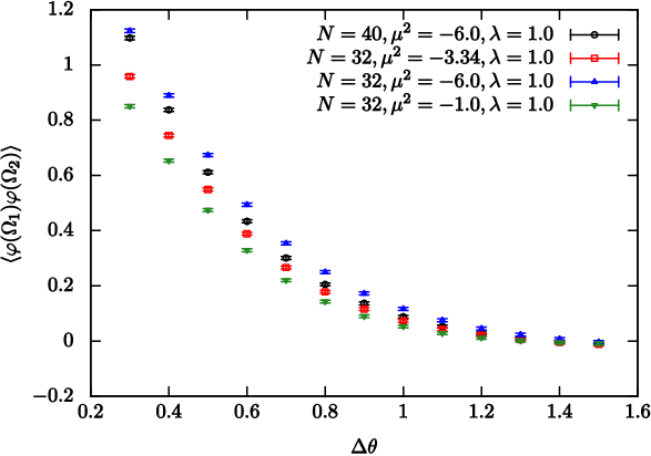
Figure 2: ⟨φ⁡(Ω1)​φ​(Ω2)⟩\left\langle\varphi(\Omega_{1})\varphi(\Omega_{2})\right\rangle at λ=1.0\lambda=1.0 is plotted against Δ​θ\Delta\theta. Circles represent the data for N=40N=40 and μ2=−6.0\mu^{2}=-6.0, while squares, triangles, and inverted triangles represent the data for N=32N=32 and μ2=−3.34,−6.0,−1.0\mu^{2}=-3.34,-6.0,-1.0, respectively.
Refer to caption
Figure 3: ⟨φ⁡(Ω1)​φ​(Ω2)⟩\left\langle\varphi(\Omega_{1})\varphi(\Omega_{2})\right\rangle at N=40N=40, μ2=−6.0\mu^{2}=-6.0, and λ=1.0\lambda=1.0 is plotted against Δ​θ\Delta\theta (circles). ζ32→40​⟨φ⁡(Ω1)​φ​(Ω2)⟩\zeta_{32\rightarrow 40}\left\langle\varphi(\Omega_{1})\varphi(\Omega_{2})\right\rangle with ζ32→40=1.263​(8)\zeta_{32\rightarrow 40}=1.263(8) at N=32N=32, μ2=−3.34\mu^{2}=-3.34, and λ=1.0\lambda=1.0 is also plotted against Δ​θ\Delta\theta (squares).
Refer to caption
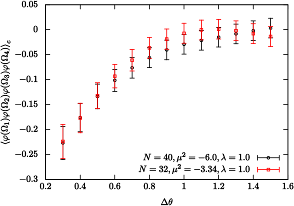
Figure 4: ⟨φ⁡(Ω1)​φ​(Ω2)​φ​(Ω3)​φ​(Ω4)⟩c\left\langle\varphi(\Omega_{1})\varphi(\Omega_{2})\varphi(\Omega_{3})\varphi(\Omega_{4})\right\rangle_{c} at N=40N=40, μ2=−6.0\mu^{2}=-6.0, and λ=1.0\lambda=1.0 is plotted against Δ​θ\Delta\theta (circles). ζ32→402​⟨φ⁡(Ω1)​φ​(Ω2)​φ​(Ω3)​φ​(Ω4)⟩c\zeta_{32\rightarrow 40}^{2}\left\langle\varphi(\Omega_{1})\varphi(\Omega_{2})\varphi(\Omega_{3})\varphi(\Omega_{4})\right\rangle_{c} with ζ32→402=1.595\zeta_{32\rightarrow 40}^{2}=1.595 at N=32N=32, μ2=−3.34\mu^{2}=-3.34, and λ=1.0\lambda=1.0 is also plotted against Δ​θ\Delta\theta (squares).

First, we simulate at N=40N=40 and μ2=−6.0\mu^{2}=-6.0. Then, we simulate at N=32N=32 for various values of μ2\mu^{2}. In Fig.2, we plot

⟨φ⁡(Ω1)​φ​(Ω2)⟩=Z⁡⟨φr​(Ω1)​φr​(Ω2)⟩\left\langle\varphi(\Omega_{1})\varphi(\Omega_{2})\right\rangle=Z\left\langle\varphi_{r}(\Omega_{1})\varphi_{r}(\Omega_{2})\right\rangle (3.12)

against Δ​θ\Delta\theta at N=40N=40 and μ2=−6.0\mu^{2}=-6.0 and at N=32N=32 and typical values of μ2\mu^{2}, −6.0,−3.34,−1.0-6.0,-3.34,-1.0. We find that the data for N=32N=32 and μ2=−3.34\mu^{2}=-3.34 agree with the ones for N=40N=40 and μ2=−6.0\mu^{2}=-6.0 if the former are multiplied by a constant and that this is not the case for the data for N=32N=32 and μ2=−6.0,−1.0\mu^{2}=-6.0,-1.0. We determined the above constant as ζ32→40=Z⁡(40)Z⁡(32)=1.263​(8)\zeta_{32\rightarrow 40}=\frac{Z(40)}{Z(32)}=1.263(8) by using the least-squares method. In Fig.3, we plot ⟨φ⁡(Ω1)​φ​(Ω2)⟩\left\langle\varphi(\Omega_{1})\varphi(\Omega_{2})\right\rangle at N=40N=40 and μ2=−6.0\mu^{2}=-6.0 and ζ32→40​⟨φ⁡(Ω1)​φ​(Ω2)⟩\zeta_{32\rightarrow 40}\left\langle\varphi(\Omega_{1})\varphi(\Omega_{2})\right\rangle at N=32N=32 and μ2=−3.34\mu^{2}=-3.34 against Δ​θ\Delta\theta. We indeed see that the data for N=32N=32 agree nicely with the ones for N=40N=40. This implies that the renormalized 2-point functions at N=32N=32 and N=40N=40 agree.

Furthermore, in Fig.4, we plot ⟨φ⁡(Ω1)​φ​(Ω2)​φ​(Ω3)​φ​(Ω4)⟩c\left\langle\varphi(\Omega_{1})\varphi(\Omega_{2})\varphi(\Omega_{3})\varphi(\Omega_{4})\right\rangle_{c} at N=40N=40 and μ2=−6.0\mu^{2}=-6.0 and ζ32→402​⟨φ⁡(Ω1)​φ​(Ω2)​φ​(Ω3)​φ​(Ω4)⟩c\zeta_{32\rightarrow 40}^{2}\left\langle\varphi(\Omega_{1})\varphi(\Omega_{2})\varphi(\Omega_{3})\varphi(\Omega_{4})\right\rangle_{c} at N=32N=32 and μ2=−3.34\mu^{2}=-3.34 against Δ​θ\Delta\theta. We again see a nice agreement between the data for N=32N=32 and the ones for N=40N=40, which means that the renormalized connected 4-point functions at N=32N=32 agree with those at N=40N=40. We do not see the above agreement of the correlation functions for m=1,2m=1,2 in (3.11). We consider this to be attributed to the UV cutoff.

The above results strongly suggest that the correlation functions are made independent of NN up to a wave function renormalization by tuning μ2\mu^{2} and that the theory is nonperturbatively renormalizable in the ordinary sense.

3.3 Tuning λ\lambda

In this subsection, we renormalize the theory by tuning λ\lambda. We fix μ2\mu^{2} at −6.0-6.0.

Refer to caption
Figure 5: ⟨φ⁡(Ω1)​φ​(Ω2)⟩\left\langle\varphi(\Omega_{1})\varphi(\Omega_{2})\right\rangle at μ2=−6.0\mu^{2}=-6.0 is plotted against Δ​θ\Delta\theta. Circles represent the data for N=40N=40 and λ=1.0\lambda=1.0, while squares, triangles, and inverted triangles represent the data for N=32N=32 and λ=1.234,1.0,2.0\lambda=1.234,1.0,2.0 , respectively.
Refer to caption
Figure 6: ⟨φ⁡(Ω1)​φ​(Ω2)⟩\left\langle\varphi(\Omega_{1})\varphi(\Omega_{2})\right\rangle at N=40N=40, μ2=−6.0\mu^{2}=-6.0, and λ=1.0\lambda=1.0 is plotted against Δ​θ\Delta\theta (circles). ζ′32→40​⟨φ⁡(Ω1)​φ​(Ω2)⟩{\zeta^{\prime}}_{32\rightarrow 40}\left\langle\varphi(\Omega_{1})\varphi(\Omega_{2})\right\rangle with ζ′32→40=1.129​(8){\zeta^{\prime}}_{32\rightarrow 40}=1.129(8) at N=32N=32, μ2=−6.0\mu^{2}=-6.0, and λ=1.234\lambda=1.234 is also plotted against Δ​θ\Delta\theta (squares).
Refer to caption
Figure 7: ⟨φ⁡(Ω1)​φ​(Ω2)​φ​(Ω3)​φ​(Ω4)⟩c\left\langle\varphi(\Omega_{1})\varphi(\Omega_{2})\varphi(\Omega_{3})\varphi(\Omega_{4})\right\rangle_{c} at N=40N=40, μ2=−6.0\mu^{2}=-6.0, and λ=1.0\lambda=1.0 is plotted against Δ​θ\Delta\theta, where circles represent the data. ζ′32→402​⟨φ⁡(Ω1)​φ​(Ω2)​φ​(Ω3)​φ​(Ω4)⟩c{\zeta^{\prime}}_{32\rightarrow 40}^{2}\left\langle\varphi(\Omega_{1})\varphi(\Omega_{2})\varphi(\Omega_{3})\varphi(\Omega_{4})\right\rangle_{c} with ζ′32→402=1.275{\zeta^{\prime}}_{32\rightarrow 40}^{2}=1.275 at N=32N=32, μ2=−6.0\mu^{2}=-6.0, and λ=1.234\lambda=1.234 is also plotted against Δ​θ\Delta\theta, where squares represent the data.

We simulate at N=32N=32 for various values of λ\lambda. In Fig.5, we plot

⟨φ⁡(Ω1)​φ​(Ω2)⟩=Z⁡⟨φr​(Ω1)​φr​(Ω2)⟩\left\langle\varphi(\Omega_{1})\varphi(\Omega_{2})\right\rangle=Z\left\langle\varphi_{r}(\Omega_{1})\varphi_{r}(\Omega_{2})\right\rangle (3.13)

against Δ​θ\Delta\theta at N=40N=40 and λ=1.0\lambda=1.0 and at N=32N=32 and typical values of λ\lambda, 1.0,1.234,2.01.0,1.234,2.0. We find that the data for N=32N=32 and λ=1.234\lambda=1.234 agree with the ones for N=40N=40 and λ=1.0\lambda=1.0 if the former are multiplied by a constant ζ′32→40=Z⁡(40)Z⁡(32)=1.129​(8){\zeta^{\prime}}_{32\rightarrow 40}=\frac{Z(40)}{Z(32)}=1.129(8) and that this is not the case for the data for N=32N=32 and λ=1.0,2.0\lambda=1.0,2.0. In Fig.6, we plot ⟨φ⁡(Ω1)​φ​(Ω2)⟩\left\langle\varphi(\Omega_{1})\varphi(\Omega_{2})\right\rangle at N=40N=40 and λ=1.0\lambda=1.0 and ζ′32→40​⟨φ⁡(Ω1)​φ​(Ω2)⟩{\zeta^{\prime}}_{32\rightarrow 40}\left\langle\varphi(\Omega_{1})\varphi(\Omega_{2})\right\rangle at N=32N=32 and λ=1.234\lambda=1.234 against Δ​θ\Delta\theta. As in the previous section, we see that the data for N=32N=32 agree nicely with the ones for N=40N=40. This implies that the renormalized 2-point functions at N=32N=32 and N=40N=40 agree.

Furthermore, in Fig.7, we plot ⟨φ⁡(Ω1)​φ​(Ω2)​φ​(Ω3)​φ​(Ω4)⟩c\left\langle\varphi(\Omega_{1})\varphi(\Omega_{2})\varphi(\Omega_{3})\varphi(\Omega_{4})\right\rangle_{c} at N=40N=40 and λ=1.0\lambda=1.0 and ζ′32→402​⟨φ⁡(Ω1)​φ​(Ω2)​φ​(Ω3)​φ​(Ω4)⟩c{\zeta^{\prime}}_{32\rightarrow 40}^{2}\left\langle\varphi(\Omega_{1})\varphi(\Omega_{2})\varphi(\Omega_{3})\varphi(\Omega_{4})\right\rangle_{c} at N=32N=32 and λ=1.234\lambda=1.234 against Δ​θ\Delta\theta. We again see a nice agreement between the data for N=32N=32 and the ones for N=40N=40, which means that the renormalized connected 4-point functions at N=32N=32 agree with those at N=40N=40.

The above results strongly suggest that the theory is also nonperturbatively renormalized by tuning λ\lambda in the sense that the renormalized correlation functions are independent of NN.

The results in the previous and present sections imply that the theory is renormalized by tuning a parameter; namely, it is universal up to a parameter fine-tuning.

4 Critical behavior of correlation functions

In this section, we examine the 2-point and 4-point correlation functions on the phase boundary. We fix NN at 24 in this section.

We introduce a stereographic projection defined by

z=R​tan⁡θ2​ei​φ,z=R\tan\frac{\theta}{2}e^{i\varphi}\ , (4.1)

which maps a sphere with the radius RR to the complex plane. Here we fix RR at 11 without loss of generality. We calculate the 2-point correlation function

⟨φ⁡(zm)​φ​(1)⟩\langle\varphi(z_{m})\varphi(1)\rangle (4.2)

and the connected 4-point correlation function

⟨φ⁡(zm)​φ​(1)​φ​(ei​π3)​φ​(ei​5​π3)⟩c,\langle\varphi(z_{m})\varphi(1)\varphi(e^{i\frac{\pi}{3}})\varphi(e^{i\frac{5\pi}{3}})\rangle_{c}\ , (4.3)

where

zm=tan⁡[12​(π2+0.1​m)]z_{m}=\tan\left[\frac{1}{2}\left(\frac{\pi}{2}+0.1m\right)\right] (4.4)

with mm taken from11 to 1515. See Fig. 1 with φ^=π/3\hat{\varphi}=\pi/3.

The renormalized 2-point correlation function ⟨φr​(zm)​φr​(1)⟩\langle\varphi_{r}(z_{m})\varphi_{r}(1)\rangle and the renormalized connected 4-point correlation function ⟨φr​(zm)​φr​(1)​φr​(ei​π3)​φr​(ei​5​π3)⟩c\langle\varphi_{r}(z_{m})\varphi_{r}(1)\varphi_{r}(e^{i\frac{\pi}{3}})\varphi_{r}(e^{i\frac{5\pi}{3}})\rangle_{c} are defined by

⟨φ⁡(zm)​φ​(1)⟩\displaystyle\langle\varphi(z_{m})\varphi(1)\rangle =Z⁡⟨φr​(zm)​φr​(1)⟩,\displaystyle=Z\langle\varphi_{r}(z_{m})\varphi_{r}(1)\rangle\ , (4.5)
⟨φ⁡(zm)​φ​(1)​φ​(ei​π3)​φ​(ei​5​π3)⟩c\displaystyle\langle\varphi(z_{m})\varphi(1)\varphi(e^{i\frac{\pi}{3}})\varphi(e^{i\frac{5\pi}{3}})\rangle_{c} =Z2​⟨φr​(zm)​φr​(1)​φr​(ei​π3)​φr​(ei​5​π3)⟩c.\displaystyle=Z^{2}\langle\varphi_{r}(z_{m})\varphi_{r}(1)\varphi_{r}(e^{i\frac{\pi}{3}})\varphi_{r}(e^{i\frac{5\pi}{3}})\rangle_{c}\ . (4.6)
Refer to caption
Figure 8: log⁡⟨φ⁡(zm)​φ​(1)⟩\log\langle\varphi(z_{m})\varphi(1)\rangle at N=24N=24 is plotted against log⁡|z−1|\log|z-1|. The data for (μ2,λ)=(−10.801,0.5),(−12.810,0.6),(−14.925,0.7)(\mu^{2},\lambda)=(-10.801,0.5),(-12.810,0.6),(-14.925,0.7) are represented by the circles, the squares, and the triangles, respectively.
Refer to caption
Figure 9: log⁡⟨φ⁡(zm)​φ​(1)​φr​(ei​π3)​φr​(ei​5​π3)⟩c\log\langle\varphi(z_{m})\varphi(1)\varphi_{r}(e^{i\frac{\pi}{3}})\varphi_{r}(e^{i\frac{5\pi}{3}})\rangle_{c} at N=24N=24 is plotted against log⁡|z−1|\log|z-1|. The data for (μ2,λ)=(−10.801,0.5),(−12.810,0.6),(−14.925,0.7)(\mu^{2},\lambda)=(-10.801,0.5),(-12.810,0.6),(-14.925,0.7) are represented by the circles, the squares, and the triangles, respectively.

Here, in order to see a connection to a CFT, we use a log-log plot. We plot log⁡⟨φ⁡(zm)​φ​(1)⟩\log\langle\varphi(z_{m})\varphi(1)\rangle and log⁡⟨φ⁡(zm)​φ​(1)​φ​(ei​π3)​φ​(ei​5​π3)⟩c\log\langle\varphi(z_{m})\varphi(1)\varphi(e^{i\frac{\pi}{3}})\varphi(e^{i\frac{5\pi}{3}})\rangle_{c} against log⁡|z−1|\log|z-1| for (μ2,λ)=(−10.801,0.5),(−12.810,0.6)(\mu^{2},\lambda)=(-10.801,0.5),(-12.810,0.6), (−14.925,0.7)(-14.925,0.7) in Figs.8 and 9, respectively.

Refer to caption
Figure 10: The susceptibility χ\chi at N=24N=24 is plotted against −μ2-\mu^{2}. The data for λ=0.5,0.6,0.7\lambda=0.5,0.6,0.7 are represented by the circles, the squares, and the triangles, respectively. The peaks of χ\chi for λ=0.5,0.6,0.7\lambda=0.5,0.6,0.7 exist around μ2=−10.8,−12.8,−14.8\mu^{2}=-10.8,-12.8,-14.8, respectively.
Refer to caption
Figure 11: log⁡⟨φ⁡(zm)​φ​(1)⟩\log\langle\varphi(z_{m})\varphi(1)\rangle at N=24N=24 is plotted against log⁡|z−1|\log|z-1|. The data for (μ2,λ)=(−10.801,0.5)(\mu^{2},\lambda)=(-10.801,0.5) are the same as in Fig. 8. The data for (μ2,λ)=(−12.810,0.6),(−14.925,0.7)(\mu^{2},\lambda)=(-12.810,0.6),(-14.925,0.7) are simultaneously shifted by α0.6→0.5=−0.015​(1)\alpha_{0.6\to 0.5}=-0.015(1) and α0.7→0.5=−0.056​(1)\alpha_{0.7\to 0.5}=-0.056(1), respectively, in the vertical direction. The data for (μ2,λ)=(−10.801,0.5),(−12.810,0.6),(−14.925,0.7)(\mu^{2},\lambda)=(-10.801,0.5),(-12.810,0.6),(-14.925,0.7) are represented by the circles, the squares, and the triangles, respectively. The dashed line is a fit of seven data points (from the second point to the eighth point) of log⁡⟨φ⁡(zm)​φ​(1)⟩\log\langle\varphi(z_{m})\varphi(1)\rangle at (μ2,λ)=(−10.801,0.5)(\mu^{2},\lambda)=(-10.801,0.5) to −u​log⁡|z−1|+v-u\log|z-1|+v with u=0.149​(2)u=0.149(2) and v=1.887​(1)v=1.887(1).
Refer to caption
Figure 12: log⁡⟨φ⁡(zm)​φ​(1)​φ​(ei​π3)​φ​(ei​5​π3)⟩c\log\langle\varphi(z_{m})\varphi(1)\varphi(e^{i\frac{\pi}{3}})\varphi(e^{i\frac{5\pi}{3}})\rangle_{c} at N=24N=24 is plotted against log⁡|z−1|\log|z-1|. The data for (μ2,λ)=(−10.801,0.5)(\mu^{2},\lambda)=(-10.801,0.5) are the same as in Fig. 9, while the data for (μ2,λ)=(−12.810,0.6),(−14.925,0.7)(\mu^{2},\lambda)=(-12.810,0.6),(-14.925,0.7) are simultaneously shifted by 2​α0.6→0.52\alpha_{0.6\to 0.5} and 2​α0.7→0.52\alpha_{0.7\to 0.5}, respectively, in the vertical direction. The data for (μ2,λ)=(−10.801,0.5)(\mu^{2},\lambda)=(-10.801,0.5), (−12.810,0.6),(−14.925,0.7)(-12.810,0.6),(-14.925,0.7) are represented by the circles, the squares, and the triangles, respectively.

We also define the susceptibility χ\chi that is an order parameter for the Z2Z_{2} symmetry by

χ=⟨(1N​Tr​Φ)2⟩−⟨1N​|Tr​Φ|⟩2.\chi=\left\langle\left(\frac{1}{N}\mbox{Tr}\Phi\right)^{2}\right\rangle-\left\langle\frac{1}{N}\left|\mbox{Tr}\Phi\right|\right\rangle^{2}\ . (4.7)

In Fig.10, we plot χ\chi against −μ2-\mu^{2} for each value of λ\lambda, 0.5,0.6,0.70.5,0.6,0.7. The critical values of −μ2-\mu^{2}, −μc2-\mu^{2}_{c}, that give the peaks of χ\chi correspond to the phase transition points where symmetry breaking of the Z2Z_{2} symmetry occurs: the Z2Z_{2} symmetry is broken for −μ2>−μc2-\mu^{2}>-\mu^{2}_{c}, while it is unbroken for −μ2<−μc2-\mu^{2}<-\mu^{2}_{c}. We find that peaks of χ\chi for λ=0.5,0.6,0.7\lambda=0.5,0.6,0.7 exist around μ2=−10.8,−12.8,−14.8\mu^{2}=-10.8,-12.8,-14.8, respectively. We tune the values of μ2\mu^{2} around the above values such that the 2-point and 4-point correlation functions for different λ\lambda agree up to a wave function renormalization. We shift the data of the 2-point correlation functions for (μ2,λ)=(−12.810,0.6),(−14.925,0.7)(\mu^{2},\lambda)=(-12.810,0.6),(-14.925,0.7) simultaneously in the vertical direction by α0.6→0.5=log⁡[Z⁡(λ=0.5)/Z⁡(λ=0.6)]=−0.015​(1)\alpha_{0.6\to 0.5}=\log[Z(\lambda=0.5)/Z(\lambda=0.6)]=-0.015(1) and α0.7→0.5=−0.056​(1)\alpha_{0.7\to 0.5}=-0.056(1), respectively, and plot the shifted data in Fig.11. We also shift the data of the 4-point correlation functions for (μ2,λ)=(−12.810,0.6),(−14.925,0.7)(\mu^{2},\lambda)=(-12.810,0.6),(-14.925,0.7) simultaneously by 2​α0.6→0.52\alpha_{0.6\to 0.5} and 2​α0.7→0.52\alpha_{0.7\to 0.5}, respectively, and plot the shifted data in Fig.12. We see a good agreement of both the shifted 2-point and 4-point correlation functions. These shifts correspond to a wave function renormalization. Furthermore, we see that the above tuned values of μ2\mu^{2} are consistent with the critical values of μ2\mu^{2} read off from Fig.10. Thus, the agreement of the correlation functions implies that the theories are universal on the phase boundary as in ordinary field theories. We do not see the above agreement of the correlation functions in either the UV region with m=1,2m=1,2, or the IR region with m=14,15m=14,15. We consider the disagreement in the latter region to be caused by an IR cutoff that is introduced when the theory on the fuzzy sphere is mapped to a theory on the plane with infinite volume.

Finally, we examine a connection of the present theory to a CFT. In Fig.11, we fit seven data points (m=4,…,10m=4,\ldots,10) of log⁡⟨φ⁡(zm)​φ​(1)⟩\log\langle\varphi(z_{m})\varphi(1)\rangle at (μ2,λ)=(−10.801,0.5)(\mu^{2},\lambda)=(-10.801,0.5) to −u​log⁡|z−1|+v-u\log|z-1|+v and obtain u=0.149​(2)u=0.149(2) and v=1.887​(1)v=1.887(1). This implies that the 2-point correlation function behaves as

⟨φ⁡(z)​φ​(1)⟩=ev|z−1|u\langle\varphi(z)\varphi(1)\rangle=\frac{e^{v}}{|z-1|^{u}} (4.8)

for m=4,…,10m=4,\ldots,10. In CFTs, the 2-point correlation function behaves as

⟨𝒪⁡(z)​𝒪​(z′)⟩∼1|z−z′|2​Δ,\left\langle\mathcal{O}(z)\mathcal{O}(z^{\prime})\right\rangle\sim\frac{1}{|z-z^{\prime}|^{2\Delta}}\ , (4.9)

where the Δ\Delta is the scaling dimension of the operator 𝒪⁡(z)\mathcal{O}(z). Thus, the theory on the phase boundary behaves as a CFT in the UV region. In the IR region with 11≤m≤1311\leq m\leq 13, our 2-point correlation function deviates universally from that in the CFT. In addition, in a further UV region with m=3m=3, it also deviates universally. These deviations are considered to be an effect of the UV/IR mixing. It is nontrivial that we observe the behavior of the CFT because field theories on noncommutative spaces are non-local ones.

5 Conclusion and discussion

In this paper, we have studied renormalization in the scalar filed theory on the fuzzy sphere by Monte Carlo simulation. We showed that the 2-point and 4-point correlation functions in the disordered phase are made independent of the UV cutoff up to the wave function renormalization by tuning the mass parameter or the coupling constant. This strongly suggests that the theory can be renormalized nonperturbatively in the ordinary sense and that the theory is universal up to a parameter fine-tuning.

We also examined the 2-point and 4-point correlation functions on the phase boundary beyond which the Z2Z_{2} symmetry is spontaneously broken. We found that the 2-point and 4-point correlation functions at different points on the boundary agree up to the wave function renormalization. This implies that the critical theory is universal, which is consistent with the above universality in the disordered phase, because the phase boundary is obtained by a parameter fine-tuning. Furthermore, we observed that the 2-point correlation functions behave as those in a CFT at short distances and deviate universally from those at long distances. The latter is considered to be due to the UV/IR mixing.

The CFT that we observed at short distances seems to differ from the critical Ising model, because the value of uu in (4.8) disagrees with 2​Δ2\Delta, where Δ\Delta is the scaling dimension of the spin operator, 1/81/8. This suggests that the universality classes of the scalar field theory on the fuzzy sphere are totally different from those of an ordinary field theory33 3 It should be noted that the scaling dimension that we obtained, Δ≃0.075=3/40\Delta\simeq 0.075=3/40, coincides with that of the spin operator in the tricritical Ising model, which is the (4,5)(4,5) unitary minimal model..

Indeed, it was reported in [5, 6, 7, 8, 9] that there exists a novel phase in the theory on the fuzzy sphere that is called the nonuniformly ordered phase [24, 25]. We hope to elucidate the universality classes by studying renormalization in the whole phase diagram.

Acknowledgements

Numerical computation was carried out on the XC40 at YITP at Kyoto University and FX10 at the University of Tokyo. The work of A.T. is supported in part by a Grant-in-Aid for Scientific Research (No. 15K05046) from JSPS.

Appendix: Bloch coherent state and Berezin symbol

In this appendix, we summarize the basic properties of the Bloch coherent state [23] and the Berezin symbol[22].

We use a standard basis |j​m⟩|jm\rangle (m=−j,−j+1,…,j)(m=-j,-j+1,\ldots,j) for the spin-jj (=(N−1)/2)(=(N-1)/2) representation of the S​U​(2)SU(2) algebra. The action of LiL_{i} on the basis is given by

L±​|j​m⟩\displaystyle L_{\pm}|jm\rangle =(j∓m)​(j±m+1)​|j​m±1⟩,\displaystyle=\sqrt{(j\mp m)(j\pm m+1)}|jm\pm 1\rangle,
L3​|j​m⟩\displaystyle L_{3}|jm\rangle =m​|j​m⟩,\displaystyle=m|jm\rangle\ , (A.1)

where L±=L1±i​L2L_{\pm}=L_{1}\pm iL_{2}. The highest-weight state |j​j⟩|jj\rangle is considered to correspond to the north pole. Thus, the state |Ω⟩|\Omega\rangle that corresponds to a point Ω=(θ,φ)\Omega=(\theta,\varphi) is obtained by acting a rotation operator on |j​j⟩|jj\rangle:

|Ω⟩=ei​θ​(sin⁡φ​L1−cos⁡φ​L2)​|j​j⟩.|\Omega\rangle=e^{i\theta(\sin\varphi L_{1}-\cos\varphi L_{2})}|jj\rangle\ . (A.2)

(A.2) implies that

ni​Li​|Ω⟩=j⁡|Ω⟩,n_{i}L_{i}|\Omega\rangle=j|\Omega\rangle\ , (A.3)

where n→=(sin⁡θ​cos⁡φ,sin⁡θ​sin⁡φ,cos⁡θ)\vec{n}=(\sin\theta\cos\varphi,\sin\theta\sin\varphi,\cos\theta). It is easy to show from (A.3) that |Ω⟩|\Omega\rangle minimizes ∑i(Δ​Li)2\sum_{i}(\Delta L_{i})^{2} with (Δ​Li)2(\Delta L_{i})^{2} being the standard deviation of LiL_{i}.

It is convenient to introduce the stereographic projection, z=R​tan⁡θ2​ei​φz=R\tan\frac{\theta}{2}e^{i\varphi}. Then, (A.2) is rewritten as

|Ω⟩=ez​L−/Re−L3​log⁡(1+|z/R|2)e−z¯L+/R|jj⟩,|\Omega\rangle=e^{zL_{-}/R}e^{-L_{3}\log(1+|z/R|^{2})}e^{-\bar{z}L_{+}/R}|jj\rangle\ , (A.4)

which gives an explicit form of |Ω⟩|\Omega\rangle as

|Ω⟩=∑m=−jj(2​jj+m)12​(cos⁡θ2)j+m​(sin⁡θ2)j−m​ei⁡(j−m)​φ​|j​m⟩.|\Omega\rangle=\sum_{m=-j}^{j}\left(\begin{array}[]{c}2j\\ j+m\end{array}\right)^{\frac{1}{2}}\left(\cos\frac{\theta}{2}\right)^{j+m}\left(\sin\frac{\theta}{2}\right)^{j-m}e^{i(j-m)\varphi}|jm\rangle\ . (A.5)

By using (A.5), one can easily show the following relations:

⟨Ω1|Ω2⟩=(cos⁡θ12​cos⁡θ22+ei⁡(φ2−φ1)​sin⁡θ12​sin⁡θ22)2​j,\displaystyle\langle\Omega_{1}|\Omega_{2}\rangle=\left(\cos\frac{\theta_{1}}{2}\cos\frac{\theta_{2}}{2}+e^{i(\varphi_{2}-\varphi_{1})}\sin\frac{\theta_{1}}{2}\sin\frac{\theta_{2}}{2}\right)^{2j}\ , (A.6)
|⟨Ω1|Ω2⟩|=(cos⁡χ2)2​j​with​χ=arccos⁡(n→1⋅n→2),\displaystyle|\langle\Omega_{1}|\Omega_{2}\rangle|=\left(\cos\frac{\chi}{2}\right)^{2j}\;\;\mbox{with}\;\;\chi=\arccos(\vec{n}_{1}\cdot\vec{n}_{2})\ , (A.7)
2​j+14​π​∫d​Ω​|Ω⟩​⟨Ω|=1.\displaystyle\frac{2j+1}{4\pi}\int d\Omega\ |\Omega\rangle\langle\Omega|=1\ . (A.8)

(A.7) implies that the width of the Bloch coherent state is Rj\frac{R}{\sqrt{j}} for large jj.

Denoting the Bloch coherent state |Ω⟩|\Omega\rangle by |z⟩|z\rangle, we rewrite (A.5) and (A.8) as

|z⟩=(z/R1+|z/R|2)j​∑m=−jj(2​jj+m)12​Rmzm​|j​m⟩,\displaystyle|z\rangle=\left(\frac{z/R}{1+|z/R|^{2}}\right)^{j}\sum_{m=-j}^{j}\left(\begin{array}[]{c}2j\\ j+m\end{array}\right)^{\frac{1}{2}}\frac{R^{m}}{z^{m}}|jm\rangle\ ,
2​j+14​π​4​R2​∫d2​z(1+|z/R|2)2​|z⟩​⟨z|=1,\displaystyle\frac{2j+1}{4\pi}4R^{2}\int\frac{d^{2}z}{(1+|z/R|^{2})^{2}}\ |z\rangle\langle z|=1\ , (A.11)

respectively.

The Berezin symbol for a matrix AA with the matrix size 2​j+12j+1 is defined by

fA​(Ω)\displaystyle f_{A}(\Omega) =fA​(z,z¯)\displaystyle=f_{A}(z,\bar{z})
=⟨Ω|A|Ω⟩\displaystyle=\langle\Omega|A|\Omega\rangle
=⟨z|A|z⟩.\displaystyle=\langle z|A|z\rangle\ . (A.12)

By using (A.5), it is easy to show that

f[Li,A]​(Ω)=ℒi​fA​(Ω).f_{[L_{i},A]}(\Omega)={\cal L}_{i}f_{A}(\Omega)\ . (A.13)

(A.8) implies that

1N​Tr​(A)=∫d​Ω4​π​fA​(Ω).\frac{1}{N}\mbox{Tr}(A)=\int\frac{d\Omega}{4\pi}f_{A}(\Omega)\ . (A.14)

The definition of the star product for AA and BB is

fA⋆fB​(Ω)=fA⋆fB​(z,z¯)=⟨Ω|A​B|Ω⟩=⟨z|A​B|z⟩.f_{A}\star f_{B}(\Omega)=f_{A}\star f_{B}(z,\bar{z})=\langle\Omega|AB|\Omega\rangle=\langle z|AB|z\rangle\ . (A.15)

Here let us consider a quantity

⟨w|A|z⟩⟨w|z⟩,\frac{\langle w|A|z\rangle}{\langle w|z\rangle}\ , (A.16)

which is holomorphic in zz and anti-holomorphic in ww. Then, one can deform this quantity as follows:

⟨w|A|z⟩⟨w|z⟩\displaystyle\frac{\langle w|A|z\rangle}{\langle w|z\rangle} =e−w​∂∂z​⟨w|A|z+w⟩⟨w|z+w⟩\displaystyle=e^{-w\frac{\partial}{\partial z}}\frac{\langle w|A|z+w\rangle}{\langle w|z+w\rangle}
=e−w​∂∂z​ez​∂∂w​⟨w|A|w⟩⟨w|w⟩\displaystyle=e^{-w\frac{\partial}{\partial z}}e^{z\frac{\partial}{\partial w}}\frac{\langle w|A|w\rangle}{\langle w|w\rangle}
=e−w​∂∂z​ez​∂∂w​⟨w|A|w⟩\displaystyle=e^{-w\frac{\partial}{\partial z}}e^{z\frac{\partial}{\partial w}}\langle w|A|w\rangle
=e−w​∂∂z​ez​∂∂w​fA​(w,w¯).\displaystyle=e^{-w\frac{\partial}{\partial z}}e^{z\frac{\partial}{\partial w}}f_{A}(w,\bar{w})\ . (A.17)

Similarly, one obtains

⟨z|A|w⟩⟨z|w⟩=e−w¯​∂∂z¯​ez¯​∂∂w¯​fA​(w,w¯).\frac{\langle z|A|w\rangle}{\langle z|w\rangle}=e^{-\bar{w}\frac{\partial}{\partial\bar{z}}}e^{\bar{z}\frac{\partial}{\partial\bar{w}}}f_{A}(w,\bar{w})\ . (A.18)

By using (A.11), (A.17), and (A.18), one can express the star product as

fA⋆fB​(w,w¯)\displaystyle f_{A}\star f_{B}(w,\bar{w}) =⟨w|A​B|w⟩\displaystyle=\langle w|AB|w\rangle
=2​j+14​π​4​R2​∫d2​z(1+|z/R|2)2​⟨w|A|z⟩⟨w|z⟩​⟨z|B|w⟩⟨z|w⟩​|⟨w|z⟩|2\displaystyle=\frac{2j+1}{4\pi}4R^{2}\int\frac{d^{2}z}{(1+|z/R|^{2})^{2}}\frac{\langle w|A|z\rangle}{\langle w|z\rangle}\frac{\langle z|B|w\rangle}{\langle z|w\rangle}|\langle w|z\rangle|^{2}
=2​j+14​π​4​R2​∫d2​z(1+|z/R|2)2​(e−w​∂∂z​ez​∂∂w​fA​(w,w¯))​(e−w¯​∂∂z¯​ez¯​∂∂w¯​fB​(w,w¯))​|⟨w|z⟩|2,\displaystyle=\frac{2j+1}{4\pi}4R^{2}\int\frac{d^{2}z}{(1+|z/R|^{2})^{2}}(e^{-w\frac{\partial}{\partial z}}e^{z\frac{\partial}{\partial w}}f_{A}(w,\bar{w}))(e^{-\bar{w}\frac{\partial}{\partial\bar{z}}}e^{\bar{z}\frac{\partial}{\partial\bar{w}}}f_{B}(w,\bar{w}))|\langle w|z\rangle|^{2}\ , (A.19)

which indicates that the star product is noncommutative and non-local. Furthermore, one can easily show that in the j→∞j\rightarrow\infty limit

2​j+14​π​4​R2(1+|z/R|2)2​|⟨w|z⟩|2→δ2​(z−w).\frac{2j+1}{4\pi}\frac{4R^{2}}{(1+|z/R|^{2})^{2}}|\langle w|z\rangle|^{2}\rightarrow\delta^{2}(z-w)\ . (A.20)

This implies that the star product coincides with the ordinary product in the j→∞j\rightarrow\infty limit. Namely,

fA⋆fB​(w,w¯)→fA​(w,w¯)​fB​(w,w¯)f_{A}\star f_{B}(w,\bar{w})\rightarrow f_{A}(w,\bar{w})f_{B}(w,\bar{w}) (A.21)

or

fA⋆fB​(Ω)→fA​(Ω)​fB​(Ω).f_{A}\star f_{B}(\Omega)\rightarrow f_{A}(\Omega)f_{B}(\Omega)\ . (A.22)

We see from (A.13), (A.14), and (A.22) that the theory (2.1) reduces to that of (2.4) in the N→∞N\rightarrow\infty limit at the classical level if one identifies fΦ​(Ω)f_{\Phi}(\Omega) with ϕ⁡(Ω)\phi(\Omega). However, the authors of [3, 4] showed that the one-loop effective action in (2.1) differs from that in (2.4) by finite and non-local terms since the UV cutoff NN is kept finite in calculating loop corrections. This phenomenon is sometimes called the UV/IR anomaly.

References

  • [1] M. R. Douglas and N. A. Nekrasov, Rev. Mod. Phys. 73, 977 (2001) [hep-th/0106048].
  • [2] S. Minwalla, M. Van Raamsdonk and N. Seiberg, JHEP 0002, 020 (2000) [hep-th/9912072].
  • [3] C. S. Chu, J. Madore and H. Steinacker, JHEP 0108, 038 (2001) [hep-th/0106205].
  • [4] H. C. Steinacker, Nucl. Phys. B 910, 346 (2016) [arXiv:1606.00646 [hep-th]].
  • [5] X. Martin, JHEP 0404, 077 (2004) [hep-th/0402230].
  • [6] M. Panero, JHEP 0705, 082 (2007) [hep-th/0608202].
  • [7] M. Panero, SIGMA 2, 081 (2006) [hep-th/0609205].
  • [8] F. Garcia Flores, X. Martin and D. O’Connor, Int. J. Mod. Phys. A 24, 3917 (2009) [arXiv:0903.1986 [hep-lat]].
  • [9] C. R. Das, S. Digal and T. R. Govindarajan, Mod. Phys. Lett. A 23, 1781 (2008) [arXiv:0706.0695 [hep-th]].
  • [10] K. Hatakeyama and A. Tsuchiya, PTEP 2017, no. 6, 063B01 (2017) [arXiv:1704.01698 [hep-th]].
  • [11] S. Kawamoto and T. Kuroki, JHEP 1506, 062 (2015) [arXiv:1503.08411 [hep-th]].
  • [12] S. Vaidya and B. Ydri, Nucl. Phys. B 671, 401 (2003) [hep-th/0305201].
  • [13] D. O’Connor and C. Saemann, JHEP 0708, 066 (2007) [arXiv:0706.2493 [hep-th]].
  • [14] V. P. Nair, A. P. Polychronakos and J. Tekel, Phys. Rev. D 85, 045021 (2012) [arXiv:1109.3349 [hep-th]].
  • [15] A. P. Polychronakos, Phys. Rev. D 88, 065010 (2013) [arXiv:1306.6645 [hep-th]].
  • [16] J. Tekel, Phys. Rev. D 87, no. 8, 085015 (2013) [arXiv:1301.2154 [hep-th]].
  • [17] C. Saemann, JHEP 1504, 044 (2015) [arXiv:1412.6255 [hep-th]].
  • [18] J. Tekel, JHEP 1410, 144 (2014) [arXiv:1407.4061 [hep-th]].
  • [19] J. Tekel, JHEP 1512, 176 (2015) [arXiv:1510.07496 [hep-th]].
  • [20] W. Bietenholz, F. Hofheinz and J. Nishimura, JHEP 0406, 042 (2004) [hep-th/0404020].
  • [21] H. Mejía-Díaz, W. Bietenholz and M. Panero, JHEP 1410, 56 (2014) [arXiv:1403.3318 [hep-lat]].
  • [22] F. A. Berezin, Commun. Math. Phys. 40, 153 (1975).
  • [23] J. P. Gazeau. Coherent states in quantum physics - 2009. Weinheim, Germany: WileyVCH.
  • [24] S. S. Gubser and S. L. Sondhi, Nucl. Phys. B 605, 395 (2001) [hep-th/0006119].
  • [25] J. Ambjorn and S. Catterall, Phys. Lett. B 549, 253 (2002) [hep-lat/0209106].