Nitsche-XFEM for optimal control problems governed by elliptic PDEs with interfaces Thanks: This work was supported by National Natural Science Foundation of China (11771312).

Tao Wang ^†^†thanks: Email: wangtao5233@hotmail.com Chaochao Yang ^†^†thanks: Email: yangchaochao9055@163.com Xiaoping Xie ^†^†thanks: Corresponding author. Email: xpxie@scu.edu.cn Affiliation: School of Mathematics, Sichuan University, Chengdu 610064, China

Abstract

For the optimal control problem governed by elliptic equations with interfaces, we present a numerical method based on the Hansbo’s Nitsche-XFEM [25]. We followed the Hinze’s variational discretization concept [29] to discretize the continuous problem on a uniform mesh. We derive optimal error estimates of the state, co-state and control both in mesh dependent norm and $L^{2}$ norm. In addition, our method is suitable for the model with non-homogeneous interface condition. Numerical results confirmed our theoretical results, with the implementation details discussed.

1 Introduction

In material science or engineering design, when optimizing physical processing composed of several materials with different conductivities or densities, we will encounter optimization problems governed by PDEs with interfaces. We consider the following linear quadratic optimal control problem:

\text{min}~J(y,u):=\frac{1}{2}\int_{\Omega}(y-y_{d})^{2}~dx+\frac{a}{2}\int_{\Omega}u^{2}~ds

(1.1)

for $(y,u)\in H^{1}_{0}(\Omega)\times L^{2}(\Omega)$ subject to the elliptic interface problem

\left\{\begin{array}[]{rll}&-\nabla\cdot(\alpha(x)\nabla y)=u,&\text{ in }\Omega\\ &y=0,&\text{ on }\partial\Omega\\ &[y]=0,[\alpha\nabla_{n}y]=g,&\text{ on }\Gamma\\ \end{array}\right.

(1.2)

with the control constraint

u_{a}\leq u\leq u_{b},\text{ a.e. in }\Omega.

(1.3)

Where $\Omega$ is a bounded domain in $\mathbb{R}^{2}$ with convex polygonal boundary $\partial\Omega$ , and an internal smooth interface $\Gamma$ dividing $\Omega$ into two open sets $\Omega_{1}$ and $\Omega_{2}$ . $y_{d}\in L^{2}(\Omega)$ is the desired state to be achieved by controlling $u$ , and $a$ is a positive constant. $\alpha$ is a piecewise constant. $\alpha|_{\Omega_{i}}=\alpha_{i}>0$ for $i=1,2$ . $[y]=y|_{\Omega_{1}}-y|_{\Omega_{2}}$ denotes the jump of the function $y$ , n is normal vector of $\Gamma$ pointing to $\Omega_{1}$ . $\nabla_{\textbf{n}}y$ is normal derivative of $y$ on $\Gamma$ . $g\in H^{\frac{1}{2}}(\Gamma)$ , and $u_{a},u_{b}\in L^{2}(\Omega)$ with $u_{a}\leq u_{b}$ a.e. in $\Omega$ . For the sake of simplicity, we choose homogeneous boundary condition on $\partial\Omega$ , since similar results can be obtained for other boundary conditions.

For the elliptic interface problem, it is well-known that the solution $y$ of problem (1.2) generally not in $H^{2}(\Omega)$ . It may leads to the reduced accuracy for numerical approximations [4, 65]. [7, 12, 18, 33, 50, 39, 64, 14] used body(interface)-fitted mesh to improve the accuracy. However, it is often difficult or expensive to generate complicated body-fitted mesh, and we have to update the mesh, when the interface is moving with time or iteration. Unfitted finite element methods are designed to conquer these difficulties. In general, they use some special shape functions to improve the approximation property of the shape function space. IFEM (Immersed Finite Element Method) [42, 15, 41, 22, 43, 44] used some special shape functions, which satisfy interface conditions exactly. It is easy to see the original IFEM is not suitable for the model with non-homogeneous interface condition $[\alpha\nabla_{n}y]=g$ , because it requires basis functions satisfy the interface conditions exactly. The special IFEM [27, 24] introduce some additional special basis functions to handle the non-homogeneous interface condition, but they don’t give the numerical analysis. In [66], they constructed a single function satisfies the non-homogeneous jump conditions by using a level-set representation of the interface, and solve the elliptic interface problem with homogeneous interface condition. The another kind of unfitted finite element method is the XFEM (eXtended Finite Element Method) or another name GFEM (Generalized Finite Element Method). XFEM use additional special basis functions to mimic the local behavior of the exact solution, it has developed for many problems. For the development of the XFEM, we refer to [5, 3, 59, 60, 2, 47, 10, 48]. In [34, 57, 58, 19], XFEM is applied to the elliptic interface problem, but they are only focus on the numerical simulation, they do not give the numerical analysis in their paper.

It should be mentioned that in [25], a special unfitted finite element method was proposed for the elliptic interface problem. This method used additional cut basis functions and coupled with a variant of Nitsche’s approach [49]. Cut basis functions are some piecewise linear functions discontinuous across the interface, these basis functions are cut at the interface, which improve the approximation property of the shape function space. And the formulation of this method is symmetric positive definite and consistent (in some sense) by using Nitsche’s approach. Optimal error analysis are given for the elliptic interface problem with non-homogeneous interface condition in [25], which is second order for $L^{2}$ norm. There are many names of this method, it named as CutFEM in [26, 13, 17, 55], as Nitsche-XFEM in [38, 6, 9], as DG-XFEM in [37, 63, 36]. We call it as Nitsche-XFEM.

Refer to caption — Fig. 1: Fitted(left) and Unfitted(right) mesh. The black line is the interface.

For special case of the optimal control problem (1.1)-(1.3), which $\alpha$ is continuous in $\Omega$ and $g=0$ . There are a lot of researches, see [16, 21, 61, 8] for early research, [40, 29, 51] for control constraint, [11, 28, 53, 54, 52, 46] for state constraint, [35, 23, 40] for adaptive convergence analysis. However, there are few papers consider the optimal control problem governed by elliptic interface problems. To our best knowledge, IFEM [67] is the first unfitted finite element method applied to this problem. But they only consider the homogeneous interface condition. If model has non-homogeneous interface condition, their method can not be directly extended. And in their numerical experiments, we also observe that it’s convergence order of $H^{1}$ norm could reduce from 1 to 0.9, when the mesh refined. This phenomenon also mentioned in [45], for some numerical examples, the convergence rates of classic IFEM in both the $H^{1}$ norm and the $L^{2}$ norm deteriorated, when the mesh becomes finer.

In this paper, we consider Nitsche-XFEM for a more general model with non-homogeneous interface condition. Nitshche-XFEM is simple, do not need to construct complicated shape functions to satisfy the interface condition compare with IFEM. And it only needs a little more degree of freedoms compare with standard linear finite element method. We followed variational discretization concept [29, 31] to discretize the continuous problem. Optimal error estimations are derived for the state, co-state and control in the mesh independent of the interface. According to the discrete optimal conditions, we choose the proper algorithm to solve the optimal control problem. Numerical experiments confirmed our theoretical results, and also show that the convergence order of Nitsche-XFEM do not reduce, when we refine the mesh.

The remainder of this paper is organized as following. In section 2, we give some notations and the optimality conditions for the optimal control problem. In section 3, we give a brief introduction for Nitsche-XFEM, some theoretical results associate with Nitsche-XFEM are given. In section 4, we discretize optimal control problem, give the discrete optimality conditions and derive error estimates for the state, co-state and control of the optimal control problem. In section 5, numerical experiments are given to confirm our theories. In section 6, some implementation details are provided. The last section is the conclusion.

2 Notation and optimality conditions

In this paper, we shall use the standard sobolev norm [1] and $L^{2}$ inner product on $\Omega$ , $\Omega_{1}$ , $\Omega_{2}$ and $\Gamma$ , we omit $\Omega$ when using the standard norm or $L^{2}$ inner product in $\Omega$ . And define some norms

\|u\|^{2}_{i,\Omega_{1}\cup\Omega_{2}}:=\|u\|^{2}_{i,\Omega_{1}}+\|u\|^{2}_{i,\Omega_{2}},\quad i=0,1,2.

We assume $u$ is a function in $L^{2}(\Omega)$ , and $g$ is a function in $H^{\frac{1}{2}}(\Gamma)$ . Then weak formulation of state equation (1.2) is to find $y\in H^{1}_{0}(\Omega)$ such that

(\alpha\nabla y,\nabla v)=(u,v)+(g,v)_{\Gamma},\quad\forall v\in H^{1}_{0}(\Omega).

(2.1)

$(\alpha\nabla y,\nabla v)$ denotes by $a(y,v)$ .

Lemma 2.1.

Problem (2.1) has a unique solution in $H^{2}(\Omega_{1}\cup\Omega_{2})\cap H^{1}_{0}(\Omega)$ , and

\|y\|_{1}+\|y\|_{2,\Omega_{1}\cup\Omega_{2}}\leq C(\|u\|_{0}+\|g\|_{\frac{1}{2},\Gamma}).

C is a positive constant independent of $u$ and $g$ .

Note that $C$ may change in this paper, but still a positive constant independent of the mesh size $h$ and the location of interface $\Gamma$ relative to the mesh. $p\lesssim q$ denotes $p\leq Cq$ and $p\gtrsim q$ denotes $p\geq Cq$ . $|x|$ denotes the area or length or absolute value of $x$ .

Let $u_{a},\ u_{b}\in L^{2}(\Omega)$ we define

U_{ad}:=\{u\in L^{2}(\Omega):u_{a}\leq u\leq u_{b}\ \text{a.e. in}\ \Omega\}.

By using the standard technique in [62], we can easily derive the optimality condition of the optimal control problem (1.1)-(1.3).

Lemma 2.2.

From [62]. The optimal control problem of minimizing (1.1)-(1.3) has a unique solution. $(y,p,u)\in H_{0}^{1}(\Omega)\times H_{0}^{1}(\Omega)\times U_{ad}$ such that

		$\displaystyle a(y,v)=(u,v)_{\Omega}+(g,v),~~\forall v\in H_{0}^{1}(\Omega),$		(2.2)
		$\displaystyle a(v,p)=(y-y_{d},v),~~\forall v\in H_{0}^{1}(\Omega),$		(2.3)
		$\displaystyle(p+au,v-u)\geq 0,~~\forall v\in U_{ad}.$		(2.4)

We call (2.3) as the co-state equation, and $p$ is the co-state or adjoint state. In addition, by use the Lemma 2.1, we have $p\in H^{2}(\Omega_{1}\cup\Omega_{2})$ . The variational inequality (2.4) is equivalent with a $L^{2}$ projection in $U_{ad}$ , i.e.

u=P_{U_{ad}}(-\frac{1}{a}p).

(2.5)

3 Nitsche-XFEM for state and co-state equations

3.1 Extended finite element space

From the optimality condition, it is clear the state $y$ and co-state $p$ can be viewed as the solutions of two i!terface problems. Be aware of the solution’s properties of interface problem, it is a natural idea to build a finite element space discontinuous across the interface $\Gamma$ . We build the extended finite element space as following.

Let $V_{h}^{P}$ be the standard linear finite element space with respect to triangulation $\mathcal{T}_{h}$ , $\varphi_{i}$ is the nodal basis function of mesh points $P_{i}$ , $i$ is the index of mesh points. We define the cut finite element space

V_{h}^{\Gamma}:=span\{\widetilde{\varphi_{i}}:supp(\varphi_{i})\cap\Gamma\neq\emptyset\}.

where the cut basis function

\widetilde{\varphi_{i}}=\left\{\begin{array}[]{ll}0,&in\ \Omega_{m},\\ \varphi_{i},&in\ \Omega\setminus\Omega_{m},\end{array}\right.\ \text{if}\ P_{i}\ \text{in}\ \ \Omega_{m}.\quad m=1,2.

It is clear that $\widetilde{\varphi_{i}}\neq 0$ only at some elements, we call these elements as interface elements and other elements as non-interface elements. And every interface element has an intersection with the interface $\Gamma$ . Then we define the extended finite element space as

V_{h}:=\{v_{h}\in V_{h}^{P}\oplus V_{h}^{\Gamma}:v_{h}|_{\partial\Omega}=0\}.

Notice the basis function is piecewise linear and continuous, so for any $v_{h}\in V_{h}$ , $v_{h}$ is linear and continuous at $\Omega_{1}$ or $\Omega_{2}$ .

3.2 Scheme and results of Nitsche-XFEM

In order to give the scheme and results of Nitsche-XFEM. We make the standard assumptions about the interface and conforming mesh like [25].

A1: The triangulation $\mathcal{T}_{h}$ is non-degenerate, i.e.

\frac{h_{T}}{\rho_{T}}\leq C,\quad\forall T\in\mathcal{T}_{h}.

where $h_{T}$ is the diameter of $T$ , $h=\mathop{max}\limits_{T\in\mathcal{T}_{h}}\{h_{T}\}$ , and $\rho_{T}$ is the diameter of the largest ball contained in $T$ .

A2: The interface $\Gamma$ intersects each element with two different points on different edges.

A3: Let $\Gamma_{T}$ be the interface restrict in element $T$ . And $\Gamma_{T,h}$ is the straight line segment connecting the points of intersection between interface $\Gamma$ and edges of $T$ . In local coordinates $(\xi,\eta)$ , $\Gamma_{T}$ and $\Gamma_{T,h}$ can be written in the following form,

\Gamma_{T,h}=\{(\xi,\eta):0\leq\xi\leq|\Gamma_{T,h}|,\eta=0\},

\Gamma_{T}=\{(\xi,\eta):0\leq\xi\leq|\Gamma_{T,h}|,\eta=\psi(\xi)\}.

Where $\psi$ is a function.

These assumptions are not strictly and always fulfilled on the sufficiently fine mesh. To illustrate the method, we give some notations about Nitsche-XFEM. For each element $T$ ,

T_{m}:=T|_{\Omega_{m}},\ k_{m}:=\frac{|T_{m}|}{|T|},\ m=1,2.

and

v_{m,h}:=v_{h}|_{\Omega_{m}},\ \{\phi\}:=(k_{1}\phi_{1}+k_{2}\phi_{2})|_{\Gamma},\ \phi_{m}:=\phi|_{\Omega_{m}}.

By means of a variant Nitsche’s method in [25], for state equation (2.2) we have a symmetric positive scheme

	$\displaystyle(\alpha\nabla y^{h},\nabla v_{h})_{\Omega_{1}\cup\Omega_{2}}-(\{\alpha\nabla_{\textbf{n}}y^{h}\},[v_{h}])_{\Gamma}-(\{\alpha\nabla_{\textbf{n}}v_{h}\},[y^{h}])_{\Gamma}+\lambda([y^{h}],[v_{h}])_{\Gamma}=$
	$\displaystyle(u,v_{h})+(k_{2}g,v_{1,h})_{\Gamma}+(k_{1}g,v_{2,h})_{\Gamma},\quad\forall v_{h}\in V_{h}.$		(3.1)

Where $\lambda=\widetilde{C}h^{-1}\max\{\alpha_{1},\alpha_{2}\}$ is the stable parameter, with positive constant $\widetilde{C}$ sufficiently large. (3.1) denotes by

a_{h}(y^{h},v_{h})=l(v_{h}).

(3.2)

We also have the discrete form of co-state equation (2.3)

a_{h}(v_{h},p^{h})=(y-y_{d},v_{h}).

(3.3)

Remark 3.1.

In our view, terms $(\{\alpha\nabla_{\textbf{n}}y_{h}\},[v_{h}])_{\Gamma}$ and $(\{\alpha\nabla_{\textbf{n}}v_{h}\},[y_{h}])_{\Gamma}$ make the scheme (3.1) consistent and symmetric. The scheme is consistent in the sense $a_{h}(y-y_{h},v_{h})=0.$ And $\lambda([y_{h}],[v_{h}])_{\Gamma}$ makes the scheme stable. Moreover, the method can be viewed as a combination of extended finite element space and Nitsche’s method, that is why we call it as Nitsche-XFEM.

Let us define the mesh dependent norm of Nitsche-XFEM [25]

|||v|||^{2}:=\|\nabla v\|^{2}_{0,{\Omega_{1}\cup\Omega_{2}}}+\|\{\nabla_{\textbf{n}}v\}\|^{2}_{-1/2,\Gamma}+\|[v]\|^{2}_{1/2,\Gamma},\\

\|v\|^{2}_{1/2,\Gamma}:=\underset{T\in\mathcal{T}_{h}^{\Gamma}}{\sum}h_{T}^{-1}\|v\|^{2}_{0,\Gamma_{T}},

\|v\|^{2}_{-1/2,\Gamma}:=\underset{T\in\mathcal{T}_{h}^{\Gamma}}{\sum}h_{T}\|v\|^{2}_{0,\Gamma_{T}}.

With assumptions A1-A3 and if we choose $\lambda$ large enough. We have the following lemmas and theorem.

Lemma 3.1.

[25]. The discrete form (3.1) is coercive on $V_{h},$ i.e.

a_{h}(v_{h},v_{h})\gtrsim|||v_{h}|||^{2},\quad\forall v_{h}\in V_{h},

And,

a_{h}(u_{h},v_{h})\leq|||u_{h}|||,|||v_{h}|||,\quad\forall u_{h},v_{h}\in V_{h}.

Lemma 3.2.

[25]. If $y$ is the solution of problem (2.1) and $y_{h}$ is the solution of problem (3.1), then

|||y-y_{h}|||\lesssim h\|y\|_{2,\Omega_{1}\cup\Omega_{2}},

\|y-y_{h}\|_{0}\lesssim h^{2}\|y\|_{2,\Omega_{1}\cup\Omega_{2}}.

Theorem 3.1.

Discrete poincaré inequality, $a_{h}(v_{h},v_{h})\gtrsim\|v_{h}\|_{0,\Omega_{1}\cup\Omega_{2}}^{2},\quad\forall v_{h}\in V_{h}$ .

Proof.

We give a proof following from [20]. By $Lemma\ \ref{lestablity}$ , when $\lambda$ is large enough, we have $a_{h}(v_{h},v_{h})\gtrsim|||v_{h}|||^{2}\gtrsim\|\nabla v_{h}\|^{2}_{0,{\Omega_{1}\cup\Omega_{2}}}.$ To prove the inequality, we want to choose a piecewise straight line path $I=\bigcup_{i}\{x_{i},x_{i+1}\},\ i=0,1,...,n-1.$ $v_{h}$ is piecewise differentiable and continuous on the path. Clearly $v_{h}$ is differentiable and continuous in any non-interface element, we can choose the path as straight line in these elements. In addition, by our assumption A1, we have

|T_{p}|\gtrsim|x_{i+1}-x_{i}|^{2}.

(3.4)

$T_{p}$ is a non-interface element on the path. But $v_{h}$ is not differentiable and continuous across the interface. If path $I$ pass through the interface, we have to choose a point $x_{*}$ on the interface. Moreover, we can adjust the location of $x_{*}$ to make the $|x_{k+1}-x_{*}|$ and $|x_{*}-x_{k}|$ as short as possible, So the area of each part of interface element is bounded below by the $|x_{*}-x_{k}|^{2}$ and $|x_{k+1}-x_{*}|^{2}$ i.e.

|T_{q}|\gtrsim\max\left\{|x_{*}-x_{k}|^{2},|x_{k+1}-x_{*}|^{2}\right\}.

(3.5)

$T_{q}$ is any part of interface element.

For any point $x\in\Omega$ there is a sequence of points $x_{i}$ , and $x_{0}\in\partial\Omega$ . $v_{h}$ is piecewise continuous, linear and differentiable along the path $I=\bigcup_{i}\{x_{i},x_{i+1}\}.$ And if we choose the proper $x_{*}$ satisfy the above inequality. Because $v_{h}(x_{0})=0$ , by the mean value theorem, (3.4)-(3.5) and Cauchy-Schwartz inequality. We have

	$\displaystyle\|v_{h}(x)\|^{2}$	$\displaystyle=\left\|\sum^{n-1}_{i=0}(v_{h}(x_{i+1})-v_{h}(x_{i}))\right\|^{2}$
		$\displaystyle=\left\|\sum^{n-1}_{i=0}\nabla{v_{h}(\bar{x})(x_{i+1}-x_{i})}\right\|^{2}$
		$\displaystyle\leq n\sum^{n-1}_{i=0}\|\nabla{v_{h}(\bar{x}_{i})}\|^{2}h_{i}^{2}$
		$\displaystyle\lesssim n\sum^{n-1}_{i=0}\|\nabla v_{h}\|^{2}_{0,T_{i}}.$

Where $h_{i}=|x_{i+1}-x_{i}|$ , $\bar{x}_{i}$ is a point in $[x_{i},x_{i+1}].\\$ Suppose $x$ is a point in $T$ , then

\int_{T}|v_{h}|^{2}ds\lesssim nh^{2}\sum^{n-1}_{i=0}|\nabla v_{h}|^{2}_{0,T_{i}}.

We have $nh\leq C$ , since the number of line segments in the path is bounded by $Ch^{-1}$ . So

	$\displaystyle nh^{2}\sum^{n-1}_{i=0}\|\nabla v_{h}\|^{2}_{0,T_{i}}$	$\displaystyle\lesssim h\sum^{n-1}_{i=0}\|\nabla v_{h}\|^{2}_{0,T_{i}}$
	$\displaystyle\int_{T}\|v_{h}\|^{2}ds$	$\displaystyle\lesssim h\sum^{n-1}_{i=0}\|\nabla v_{h}\|^{2}_{0,T_{i}}.$

Summing the above inequality over $T$ , choose some paths that each $T_{i}$ appeared most $Ch^{-1}$ times at all the paths. Last, we obtain

\|v_{h}\|_{0,\Omega_{1}\cup\Omega_{2}}^{2}\lesssim\|\nabla v_{h}\|^{2}_{0,{\Omega_{1}\cup\Omega_{2}}},

which complete the proof. ∎

4 Discrete optimal control problem

4.1 Discrete optimality conditions

To discretize the optimal control problem, we followed the variational discretization concept in [29]. The idea is to discretize the state $y$ but not the control $u$ at first. The discretization of the optimal control problem (1.1)-(1.3) is, find $y_{h},u\in V_{h}\times U_{ad}$ minimizing

J_{h}(y_{h},u)=\frac{1}{2}\int_{\Omega}(y_{h}-y_{d})^{2}ds+\frac{a}{2}\int_{\Omega}u^{2}ds,

(4.1)

with

a_{h}(y_{h},v_{h})=l(v_{h}),\quad\forall v_{h}\in V_{h}.

(4.2)

Again, by the standard technique, we also have the discrete form of Lemma 2.2.

Lemma 4.1.

The optimal control problem of minimizing (4.1)-(4.2) has a unique solution. $(y_{h},p_{h},u_{h})\in V_{h}\times V_{h}\times U_{ad}$ such that

		$\displaystyle a(y_{h},v_{h})=l_{h}(v_{h}),\quad\forall v_{h}\in V_{h},$		(4.3)
		$\displaystyle a(v_{h},p_{h})=(y_{h}-y_{d},v_{h}),\quad\forall v_{h}\in V_{h},$		(4.4)
		$\displaystyle(p_{h}+au_{h},v-u_{h})\geq 0,\quad\forall v\in U_{ad}.$		(4.5)

Where $l_{h}(v_{h})=(u_{h},v_{h})+(k_{2}g,v_{1,h})_{\Gamma}+(k_{1}g,v_{2,h})_{\Gamma}$ . By variational equality (4.5), the control $u$ is discretized implicitly by the projection

u_{h}=P_{U_{ad}}(-\frac{1}{a}p_{h}).

(4.6)

Moreover, if $u_{a}$ and $u_{b}$ are constant in $\Omega$ then (4.6) equivalent to

u_{h}=min\{u_{b},max\{u_{a},-\frac{1}{a}p_{h}\}\}.

(4.7)

Note $u_{h}$ may not in the extended finite element space $V_{h}$ , but still in a finite dimension subspace of $U_{ad}$ . So it is possible to solve the discrete system (4.3)-(4.5).

In order to get error estimates between the solutions $(y,p,u)$ and $(y_{h},p_{h},u_{h})$ , we recall the discrete form of state and co-state equation

		$\displaystyle a_{h}(y^{h},v_{h})=l(v_{h}),\quad\forall v_{h}\in V_{h},$		(4.8)
		$\displaystyle a_{h}(v_{h},p^{h})=(y-y_{d},v_{h}),\quad\forall v_{h}\in V_{h}.$		(4.9)

By Lemma 3.2 and regularity of $y$ and $p$ , we have

|||y-y^{h}|||\lesssim h\|y\|_{2,\Omega_{1}\cup\Omega_{2}},\ \ \ \ \ \|y-y^{h}\|_{0}\lesssim h^{2}\|y\|_{2,\Omega_{1}\cup\Omega_{2}},

|||p-p^{h}|||\lesssim h\|p\|_{2,\Omega_{1}\cup\Omega_{2}},\ \ \ \ \ \|p-p^{h}\|_{0}\lesssim h^{2}\|p\|_{2,\Omega_{1}\cup\Omega_{2}}.

Theorem 4.1.

Let $(y,p,u)\in H_{0}^{1}(\Omega)\times H_{0}^{1}(\Omega)\times U_{ad}$ and $(y_{h},p_{h},u_{h})\in V_{h}\times V_{h}\times U_{ad}$ be the solutions to the continuous optimal control problem (2.2)-(2.4) and discrete optimal control problem (4.3)-(4.5), respectively. And $(y^{h},p^{h})\in V_{h}\times V_{h}$ is the solutions of (4.8)-(4.9). Then we have

$\displaystyle a^{\frac{1}{2}}\\|u-u_{h}\\|_{0}+\\|y-y_{h}\\|_{0}$	$\displaystyle\lesssim$	$\displaystyle\\|y-y^{h}\\|_{0}+{a^{-\frac{1}{2}}}\\|p-p^{h}\\|_{0},$	(4.10)
$\displaystyle\\|p-p_{h}\\|_{0}$	$\displaystyle\lesssim$	$\displaystyle\\|p-p^{h}\\|_{0}+\\|y-y_{h}\\|_{0},$	(4.11)
$\displaystyle\|\|\|y-y_{h}\|\|\|$	$\displaystyle\lesssim$	$\displaystyle\|\|\|y-y^{h}\|\|\|+\\|u-u_{h}\\|_{0},$	(4.12)
$\displaystyle\|\|\|p-p_{h}\|\|\|$	$\displaystyle\lesssim$	$\displaystyle\|\|\|p-p^{h}\|\|\|+\\|y-y_{h}\\|_{0}.$	(4.13)

Proof.

First, by (4.3)-(4.4) and (4.8)-(4.9), we have

	$\displaystyle a_{h}(y_{h}-y^{h},v_{h})$	$\displaystyle=(u_{h}-u,v_{h}),\quad\forall v_{h}\in V_{h},$		(4.14)
	$\displaystyle a_{h}(v_{h},p_{h}-p^{h})$	$\displaystyle=(y_{h}-y,v_{h}),\quad\forall v_{h}\in V_{h}.$		(4.15)

then

	$\displaystyle(y_{h}-y,y_{h}-y^{h})$	$\displaystyle=a_{h}(y_{h}-y^{h},p_{h}-p^{h})$		(4.16)
		$\displaystyle=(u_{h}-u,p_{h}-p^{h}).$		(4.17)

Set $v=u_{h}$ in (2.4) and $v=u$ in (4.5), we get

	$\displaystyle(au+p,u_{h}-u)$	$\displaystyle\geq 0,$		(4.18)
	$\displaystyle(au_{h}+p_{h},u-u_{h})$	$\displaystyle\geq 0.$		(4.19)

Add together the above inequalities, we get $(a(u-u_{h})+p-p_{h},u_{h}-u)\geq 0.$ Then by (4.17),

	$\displaystyle a\\|u-u_{h}\\|^{2}_{0}$	$\displaystyle\leq(u_{h}-u,p-p_{h})$
		$\displaystyle=(u_{h}-u,p-p^{h})+(u_{h}-u,p^{h}-p_{h})$
		$\displaystyle=(u_{h}-u,p-p^{h})+(y_{h}-y,y_{h}-y^{h})$
		$\displaystyle\leq\frac{1}{2}(a\\|u_{h}-u\\|^{2}_{0}+\frac{1}{a}\\|p-p^{h}\\|^{2}_{0})+(y_{h}-y,y_{h}-y^{h})$
		$\displaystyle\leq\frac{1}{2}(a\\|u_{h}-u\\|^{2}_{0}+\frac{1}{a}\\|p-p^{h}\\|^{2}_{0})-\frac{1}{2}\\|y-y_{h}\\|_{0}^{2}+\frac{1}{2}\\|y-y^{h}\\|_{0}^{2},$

which implies (4.10).

Second let’s show (4.11), from Lemma 3.1, Theorem 3.1 and (4.15), we have

	$\displaystyle\|\|p_{h}-p^{h}\|\|^{2}_{0}$	$\displaystyle\lesssim\|\|\|p_{h}-p^{h}\|\|\|^{2}$
		$\displaystyle\lesssim a_{h}(p_{h}-p^{h},p_{h}-p^{h})=(y_{h}-y,p_{h}-p^{h})$
		$\displaystyle\lesssim\|\|y_{h}-y\|\|_{0}\|\|p_{h}-p^{h}\|\|_{0}.$

By triangle inequality

	$\displaystyle\\|p-p_{h}\\|_{0}$	$\displaystyle\leq\\|p-p^{h}\\|_{0}+\\|p^{h}-p_{h}\\|_{0}$
		$\displaystyle\lesssim\\|p-p^{h}\\|_{0}+\\|y_{h}-y\\|_{0}.$

The last equality is (4.11).

Third, let us show (4.12). From Lemma 3.1, Theorem 3.1 and (4.14), we obtain

	$\displaystyle\|\|\|y_{h}-y^{h}\|\|\|^{2}$	$\displaystyle\lesssim a_{h}(y_{h}-y^{h},y_{h}-y^{h})=(u_{h}-u,y_{h}-y^{h})$
		$\displaystyle\leq\\|u-u_{h}\\|_{0}\\|y-y^{h}\\|_{0}$
		$\displaystyle\lesssim\\|u-u_{h}\\|_{0}\|\|\|y_{h}-y^{h}\|\|\|.$

Together with triangle inequality, we have (4.12).

Finally, let us show (4.13). From Lemma 3.1, Theorem 3.1 and (4.15), we get

	$\displaystyle\|\|\|p_{h}-p^{h}\|\|\|^{2}$	$\displaystyle\lesssim a_{h}(p_{h}-p^{h},p_{h}-p^{h})=(y_{h}-y,p_{h}-p^{h})$
		$\displaystyle\lesssim\|\|y_{h}-y\|\|_{0}\|\|p_{h}-p^{h}\|\|_{0}$
		$\displaystyle\lesssim\|\|y_{h}-y\|\|_{0}\|\|\|p_{h}-p^{h}\|\|\|,$

which, together with the triangle inequality, indicates (4.13). ∎

We immediately have the following error estimates for the optimal control problem.

Theorem 4.2.

Let $(y,p,u)\in\left(H_{0}^{1}(\Omega)\cap H^{2}(\Omega_{1}\cup\Omega_{2})\right)\times\left(H_{0}^{1}(\Omega)\cap H^{2}(\Omega_{1}\cup\Omega_{2})\right)\times U_{ad}$ and $(y_{h},p_{h},u_{h})\in V_{h}\times V_{h}\times U_{ad}$ be the solutions to the continuous problem (2.2)-(2.4) and the discrete problem (4.3)-(4.5), respectively. Then we have

	$\displaystyle\\|u-u_{h}\\|_{0}+\\|y-y_{h}\\|_{0}+\\|p-p_{h}\\|_{0}$	$\displaystyle\lesssim$	$\displaystyle h^{2}(\\|y\\|_{2,\Omega_{1}\cup\Omega_{2}}+\\|p\\|_{2,\Omega_{1}\cup\Omega_{2}}),$		(4.20)
	$\displaystyle\|\|\|y-y_{h}\|\|\|+\|\|\|p-p_{h}\|\|\|$	$\displaystyle\lesssim$	$\displaystyle h(\\|y\\|_{2,\Omega_{1}\cup\Omega_{2}}+\\|p\\|_{2,\Omega_{1}\cup\Omega_{2}}).$		(4.21)

Moreover, if $u$ is unconstrained, $i.e.$ $U_{ad}=L^{2}(\Omega)$ . We also have

|||u-u_{h}|||\lesssim h(\|y\|_{2,\Omega_{1}\cup\Omega_{2}}+\|p\|_{2,\Omega_{1}\cup\Omega_{2}}).

5 Numerical results

In this section, we consider the optimal control problem with the following state equation.

\left\{\begin{array}[]{rll}&-\nabla\cdot(\alpha(x)\nabla y)=u+f,&\text{ in }\Omega\\ &y=y_{b},&\text{ on }\partial\Omega\\ &[y]=0,[\alpha\nabla_{n}y]=g,&\text{ on }\Omega\\ \end{array}\right.

(5.1)

Where $f\in L^{2}(\Omega)$ and $y_{b}\in H^{\frac{3}{2}}(\partial\Omega)$ . In this case, it is easy to check our theory still valid.

We construct the optimal control problem with analytical state, co-state and control like [62]. The procedure is, give the analytical $y$ , $p$ satisfy the interface and boundary conditions at first, second we compute the corresponding $u$ , $y_{d}$ and $f$ by

		$\displaystyle u=P_{U_{ad}}(-\frac{1}{a}p),$
		$\displaystyle-\nabla\cdot(\alpha(x)\nabla y)=u+f,$
		$\displaystyle-\nabla\cdot(\alpha(x)\nabla p)=y-y_{d}.$

Then we use the method in this paper to discretize the optimal control problem and choose proper algorithms to solve the discrete system. See next section for more details about implementation.

In all numerical examples we use N $\times$ N uniform triangular mesh, and show the errors in $H^{1}$ semi-norm and $L^{2}$ norm.

Example 1. Segment interface Interface $\Gamma$ is a line segment,

x_{2}=kx_{1}+b,\ k=-\frac{\sqrt{3}}{3},\ b=\frac{(6+\sqrt{6}-2\sqrt{3})}{6}.

$\Omega$ is a domain $[0,1]\times[0,1]$ ,

\Omega_{1}=\{(x_{1},x_{2}):kx_{1}+b-x_{2}>0\}\cap\Omega,\quad\Omega_{2}=\{(x_{1},x_{2}):kx_{1}+b-x_{2}\leq 0\}\cap\Omega.

We choose $\alpha_{1}=1$ , $\alpha_{2}=100$ , stable parameter $\lambda=1000h^{-1}$ , regulation parameter $a=0.01$ and $U_{ad}=L^{2}(\Omega)$ .

\displaystyle u(x_{1},x_{2})=\begin{cases}(x_{2}-kx_{1}-b)x_{1}(x_{1}-1)x_{2}(x_{2}-1)sin(x_{1}x_{2}),&\mbox{ in $\Omega_{1}$ }\\ 100(x_{2}-kx_{1}-b)x_{1}(x_{1}-1)x_{2}(x_{2}-1)sin(x_{1}x_{2}),&\mbox{ in $\Omega_{2}$ }\end{cases}

(5.2)

\displaystyle y(x_{1},x_{2})=\begin{cases}\frac{(x_{2}-kx_{1}-b)cos(x_{1}x_{2})}{200}+(x_{2}-kx_{1}-b)^{3},&\mbox{ in $\Omega_{1}$ }\\ \frac{(x_{2}-kx_{1}-b)cos(x_{1}x_{2})}{2},&\mbox{ in $\Omega_{2}$ }\end{cases}

(5.3)

\displaystyle p(x_{1},x_{2})=-au(x_{1},x_{2}).

(5.4)

N	$\frac{\\|u-u_{h}\\|_{0}}{\\|u\\|_{0}}$	order	$\frac{\\|y-y_{h}\\|_{0}}{\\|y\\|_{0}}$	order	$\frac{\\|p-p_{h}\\|_{0}}{\\|p\\|_{0}}$	order
16	3.9941e-02		8.7667e-03		3.9941e-02
32	9.6399e-03	2.1	2.1955e-04	2.0	9.6399e-03	2.1
64	2.3780e-03	2.0	5.5005e-04	2.0	2.3780e-03	2.0
128	5.9194e-04	2.0	1.3834e-05	2.0	5.9195e-04	2.0
256	1.4794e-04	2.0	3.5203e-06	2.0	1.4794e-04	2.0

Table 1:

L^{2}

errors for Example 1.

N	$\frac{\|u-u_{h}\|_{1}}{\|u\|_{1}}$	order	$\frac{\|y-y_{h}\|_{1}}{\|y\|_{1}}$	order	$\frac{\|p-p_{h}\|_{1}}{\|p\|_{1}}$	order
16	2.0695e-01		1.0180e-01		2.0695e-01
32	1.0404e-01	1.0	5.0958e-02	1.0	1.0404e-01	1.0
64	5.2064e-02	1.0	2.5486e-02	1.0	5.2064e-02	1.0
128	2.6035e-02	1.0	1.2744e-02	1.0	2.6035e-02	1.0
256	1.3017e-02	1.0	6.3722e-03	1.0	1.3017e-02	1.0

Table 2:

H^{1}

errors for Example 1.

Remark 5.1.

Although the straight line interface is not strictly in $\Omega$ , we choose the analytical solution both in $H^{2}(\Omega_{1}\cup\Omega_{2})$ , which is in line with our theory.

Example 2. Circle Interface Interface $\Gamma$ is a circle, centered at $(0,0)$ with radius $r=\frac{\sqrt{3}}{4}$ . $\Omega$ is a domain $[-1,1]\times[-1,1]$ .

\Omega_{1}=\{(x_{1},x_{2}):x_{1}^{2}+x_{2}^{2}\leq r^{2}\},\quad\Omega_{2}=\{(x_{1},x_{2}):x_{1}^{2}+x_{2}^{2}>r^{2}\}\cap\Omega.

We choose stable parameter $\lambda=5000h^{-1}$ , $\alpha_{1}=1,$ $\alpha_{2}=1000$ . We choose regulation parameter $a=1$ , and $U_{ad}=\{u\in L^{2}(\Omega):-\frac{1}{2}\leq u\leq\frac{1}{2}\ \text{ a.e in}\ \Omega\}$ .

\displaystyle\varphi(x_{1},x_{2})=\begin{cases}\frac{5(x_{1}^{2}+x_{2}^{2}-r^{2})(x_{1}^{2}-1)(x_{2}^{2}-1)}{\alpha_{1}},&\mbox{ in $\Omega_{1}$ }\\ \frac{5(x_{1}^{2}+x_{2}^{2}-r^{2})(x_{1}^{2}-1)(x_{2}^{2}-1)}{\alpha_{2}},&\mbox{ in $\Omega_{2}$ }\end{cases}

(5.5)

\displaystyle u(x_{1},x_{2})=\min\left\{\frac{1}{2},\max\left\{-\frac{1}{2},\varphi(x_{1},x_{2})\right\}\right\},

(5.6)

\displaystyle y(x_{1},x_{2})=\begin{cases}\frac{(x_{1}^{2}+x_{2}^{2})^{\frac{3}{2}}}{\alpha_{1}}-10(x_{1}^{2}+x_{2}^{2}-r^{2})sin(x_{1}x_{2}),&\mbox{ in $\Omega_{1}$ }\\ \frac{(x_{1}^{2}+x_{2}^{2})^{\frac{3}{2}}}{\alpha_{2}}+(\frac{1}{\alpha_{1}}-\frac{1}{\alpha_{2}})r^{3},&\mbox{ in $\Omega_{2}$ }\end{cases}

(5.7)

\displaystyle p(x_{1},x_{2})=-a\varphi(x_{1},x_{2}).

(5.8)

N	$\frac{\\|u-u_{h}\\|_{0}}{\\|u\\|_{0}}$	order	$\frac{\\|y-y_{h}\\|_{0}}{\\|y\\|_{0}}$	order	$\frac{\\|p-p_{h}\\|_{0}}{\\|p\\|_{0}}$	order
16	4.4640e-02		6.7792e-02		5.9076e-02
32	1.7953e-02	1.3	2.3134e-02	1.6	1.8254e-02	1.7
64	3.9458e-03	2.2	5.7710e-03	2.0	3.9865e-03	2.2
128	7.7806e-04	2.3	1.3023e-03	2.2	8.2130e-04	2.3
256	1.2751e-04	2.6	2.0961e-04	2.6	1.5615e-04	2.4

Table 3:

L^{2}

errors for Example 2.

N	$\frac{\|y-y_{h}\|_{1}}{\|y\|_{1}}$	order	$\frac{\|p-p_{h}\|_{1}}{\|p\|_{1}}$	order
16	5.0048e-01		2.0831e-01
32	2.4468e-01	1.0	1.0421e-01	1.0
64	1.1515e-01	1.1	4.9146e-02	1.1
128	5.7116e-02	1.0	2.4365e-02	1.0
256	2.6058e-02	1.1	1.1514e-02	1.1

Table 4:

H^{1}

errors for Example 2.

We show the Nitsche-XFEM solutions of control, state, co-state and the boundary of active set in 32 $\times$ 32 uniform triangular mesh. See Fig. 3-5.

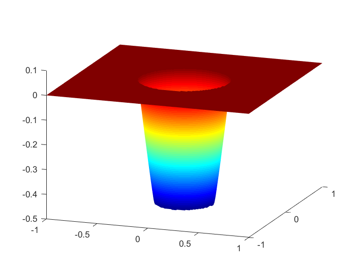
Remark 5.2.

Notice that we use the piecewise straight line $\Gamma_{h}$ as the interface instead of $\Gamma$ in this numerical example. The approximation is more and more accurate when refine the mesh.

Example 3. Compare with IFEM We also compare Nistche-XFEM with IFEM for the optimal control problem with interface. Consider the following example, interface $\Gamma$ is a circle, centered at $(0,0)$ with radius $r=\frac{1}{2}$ . $\Omega$ is a domain $[-1,1]\times[-1,1]$ .

\Omega_{1}=\{(x_{1},x_{2}):x_{1}^{2}+x_{2}^{2}\leq r^{2}\},\quad\Omega_{2}=\{(x_{1},x_{2}):x_{1}^{2}+x_{2}^{2}>r^{2}\}\cap\Omega.

We choose stable parameter $\lambda=10000h^{-1}$ , $\alpha_{1}=1,$ $\alpha_{2}=10$ , regulation parameter $a=0.01$ , and $U_{ad}=L^{2}(\Omega)$ .

\displaystyle u(x_{1},x_{2})=\begin{cases}\frac{5(x_{1}^{2}+x_{2}^{2}-r^{2})(x_{1}^{2}-1)(x_{2}^{2}-1)}{\alpha_{1}},&\mbox{ in $\Omega_{1}$ }\\ \frac{5(x_{1}^{2}+x_{2}^{2}-r^{2})(x_{1}^{2}-1)(x_{2}^{2}-1)}{\alpha_{2}},&\mbox{ in $\Omega_{2}$ }\end{cases}

(5.9)

\displaystyle y(x_{1},x_{2})=\begin{cases}\frac{(x_{1}^{2}+x_{2}^{2})^{\frac{3}{2}}}{\alpha_{1}},&\mbox{ in $\Omega_{1}$ }\\ \frac{(x_{1}^{2}+x_{2}^{2})^{\frac{3}{2}}}{\alpha_{2}}+(\frac{1}{\alpha_{1}}-\frac{1}{\alpha_{2}})r^{3},&\mbox{ in $\Omega_{2}$ }\end{cases}

(5.10)

\displaystyle p(x_{1},x_{2})=-au(x_{1},x_{2}).

(5.11)

N	$\\|u-u_{h}\\|_{0}$	order	$\\|y-y_{h}\\|_{0}$	order	$\\|p-p_{h}\\|_{0}$	order
16	1.1316e-02		4.4535e-03		1.1316e-04
32	3.0688e-03	1.88	1.1883e-03	1.91	3.0688e-05	1.88
64	7.5979e-04	2.01	3.1686e-04	1.91	7.5979e-06	2.01
128	1.8516e-04	2.04	7.6393e-05	2.05	1.8516e-06	2.04
256	4.2966e-05	2.11	1.8584e-05	2.04	4.2966e-07	2.11

Table 5:

L^{2}

errors of Nitsche-XFEM for Example 3.

N	$\|u-u_{h}\|_{1}$	order	$\|y-y_{h}\|_{1}$	order	$\|p-p_{h}\|_{1}$	order
16	1.1407e-01		1.1311e-01		1.1401e-03
32	5.7015e-02	1.00	5.8796e-02	0.94	5.6926e-04	1.00
64	2.7869e-02	1.03	2.9448e-02	1.00	2.7932e-04	1.03
128	1.3830e-02	1.01	1.4800e-02	0.99	1.3852e-04	1.01
256	6.8465e-03	1.01	7.3659e-03	1.00	6.8465e-05	1.01

Table 6:

H^{1}

errors of Nitsche-XFEM for Example 3.

N	$\\|u-u_{h}\\|_{0}$	order	$\\|y-y_{h}\\|_{0}$	order	$\\|p-p_{h}\\|_{0}$	order
16	1.1889e-02		4.6400e-03		1.1889e-04
32	3.1406e-03	1.92	1.2288e-03	1.91	3.1406e-05	1.92
64	7.0663e-04	2.15	3.1438e-04	1.96	7.0663e-06	2.15
128	1.6334e-04	2.11	8.1934e-05	1.93	1.6334e-06	2.11
256	3.5894e-05	2.18	2.1650e-05	1.92	3.5894e-07	2.18

Table 7:

L^{2}

errors of IFEM for Example 3. (From [67])

N	$\|u-u_{h}\|_{1}$	order	$\|y-y_{h}\|_{1}$	order	$\|p-p_{h}\|_{1}$	order
16	1.0665e-01		1.0778e-01		1.0665e-03
32	5.2602e-02	1.01	5.5660e-02	0.95	5.2602e-04	1.01
64	2.7054e-02	0.95	2.9084e-02	0.93	2.7054e-04	0.95
128	1.4028e-02	0.94	1.5047e-02	0.95	1.4028e-04	0.94
256	7.4170e-03	0.91	7.9081e-03	0.92	7.4170e-05	0.91

Table 8:

H^{1}

errors of IFEM for Example 3. (From [67])

In this example, the convergence order of Nitsche-XFEM is always full when the mesh is fine enough, our other numerical examples also show the fact. While for IFEM, the convergence order of $H^{1}$ semi-norm reduced from 1.01 to 0.91 when the mesh is refined.

6 Implementation aspects

In this section, we provide some details in our numerical experiments. If there is no constraint on the control i.e. $U_{ad}=L^{2}(\Omega)$ . We solve the optimal control problem with state equation (5.1), by solve the following linear system.

		$\displaystyle a_{h}(y_{h},v_{h})=l_{h}(v_{h})+(f,v_{h}),\quad\forall v_{h}\in V_{h}.$		(6.1)
		$\displaystyle a_{h}(p_{h},v_{h})=(y_{h}-y_{d},v_{h}),\quad\forall v_{h}\in V_{h}.$		(6.2)
		$\displaystyle p_{h}=-au_{h},$		(6.3)
		$\displaystyle y_{h}=b_{h},\ p_{h}=0,\quad on\ \partial\Omega.$		(6.4)

Where $b_{h}$ is the discrete boundary condition.

In order to illustrate how to solve the linear system, let us introduce some notations about the matrix and vector. The basis function of Nitsche-XFEM denote by $\phi_{i}$ .

		$\displaystyle A(i,j)=a_{h}(\phi_{i},\phi_{j}),$
		$\displaystyle M(i,j)=(\phi_{i},\phi_{j}),$
		$\displaystyle F_{1}(j)=(k_{2}g,\phi_{j,1})_{\Gamma_{h}}+(k_{1}g,\phi_{j,2})_{\Gamma_{h}}+(f,\phi_{j}),$
		$\displaystyle F_{2}(j)=-(y_{d},\phi_{j}).$

Where $i,j=1,2,3...,S$ , $S$ is the number of total degree of freedoms, $A$ is the stiffness matrix, $M$ is the mass matrix, $F_{1}$ and $F_{2}$ are column vectors. $(U_{h},Y_{h},P_{h})$ are column vectors consisting of corresponding degree of freedoms $(u_{h},y_{h},p_{h})$ . With these notations, the linear system (6.1)-(6.4) rewritten to,

	$\displaystyle AY_{h}$	$\displaystyle=MU_{h}+F_{1},$
	$\displaystyle AP_{h}$	$\displaystyle=MY_{h}+F_{2},$
	$\displaystyle P_{h}$	$\displaystyle=-aU_{h}.$

In matrix form,

$\begin{bmatrix}-aM&\textbf{0}&-M\\ \textbf{0}&-M&A\\ -M&A&\textbf{0}\end{bmatrix}$ $\begin{bmatrix}U_{h}\\ Y_{h}\\ P_{h}\end{bmatrix}$ $=\begin{bmatrix}\textbf{0}\\ F_{2}\\ F_{1}\end{bmatrix}$ .

The last is to apply boundary condition (6.4) to this system and solve it. Note we have to use special numerical integration scheme to get the stiffness matrix and mass matrix, because $\alpha$ and some basis functions are discontinuous across the interface. We simple divided the interface element into several sub-triangles and integrate these discontinuous functions on sub-triangles, see Fig. 6.

If $u$ is constrained, for example $U_{ad}=\{u\in L^{2}(\Omega):-\frac{1}{2}\leq u\leq\frac{1}{2}\ \text{a.e. in}\ \Omega\}$ . Then we can not use the above algorithm to solve the optimal control problem. The system became to a non-linear and non-smooth system.

		$\displaystyle a_{h}(y_{h},v_{h})=l_{h}(v_{h})+(f,v_{h}),\quad\forall v_{h}\in V_{h},$		(6.5)
		$\displaystyle a_{h}(p_{h},v_{h})=(y_{h}-y_{d},v_{h}),\quad\forall v_{h}\in V_{h},$		(6.6)
		$\displaystyle u_{h}=\min\left\{\frac{1}{2},\max\left\{-\frac{1}{2},-\frac{p_{h}}{a}\right\}\right\},$		(6.7)
		$\displaystyle y_{h}=b_{h},\ \ p_{h}=0,\quad\text{on}\ \partial\Omega.$		(6.8)

Because for any $p_{h}\in V_{h}$ , $u_{h}=\min\left\{\frac{1}{2},\max\left\{-\frac{1}{2},-\frac{p_{h}}{a}\right\}\right\}$ may not in $V_{h}$ . It makes the system difficult (or expensive) to solve in some cases, for example it is expensive when use high order finite element method to solve the system [56]. While the solution of Nitsche-XFEM is piecewise linear, we can easily apply fixed-point iteration or semi-smooth newton method [32] to solve the above system (6.5)-(6.8). We give a description of fixed-point iteration.

Algorithm

1.

Initialize $u^{i}_{h}=u^{0}$ ;
2.

Compute $y^{i}_{h}\in V_{h}$ by $a_{h}(y_{h}^{i},w_{h})=l^{i}_{h}(v_{h}),\forall v_{h}\in V_{h}$ ;
3.

Compute $p_{h}^{i}\in V_{h}$ by $a_{h}(v_{h},p_{h}^{i})=(y_{h}^{i}-y_{d},v_{h}),\forall v_{h}\in V_{h}$ ;
4.

Set $u_{h}^{i+1}=\max\{u_{a},\min\{-\frac{p_{h}}{a},u_{b}\}\}$ ;
5.

if $|u_{h}^{i+1}-u_{h}^{i}|<\text{Tol}$ or $i+1>\text{MaxIte}$ , then output $u_{h}=u_{h}^{i+1}$ , else $i=i+1$ , and go back to Step 2.

Where $u^{0}$ is an initial value, Tol is the tolerance, MaxIte is the maximal iteration number and $l^{i}_{h}(v_{h})=(u_{h}^{i},v_{h})+(f,v_{h})+(k_{2}g,v_{1,h})_{\Gamma_{h}}+(k_{1}g,v_{2,h})_{\Gamma_{h}}$ . This algorithm is convergent when the regularity parameter a is large enough (cf. [30]). If the regularity parameter $a$ is small, we recommend semi-smooth newton method.

In step 2, we also need special numerical integration scheme when computing $(u_{h}^{i},v_{h})$ . Because $u_{h}^{i}\in U_{ad}$ has constraints, see Fig. 7. It should be noticed that the numerical integration mesh is used only for the numerical integration.

7 Conclusion

In this paper, a numerical method has developed for optimal control problem govern by elliptic PDEs with interfaces. Optimal error estimations are derived for the state, co-state and control in an unfitted mesh. Our method is suitable for the model with non-homogeneous interface condition. Numerical results show our method is more stable for some problems compare with IFEM, stable means the convergence order do not reduce, when refine the mesh. There are many different XFEMs for different problems, but they are not used to solve the optimal control problem. We want to consider other XFEM for other optimal control problem, for example, XFEM for optimal control problem govern by elliptic PDEs in a non-convex domain.

References

[1] R. A. Adams. Sobolev spaces academic press. 1975.
[2] I. Babus̆ka and U. Banerjee. Stable generalized finite element method (sgfem). Computer Methods in Applied Mechanics and Engineering, 201-204(1):91–111, 2012.
[3] I Babus̆ka and J. M Melenk. The partition of unity method. International Journal for Numerical Methods in Engineering, 40(4):727–758, 2015.
[4] Ivo Babus̆ka. The finite element method for elliptic equations with discontinuous coefficients. Computing, 5(3):207–213, 1970.
[5] Ivo Babus̆ka, Gabriel Caloz, and John E. Osborn. Special finite element methods for a class of second order elliptic problems with rough coefficients. Siam Journal on Numerical Analysis, 31(4):945–981, 1994.
[6] Nelly Barrau, Roland Becker, Eric Dubach, and Robert Luce. A robust variant of nxfem for the interface problem. Comptes Rendus Mathematique, 350(15-16):789–792, 2012.
[7] J.W. Barrett and C.M. Elliott. Fitted and unfitted finite-element methods for elliptic equations with smooth interfaces. IMA J. Numer. Anal., 7(3):283–300, 1987.
[8] R. Becker, H. Kapp, and R. Rannacher. Adaptive finite element methods for optimal control of partial differential equations: Basic concept. SIAM J. Control Optim., 39(1):113–132, 2000.
[9] Roland Becker, Erik Burman, and Peter Hansbo. A nitsche extended finite element method for incompressible elasticity with discontinuous modulus of elasticity. Computer Methods in Applied Mechanics and Engineering, 198(41-44):3352–3360, 2009.
[10] Ted Belytschko, Robert Gracie, and Giulio Ventura. A review of extended/generalized finite element methods for material modeling. Modelling Simulation in Materials Science Engineering, 17:043001, 2009.
[11] O. Benedix and B. Vexler. A posteriori error estimation and adaptivity for elliptic optimal control problems with state constraints. Comput. Optim. Appl., 44(1):3–25, 2009.
[12] J.H. Bramble and J.T. King. A finite element method for interface problems in domains with smooth boundaries and interfaces. Adv. Comput. Math., 6(1):109–138, 1996.
[13] E. Burman, S. Claus, P. Hansbo, M.G. Larson, and A. Massing. Cutfem: Discretizing geometry and partial differential equations. Int. J. Numer. Meth. Engng, 104(7):472–501, 2015.
[14] Z. Cai, C. He, and S. Zhang. Discontinuous finite element methods for interface problems: Robust a priori and a posteriori error estimates. SIAM J. Numer. Anal., 55(1):400–418, 2017.
[15] B. Camp, T. Lin, Y. Lin, and W. Sun. Quadratic immersed finite element spaces and their approximation capabilities. Adv. Comput. Math., 24(1-4):81–112, 2006.
[16] E. Casas. Control of an elliptic problem with pointwise state constraints. SIAM J. Control Optim., 24(6):1309–1318, 1986.
[17] M. Cenanovia, P. Hansbo, and M.G. Larson. Cut finite element modeling of linear membranes. Comput. Methods Appl. Mech. Engrg., 310:98–111, 2016.
[18] Z. Chen and J. Zou. Finite element methods and their convergence for elliptic and parabolic interface problems. Numer. Math., 79(2):175–202, 1998.
[19] Kwok Wah Cheng and Thomas Peter Fries. Higher-order xfem for curved strong and weak discontinuities. International Journal for Numerical Methods in Engineering, 82(5):564–590, 2010.
[20] So Hsiang Chou, Do Y. Kwak, and K. T. Wee. Optimal convergence analysis of an immersed interface finite element method. Advances in Computational Mathematics, 33(2):149–168, 2010.
[21] R. S. Falk. Approximation of a class of optimal control problems with order of convergence estimates. J. Math. Anal. Appl., 44(1):28–47, 1973.
[22] R. Fedkiw. The immersed interface method. numerical solutions of pdes involving interfaces and irregular domains. Math. Comput., 76(259):1691, 2006.
[23] W. Gong and N. Yan. Adaptive finite element method for elliptic optimal control problems: convergence and optimality. Numer. Math., 135(4):1121–1170, 2017.
[24] Daoru Han, Pu Wang, Xiaoming He, Tao Lin, and Joseph Wang. A 3d immersed finite element method with non-homogeneous interface flux jump for applications in particle-in-cell simulations of plasma-lunar surface interactions. Journal of Computational Physics, 321:965–980, 2016.
[25] Anita Hansbo and Peter Hansbo. An unfitted finite element method, based on nitsches method, for elliptic interface problems. Computer Methods in Applied Mechanics and Engineering, 191(47-48):5537–5552, 2002.
[26] P. Hansbo, M.G. Larson, and S. Zahedi. A cut finite element method for a stokes interface problem. Appl. Numer. Math., 85(C):90–114, 2014.
[27] Xiaoming He, Tao Lin, and Yanping Lin. Immersed finite element methods for elliptic interface problems with non-homogeneous jump conditions. International Journal of Numerical Analysis Modeling, 8(2):284–301, 2011.
[28] M. Hintermüeller and R. H. W. Hoppe. Goal-oriented adaptivity in pointwise state constrained optimal control of partial differential equations. SIAM J. Control Optim., 48(8):5468–5487, 2010.
[29] M. Hinze. A variational discretization concept in control constrained optimization: the linear-quadratic case. Comput. Optim. Appl., 30(1):45–61, 2005.
[30] M. Hinze, R. Pinnau, M. Ulbrich, and S. Ulbrich. Optimization with PDE Constraints, volume 23. Springer, 2008.
[31] Michael Hinze and Morten Vierling. Variational discretization and semi-smooth newton methods; implementation, convergence and globalization in pde constrained optimization with control constraints. Immunogenetics, 55(7):429–436, 2009.
[32] Michael Hinze and Morten Vierling. A globalized semi-smooth newton method for variational discretization of control constrained elliptic optimal control problems. 2012.
[33] J. Huang and J. Zou. A mortar element method for elliptic problems with discontinuous coefficients. IMA J. Numer. Anal., 22(4):549–576, 2002.
[34] Kenan Kergrene, Ivo Babus̆ka, and Uday Banerjee. Stable generalized finite element method and associated iterative schemes; application to interface problems. Computer Methods in Applied Mechanics and Engineering, 305:1–36, 2016.
[35] K. Kohls, K. G. Siebert, and A. Rösch. Convergence of adaptive finite elements for optimal control problems with control constraints. In Leugering G. et al., editor, Trends in PDE Constrained Optimization. 2014.
[36] Christoph Lehrenfeld. The nitsche xfem-dg space-time method and its implementation in three space dimensions. Siam Journal on Scientific Computing, 37(1):A245–A270, 2014.
[37] Christoph Lehrenfeld and Arnold Reusken. Analysis of a dg-xfem discretization for a class of two-phase mass transport problems. Siam Journal on Numerical Analysis, 52(52):958–983, 2012.
[38] Christoph Lehrenfeld and Arnold Reusken. Optimal preconditioners for nitsche-xfem discretizations of interface problems. Numerische Mathematik, 135(2):1–20, 2014.
[39] J. Li, M.J. Markus, B. Wohlmuth, and J. Zou. Optimal a priori estimates for higher order finite elements for elliptic interface problems. Appl. Numer. Math., 60(1-2):19–37, 2010.
[40] R. Li, W.B. Liu, H.P. Ma, and Tang T. Adaptive finite element approximation for distributed elliptic optimal control problems. SIAM J. Control Optim., 41(5):1321–1349, 2002.
[41] Z. Li and K. Ito. The immersed interface method: numerical solutions of PDEs involving interfaces and irregular domains. Frontiers Appl. Math. 33. SIAM, Philadelphia, 2006.
[42] Z. Li, T. Lin, and X. Wu. New cartesian grid methods for interface problems using the finite element formulation. Numer. Math., 96(1):61–98, 2003.
[43] T. Lin, Y. Lin, and W. Sun. Error estimation of a class of quadratic immersed finite element methods for elliptic interface problems. Discrete Contin. Dyn. Syst. Ser. B, 7(4):807–823, 2007.
[44] T. Lin, Y. Lin, and X. Zhang. Partially penalized immersed finite element methods for elliptic interface problems. SIAM J. Numer. Anal., 53(2):1121–1144, 2015.
[45] Tao Lin, Qing Yang, and Xu Zhang. Partially penalized immersed finite element methods for parabolic interface problems. Numerical Methods for Partial Differential Equations, 31(6):1925–1947, 2015.
[46] W. Liu, W. Gong, and N. Yan. A new finite element approximation of a state-constained optimal control problem. J. Comput. Math., 27(1):97–114, 2009.
[47] Nicolas Moes, John E Dolbow, and Ted Belytschko. A finite element method for crack growth without remeshing. International Journal for Numerical Methods in Engineering, 46(1):131–150, 1999.
[48] Serge Nicaise, Yves Renard, and Elie Chahine. Optimal convergence analysis for the extended finite element method. International Journal for Numerical Methods in Engineering, 86(4-5):528–548, 2011.
[49] J. Nitsche. Über ein variationsprinzip zur lösung von dirichlet-problemen bei verwendungvon von teilräumen, die keinen randbedingungen unterworfen sind. Abh. Math. Univ. Hamburg, 36(1):9–15, 1971.
[50] M. Plum and C. Wieners. Optimal a priori estimates for interface problems. Numer. Math., 95(4):735–759, 2003.
[51] Schneider R and Wachsmuth G. A posteriori error estimation for control-constrained, linear-quadratic optimal control problems. SIAM J. Numer. Anal., 54(2):1169–1192, 2016.
[52] A. Rösch, K.G. Siebert, and S. Steinig. Reliable a posteriori error estimation for state-constrained optimal control. Comput. Optim. Appl., 68(1):121–162, 2017.
[53] A. Rösch and S. Steinig. A priori error estimates for a state-constrained elliptic optimal control problem. ESAIM Math. Model. Numer. Anal., 46(5):1107–1120, 2012.
[54] A. Rösch and D. Wachsmuth. A-posteriori error estimates for optimal control problems with state and control constraints. Numer. Math., 120(4):733–762, 2012.
[55] B. Schott. Stabilized cut finite element methods for complex interface coupled flow problems. PhD thesis, Technische Universität München, 2017.
[56] David Sevilla and Daniel Wachsmuth. Polynomial integration on regions defined by a triangle and a conic. In International Symposium on Symbolic and Algebraic Computation, pages 163–170, 2010.
[57] Soheil Soghrati, Alejandro M Aragón, C Armando Duarte, and Philippe H Geubelle. An interface-enriched generalized fem for problems with discontinuous gradient fields. International Journal for Numerical Methods in Engineering, 89(8):991–1008, 2012.
[58] Soheil Soghrati and Philippe H. Geubelle. A 3d interface-enriched generalized finite element method for weakly discontinuous problems with complex internal geometries. Computer Methods in Applied Mechanics and Engineering, 217-220(1):46–57, 2012.
[59] T. Strouboulis, I. Babus̆ka, and K. Copps. The design and analysis of the generalized finite element method. Computer Methods in Applied Mechanics and Engineering, 181(1):43–69, 2000.
[60] Theofanis Strouboulis, Ivo Babus̆ka, and Realino Hidajat. The generalized finite element method for helmholtz equation: Theory, computation, and open problems. Computer Methods in Applied Mechanics Engineering, 195(37-40):4711–4731, 2006.
[61] D. Tiba and F. Tröltzsch. Error estimates for the discretization of state constrained convex control problems. Numer. Funct. Anal. Optim., 17(9-10):1005–1028, 1996.
[62] Fredi Tröltzsch. Optimal control of partial differential equations: Theory, methods and applications. Siam Journal on Control Optimization, 112(2):399, 2010.
[63] Fei Wang, Yuanming Xiao, and Jinchao Xu. High-order extended finite element methods for solving interface problems. 2016.
[64] J. Xu and S. Zhang. Optimal finite element methods for interface problems. In T. Dickopf et al., editor, Domain Decomposition Methods in Science and Engineering XXII, volume 104 of Lecture Notes in Computational Science and Engineering, pages 77–91. Springer, Cham, 2016.
[65] Jin Chao Xu. Estimate of the convergence rate of the finite element solutions to elliptic equation of second order with discontinuous coefficients. Natural Science Journal of Xiangtan University, 1982.
[66] Yan, Gong, Zhilin, Li, Department, and Gaffney. Immersed interface finite element methods for elasticity interface problems with non-homogeneous jump conditions. Numerical Mathematics Theory Methods Applications, 46(1):472–495, 2007.
[67] Qian Zhang, Kazufumi Ito, Zhilin Li, and Zhiyue Zhang. Immersed finite elements for optimal control problems of elliptic pdes with interfaces. Journal of Computational Physics, 298(C):305–319, 2015.

	$\displaystyle\|v_{h}(x)\|^{2}$	$\displaystyle=\left\|\sum^{n-1}_{i=0}(v_{h}(x_{i+1})-v_{h}(x_{i}))\right\|^{2}$
		$\displaystyle=\left\|\sum^{n-1}_{i=0}\nabla{v_{h}(\bar{x})(x_{i+1}-x_{i})}\right\|^{2}$
		$\displaystyle\leq n\sum^{n-1}_{i=0}\|\nabla{v_{h}(\bar{x}_{i})}\|^{2}h_{i}^{2}$
		$\displaystyle\lesssim n\sum^{n-1}_{i=0}\|\nabla v_{h}\|^{2}_{0,T_{i}}.$

	$\displaystyle nh^{2}\sum^{n-1}_{i=0}\|\nabla v_{h}\|^{2}_{0,T_{i}}$	$\displaystyle\lesssim h\sum^{n-1}_{i=0}\|\nabla v_{h}\|^{2}_{0,T_{i}}$
	$\displaystyle\int_{T}\|v_{h}\|^{2}ds$	$\displaystyle\lesssim h\sum^{n-1}_{i=0}\|\nabla v_{h}\|^{2}_{0,T_{i}}.$

	$\displaystyle\|\|p_{h}-p^{h}\|\|^{2}_{0}$	$\displaystyle\lesssim\|\|\|p_{h}-p^{h}\|\|\|^{2}$
		$\displaystyle\lesssim a_{h}(p_{h}-p^{h},p_{h}-p^{h})=(y_{h}-y,p_{h}-p^{h})$
		$\displaystyle\lesssim\|\|y_{h}-y\|\|_{0}\|\|p_{h}-p^{h}\|\|_{0}.$

	$\displaystyle\|\|\|y_{h}-y^{h}\|\|\|^{2}$	$\displaystyle\lesssim a_{h}(y_{h}-y^{h},y_{h}-y^{h})=(u_{h}-u,y_{h}-y^{h})$
		$\displaystyle\leq\\|u-u_{h}\\|_{0}\\|y-y^{h}\\|_{0}$
		$\displaystyle\lesssim\\|u-u_{h}\\|_{0}\|\|\|y_{h}-y^{h}\|\|\|.$

	$\displaystyle\|\|\|p_{h}-p^{h}\|\|\|^{2}$	$\displaystyle\lesssim a_{h}(p_{h}-p^{h},p_{h}-p^{h})=(y_{h}-y,p_{h}-p^{h})$
		$\displaystyle\lesssim\|\|y_{h}-y\|\|_{0}\|\|p_{h}-p^{h}\|\|_{0}$
		$\displaystyle\lesssim\|\|y_{h}-y\|\|_{0}\|\|\|p_{h}-p^{h}\|\|\|,$