Interpreting Electrical-Resistivity Tomography measurements using Neural Network
Abstract
Electrical Resistivity Tomography (ERT) has been extensively used for imaging the subsurface resistivity distribution and structure. Over the years, many algorithms have been developed in order to solve the subsurface resistivity distribution from the ERT measurements. In this paper a new method for interpreting the ERT measurements is presented. Using supervised learning to train a neural network, we are able to interpret the ERT measurement into a 2D image of the underground resistivity up to depths of 50 meters while using a simple Wenner-Schlumberger survey of 96 electrodes with 1 meter spacing. The neural network is trained and tested using simulative data and it is shown to have superior results over a well established inversion method.
Keywords:
Neural Networks; Electric Resistivity TomographyI Introduction
Electrical Resistivity Tomography (ERT) is a method which allows the imaging of the electrical conductivity profile of the ground in an unobtrusive manner [1]. A typical survey, as investigated in this work, is conducted by placing electrodes in a linear formation, with some spacing between the electrodes. Measurements are performed by applying a near steady-state current (up to a few amperes) between two electrodes and measuring the voltage between two other electrodes. This procedure is carried out using all the relevant electrodes for the survey [2].
Due to the fact that the current flows in an unknown path which is determined by the conductivity profile of the ground, the interpretation is not straightforward. Moreover, the number of unknown in the problem is larger than the number of equations; therefore this problem is ill-posed and needs to be solved using iterative inversion methods [3, 4]. The inversion process begins with an initial (hopefully intelligent) guess of the under-surface resistivity and the forward simulated measurements on this guessed profile. At each iteration the resistivity profile is changed in a certain way in order to minimize some cost function (which includes the difference between the simulated forward solutions and the actual measurements and some other constrains) [5, 6]. However, the final solution is sensitive to both the initial guess and the choice of constrains and cost function. In order to overcome those difficulties in interpreting the ERT measurements, providing a 2D imaging of the subsurface resistivity profile, this paper introduces a different approach based on supervised learning for training a Neural Network (NN).
In the past few years there have been a major advancement in training and implementing neural networks (NN) in many different fields. Nowadays, (deep) Neural Networks are the state-of-the-art in many classification and prediction tasks. NN are now able to translate sentences [7], generate new art [8] and even define communication protocol [9]. The idea of using a NN for interpretation of the under-surface geophysical properties is not new and has been suggested almost three decades ago [10]. During recent years NN have been applied to analyzing gravity measurments [11], seismic waveform inversion [12], data from ground penetrating radar [13] and more.
A prior work was performed by [14] which demonstrated the ability to interpret geophysical measurements by artificial neural networks. The assumption of the solution was of a layered ground profile and the solution determined the depths and resistivities of 5-6 layers. In our case the output is a full 2D image without the need to define, a-priori, a sub-surface model. Another major difference is the scales, where in [14] the survey had hundreds of meters of electrode separation and the depths of interpretation were 1 km, trading off resolution. However, we aim our work at shallow ERT and high resolution of .
The rest of this manuscript is organized as follows. The definition of the ground resistivity profile and details about modelling the ERT survey are given in section II. Section III deals with the description of the NN and the database we used for training it. The results of the NN and a comparison to a widely used inversion program are shown in section IV and concluding remarks are given at section V.
II Model and Simulations
The subsurface structure is (in general) inhomogeneous thus, in order to increase the validity of the presented method, we have simulated inhomogeneous ground by assuming random resistivity values with spatial correlations. The simulated underground structure is a matrix where each element, , represents the resistivity of a cross section at horizontal position and depth . The ground resistivity profile is a linear gradient perturbed by random Gaussian
| (1) |
where is measured in meters, is a Gaussian centred at with width. The values of are taken from uniform distributions and , respectively. The center of the Gaussians, are random variables uniformly distributed in the underground. A typical simulated ground is depicted in Figure 1.

There are several well-known survey protocols that are commonly used today. The main differences between the protocols are: (i) the depth of investigation, (ii) the sensitivity of the array to vertical and horizontal changes in the subsurface resistivity, (iii) the horizontal data coverage and (iv) the signal strength [15]. Since the ground model we used in the simulations have changes of resistivity values in both horizontal and vertical directions, we have decided to use the “Wenner-Schlumberger” (WS) survey method. The main advantage of the WS array is its sensitivity to both vertical and horizontal changes.
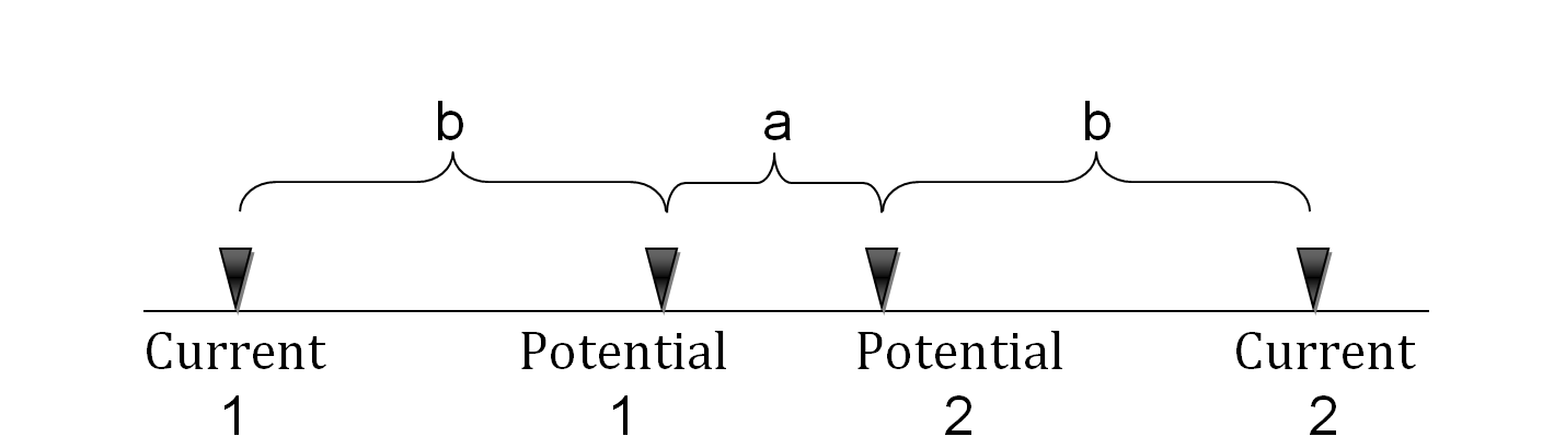
The WS array is defined by three parameters: which is the distance between the inner potential electrodes and which defines the distance between a potential electrode to the closest current electrode in terms of multiplication of as shown in Fig. 2. A third parameter of the array is the location of the left current electrode (current 1 in fig. 2). In order to maintain a reasonable number of measurements, we used and and for each value of the pair we used all possible position for the current 1 electrode. As a result, this protocol contained 1488 measurements of the apparent resistivity. The forward simulation of the ERT measurements was carried out using R2 software [16] and the simulated ground has been extended far away to minimize boundary effects on the results.
III Neural Network
When trying to interpret the measurements of an ERT survey (as in any inversion problem) one asks the question what is the medium which caused the acquired measurements. Thus, if we have enough examples of the medium and the out-coming ERT measurements we can try and get insights about the inverse relation between the measurements and the medium which caused them. This approach, for training a neural network is called ”supervised learning”.
We have simulated a massive database of examples - random grounds as defined by (1) and a forward modelling of the 1488 ERT measurements has been carried out for each ground. The database thus consisted of pairs - the ground matrix and the resulting ERT measurements vector, respectively. We have randomly split the dataset into a training set consisting of approximately of the examples and the remaining examples were used to test the training of the neural network.
The input of the neural network is the ERT measurements vector which consist of 1488 measurements and the output is a ground matrix with dimensions . In order to have as simple solution as possible, we used only one hidden layer of 250 neurons with a activation function
| (2) |
The overall model is given by
| (3) |
where bold letters stand for vectors. are the weight matrices of the corresponding layers and are the corresponding bias vectors. The output vector is reshaped into a matrix which is the ground predicted by the neural network model.
In order to train the NN, a loss (a.k.a. cost) function must be defined. In many application one uses the euclidean distance between the prediction and ground truth . However, in this scenario it turned out that an loss function
| (4) |
results in a better performance and shorter convergence time.
The weights and biases were initializes to be normally distributed with standard deviation of and we used the Adam optimizer to train the NN. Each batch consisted of 50 examples pairs of ground and ERT measurements and the network has been trained for 1000 epochs.
IV Results and comparison

![[Uncaptioned image]](1805.03698v1/examples_wrt_nn.png) |
![[Uncaptioned image]](1805.03698v1/examples_wrt_r2.png) |
The usual way to examine the results of an inversion process is by comparing the ERT measurements obtained from the forward solution of the true ground to the ERT measurements of the predicted ground and calculating some loss function . When the loss function is small enough the inversion process stops. However, this does not guaranty that the predicted ground is similar to the true ground . In the scenario of real measurements in the field, this is the best one can do with an inversion process. However, using simulated data we can make a comparison between the real goal of the inversion process - the predicted ground and the true ground .
In order to compare the results of the NN to the classical inversion method we used R2 program to predict the grounds for the 1500 test examples. The parameters we used for the inversion process were: background resistivity of , tolerance of , maximum of 10 iterations 11 1 For more detail about the meaning of each parameter, please refere to the R2 manual [16]. The requested output from the inversion has the same size and resolution as the NN predictions and the true grounds: width of and depth of with resolution of .
The comparison between the NN prediction and the predictions of the inversion process is done by using two parameters. The first one is the loss (4) of each prediction made by NN and R2. It is also interesting to have a measure of the overall similarity of values between the prediction and the true ground. This can be done by using the same distance between the histogram of the predicted ground and the histogram of the true ground. This way, slightly spatially shifted features will not cause large penalty.
Figure 3 depicts the histograms of the loss for the predictions made by both the NN and R2. It is very clear that while R2 have a very large span of errors, ranging from 50 to 150, the NN achieves errors of around 50 in its worst case. While Loss is very sensitive to the value of each pixel in the ground, the Loss of the histogram is a comparison of the distributions. Comparing the values of for both histograms with respect to the true ground (right panel of Fig. 3) we find that the NN have a narrow distribution of Loss values and the values are closer to 0 than the Loss of the predictions made by R2.
An illustration of the different sub-surface reconstruction is shown in Table 1. Within each column of 3 images, the middle panel is the true ground, the upper panel is the prediction of the neural network and the lower panel is the prediction of the inversion process using R2. It is clear that in all the examples the NN has a better performance than the classical inversion method.
V Conclusions
We have demonstrate the ability to reconstruct the sub-surface resistivity profile from an ERT survey using a trained neural network. As shown in Figure 3, the predictions using neural network are more accurate than the ground predicted by using the traditional inversion method. Moreover, the neural network is capable of predicting the underground resistivity structure even at depth of 40-50 meters which are well beyond the maximal depth of the described inversion method. Although the mapping at those depths is not perfect, the main features are visible and recognizable and in many practical cases a slight deformation or offset is within the tolerance of acceptable solutions. Another feature of the neural network is that the prediction process is obviously faster than conventional inversion algorithms and results are produced within milliseconds of receiving the ERT measurements from the field. Future research will include the extension of this approach for using other survey protocols, reducing the number of measurements in the survey and taking into account the effect of various noises on the performance of the neural network predictions.
References
- [1] G. Morelli and D. J. LaBrecque, European Journal of Environmental and Engineering Geophysics 1, 171 (1996).
- [2] R. Saad, M. Nawawi, and E. Mohamad, Electronic Journal of Geotechnical Engineering 17, 369 (2012).
- [3] P. Tsourlos and R. Ogilvy, Journal of the Balkan Geophysical Society 2, 30 (1999).
- [4] M. Camporese, G. Cassiani, R. Deiana, P. Salandin, and A. Binley, Water Resources Research 51, 3277 (2015), ISSN 1944-7973, URL http://dx.doi.org/10.1002/2014WR016017.
- [5] J. Vanderborght, A. Kemna, H. Hardelauf, and H. Vereecken, Water Resources Research 41, n/a (2005), ISSN 1944-7973, w06013, URL http://dx.doi.org/10.1029/2004WR003774.
- [6] M. Loke, T. Dahlin, and D. Rucker (2014).
- [7] Y. Wu, M. Schuster, Z. Chen, Q. V. Le, M. Norouzi, W. Macherey, M. Krikun, Y. Cao, Q. Gao, K. Macherey, et al., CoRR abs/1609.08144 (2016), eprint 1609.08144, URL http://arxiv.org/abs/1609.08144.
- [8] J.-Y. Zhu, T. Park, P. Isola, and A. A. Efros, arXiv preprint arXiv:1703.10593 (2017).
- [9] O. Naparstek and K. Cohen, CoRR abs/1704.02613 (2017), eprint 1704.02613, URL http://arxiv.org/abs/1704.02613.
- [10] A. Raiche, Geophys. J. Int. 105, 629 (1991).
- [11] P. S. Alireza HAJIAN, Hossein ZOMORRODIAN, Acta Geophysica 60, 1043 (2012).
- [12] S. Yuan, J. Liu, S. Wang, T. Wang, and P. Shi, IEEE Geoscience and Remote Sensing Letters 15, 272 (2018), ISSN 1545-598X.
- [13] B. Ehret, Geoderma 160, 111 (2010).
- [14] S. Upendra K.Singh, R.K.Tiwari, Computers & Geosciences 52, 246 (2013).
- [15] M. Loke, Geotomo Software, Malaysia (2006), URL http://www.geotomosoft.com/coursenotes.zip.
- [16] A. Binley, R2 version 3.1 june 2016, URL http://www.es.lancs.ac.uk/people/amb/Freeware/R2/R2.htm.