跳到论文正文
W Papers独立论文阅读器 arXiv:1805.03477 论文正文 计算阅读时间 · 0%
引用这篇论文根据当前论文元数据生成,正式投稿前建议核对。


License: arXiv.org perpetual non-exclusive license
arXiv:1805.03477v3 [quant-ph] 11 Mar 2019

Optimal universal learning machines for quantum state discrimination

Marco Fanizza    Andrea Mari    Vittorio Giovannetti ††thanks: Marco Fanizza is with NEST, Scuola Normale Superiore, Istituto Nanoscienze-CNR, I-56126 Pisa, Italy.††thanks: Andrea Mari is with NEST, Scuola Normale Superiore, Istituto Nanoscienze-CNR, I-56126 Pisa, Italy. Now at Xanadu, 777 Bay Street, Toronto, Ontario, M5G 1S5, Canada. ††thanks: Vittorio Giovannetti is with NEST, Scuola Normale Superiore and Istituto Nanoscienze-CNR, I-56126 Pisa, Italy.
Abstract

We consider the problem of correctly classifying a given quantum two-level system (qubit) which is known to be in one of two equally probable quantum states. We assume that this task should be performed by a quantum machine which does not have at its disposal a complete classical description of the two template states, but can only have partial prior information about their level of purity and mutual overlap. Moreover, similarly to the classical supervised learning paradigm, we assume that the machine can be trained by nn qubits prepared in the first template state and by nn more qubits prepared in the second template state. In this situation we are interested in the optimal process which correctly classifies the input qubit with the largest probability allowed by quantum mechanics. The problem is studied in its full generality for a number of different prior information scenarios and for an arbitrary size nn of the training data. Finite size corrections around the asymptotic limit n→∞n\rightarrow\infty are derived. When the states are assumed to be pure, with known overlap, the problem is also solved in the case of d-level systems.

I Introduction

Machine Learning (ML) is that branch of computer science which studies how to instruct a computer to solve a specific task by feeding it with a collection of training data from which it could learn how to proceed. This approach finds applications in a variety of practical pattern recognition, decision and clustering problems where a definite classification of the various alternatives are not directly accessible [1]. Not surprisingly, the interplay between ML and quantum information is very promising (see [2], [3], [4], [5], [6] and references therein). ML has been proposed as a useful tool to improve the performances of a variety of quantum information procedures, e.g. identification of optimal quantum measurement and estimation procedures, quantum gate design and quantum dynamics engineering. On the other hand, it has been shown that quantum computing can provide speed-ups for ML problems. Moreover, as originally hinted in Refs. [8, 9, 10, 11, 12], a drastic departure from classical data analysis is instead realized in Quantum Learning (QL), where the “learning from examples” paradigm is adopted as a new mode of operation of quantum devices which have access to (not necessarily classical) training data. This setting appears to be perfectly suited to deal with the specific character of quantum mechanics where, at variance with classical models, a fundamental discrepancy exists between the state of a system and the “knowledge” one can acquire about it through measurements. Such discrepancy is a distintive feature of the theory: ultimately it can be traced back to the no-cloning theorem [16] and poses intrinsic limitations on information retrieval processes. Accordingly in quantum mechanics, the ability of perfectly discriminating alternative configurations, let them being states or processes, can only be guaranteed under special conditions (semiclassical limit). Since the seminal works of Helstrom [13], Holevo [14] and Yuen et al. [15], developing optimal probabilistic strategies to face these limitations is a fundamental problem of quantum information. A standard example is provided by quantum state discrimination: here an agent is presented with a quantum system QQ and asked to identify its state knowing that the latter was randomly drawn from an ensemble of possible alternatives which are specified in terms of classical data that fully characterize them. The QL version of this problem is obtained by replacing such classical descriptions with a collection of quantum ancillary systems initialized into the same template states the agent has to assign to QQ. A universal machine for optimal discrimination is hence identified as the quantum device which, by having full access to QQ and the ancillas, allows the agent to solve the identification task with the smallest probability of error. The problem has been addressed in various scenarios in [10, 11, 17, 18, 19, 23, 25, 24], and has attracted the attention of the community as an example of a genuine supervised QL task  [4, 5, 7]. In this article we present results about universal machines for qubit discrimination, which can discriminate among any two states, extending in particular the results of [19] to include a variety of scenarios. Specifically we focus on hybrid QL configurations where the agent, beside being provided with the quantum ancillas, has also access to some prior classical information on the templates configurations, such as their purity or their mutual distance. These scenarios naturally emerge when, for instance, the training and the target data are effected by some deteriorating processes (say dephasing or decoherence transformations) which the agent cannot prevent from occurring, but whose operating mechanisms are known to him, or when the different templates are affected by uncertainties arising from the absence of a common, shared reference frame.

The manuscript is organized as follows: notation and model are introduced in Sec. II. The principal part of the paper is Sec. III where our results are explicitly derived in three dedicated subsections. In the first two paragraphs we extend the results of the work of Ref. [19]. Specifically in Sec. III-A we study the case of an optimal universal machines which is trained to discriminate between two qubit density matrices of fixed but different purities. In Sec. III-B instead we focus on the case where the training data are two generic (possibly) mixed quantum systems. In Sec. III-C we discuss the scenario where the training data are pure with fixed relative overlap, but otherwise unknown. The interest in this last configuration arises when considering QML processes where, in analogy with the schemes analyzed in Refs. [26, 27, 28, 30, 29], the party who is creating the template states does not share a common reference frame with the party that is supposed to solve the identification problem. For this special setting results are extended beyond the qubit case to include arbitrary dd-dimensional input systems. Finally in Sec. III-D we compare the optimal machines that leads to the optimal probability thresholds for the three scenarios, commenting about their compatibility. Section IV presents an implementation of optimal machines obtained by exploiting the QISKit software development kit [35].

The paper ends with conclusions in Sec. V. Technical material is presented in dedicated appendices.

II The model

In a classical supervised learning classification problem an algorithm receives as input a training set of labelled data, and outputs a classifier which can be used to predict the label of new unlabelled data. In a probabilistic setting one can suppose that the dataset, made of couples (x,y)(x,y) of data x∈Xx\in X and labels y∈Yy\in Y obeys a probability distribution P:X×Y→[0,1]P:X\times Y\rightarrow[0,1]. Then, a classifier is a labelling rule obeying another probability distribution C:X→YC:X\rightarrow Y. For each PP there exists an optimal classifier which minimises the probability of misclassification; a good learning algorithm should obtain a classifier that with a misclassification probability close to the optimal, as the training dataset becomes large, and with the fewest assumptions on the distribution PP. The assumptions on PP can also be described probabilistically as a prior probability distribution GG over the possible PP. Given this prior GG, one can say that an algorithm is optimal if it attains the lowest probability on average, where the average is done over all the possible distributions PP, assuming they are distributed according to GG. A straightforward way to generalise classical probabilistic task is to substitute probability distributions with quantum states: in the problem considered in this article, we substitute conditional probabilities P⁡(X|Y)P(X|Y) with quantum states distributed according a classical prior. More precisely in the scenario we have in mind a qubit system XX is initialized with probability 1/21/2 in one of two possible template states ρ1\rho_{1} and ρ2\rho_{2}. Without having access to the full classical description of these templates configurations (i.e. without knowing the explicit values of their associated Bloch vectors 𝐫1\mathbf{r}_{1} and 𝐫2\mathbf{r}_{2}, see below), an external agent is now asked to identify which of the two alternative actually occurred by only granting him access to XX and to two independent sets of nn ancillary qubits AA and BB, initialized respectively into nn copies of ρ1\rho_{1} and ρ2\rho_{2}. Following Refs. [10, 11, 19, 23] solutions to this problem can be assigned in terms of a two-outcome POVM ℳ^≡{Π^1,Π^2}\hat{\mathcal{M}}\equiv\{\hat{\Pi}_{1},\hat{\Pi}_{2}\} that acts globally on the full system A​X​BAXB formed by the test qubit XX and by the two nn-qubits ancillas. In particular, noticing that the possible states of A​X​BAXB are the density matrices τ1=ρ1⊗n⊗ρ1⊗ρ2⊗n\tau_{1}=\rho_{1}^{\otimes n}\otimes\rho_{1}\otimes\rho_{2}^{\otimes n} (corresponding to have XX in ρ1\rho_{1}) and τ2=ρ1⊗n⊗ρ2⊗ρ2⊗n\tau_{2}=\rho_{1}^{\otimes n}\otimes\rho_{2}\otimes\rho_{2}^{\otimes n} (XX in ρ2\rho_{2}), the average error probability of the procedure can be computed as

Pe​r​r(n)=∫d​μ​(ρ1,ρ2)​Tr​[τ1​Π^2]+Tr​[τ2​Π^1]2,\displaystyle P_{err}^{(n)}=\int d\mu(\rho_{1},\rho_{2})\frac{\mbox{Tr}[\tau_{1}\hat{\Pi}_{2}]+\mbox{Tr}[\tau_{2}\hat{\Pi}_{1}]}{2}, (1)

where Tr​[τj​Π^j]\mbox{Tr}[\tau_{j}\hat{\Pi}_{j}] is the probability of success in the identifying the jj-th configuration, while d​μ​(ρ1,ρ2)d\mu(\rho_{1},\rho_{2}) is a probability measure that gauges the initial ignorance of the agent about ρ1\rho_{1} and ρ2\rho_{2}. Exploiting then the completeness relation of ℳ^\hat{\mathcal{M}} this can be finally recast into

Pe​r​r(n)=12−14​Tr​[Θ⁡(Π^1−Π^2)],\displaystyle P_{err}^{(n)}=\frac{1}{2}-\frac{1}{4}\mbox{Tr}[\Theta(\hat{\Pi}_{1}-\hat{\Pi}_{2})]\;, (2)

where Θ\Theta is the trace-null, Hermitian operator

Θ=α(n)−β(n),\displaystyle\Theta={\alpha^{(n)}}-{\beta^{(n)}}\;, (3)

given by the difference between the following density matrices of A​X​BAXB,

α(n)\displaystyle{\alpha^{(n)}} ≡∫d​μ​(ρ1,ρ2)​ρ1⊗n⊗ρ1⊗ρ2⊗n,\displaystyle\equiv\int d\mu(\rho_{1},\rho_{2})\rho_{1}^{\otimes n}\otimes\rho_{1}\otimes\rho_{2}^{\otimes n}, (4)
β(n)\displaystyle{\beta^{(n)}} ≡∫d​μ​(ρ1,ρ2)​ρ1⊗n⊗ρ2⊗ρ2⊗n.\displaystyle\equiv\int d\mu(\rho_{1},\rho_{2})\rho_{1}^{\otimes n}\otimes\rho_{2}\otimes\rho_{2}^{\otimes n}.

By the Holevo-Helstrom theorem [13], the minimum (2) can now be easily obtained by choosing an optimal POVM ℳ^\hat{\mathcal{M}} which has components Π^1\hat{\Pi}_{1}, Π^2\hat{\Pi}_{2} respectively projecting on the positive and the negative eigenspaces of Θ\Theta, i.e.

Pe​r​r,m​i​n(n)=12−14​‖Θ‖1,\displaystyle P_{err,min}^{(n)}=\frac{1}{2}-\frac{1}{4}\|\Theta\|_{1}\;, (5)

with the symbol ‖⋯‖1\|\cdots\|_{1} indicating the trace norm.

Some general properties of Pe​r​r,m​i​n(n)P_{err,min}^{(n)} can be determined by simple arguments. First of all since the agent can always discard part of the ancillary states before attempting to identify QQ, for all possible choices of the measure d​μ​(ρ1,ρ2)d\mu(\rho_{1},\rho_{2}), Pe​r​r,m​i​n(n)P_{err,min}^{(n)} has to fulfil the inequality

Pe​r​r,m​i​n(n)≤12−14​‖∫d​μ​(ρ1,ρ2)​(ρ1−ρ2)‖1,\displaystyle P_{err,min}^{(n)}\leq\frac{1}{2}-\frac{1}{4}\|\int d\mu(\rho_{1},\rho_{2})(\rho_{1}-\rho_{2})\|_{1}\;, (6)

and being a decreasing function of nn, i.e.

Pe​r​r,m​i​n(n)≥Pe​r​r,m​i​n(n+1).\displaystyle P_{err,min}^{(n)}\geq P_{err,min}^{(n+1)}\;. (7)

Furthermore, by exploting the joint-convexity of the trace-norm [32] the following lower bound can be established

Pe​r​r,m​i​n(n)≥12−14​∫d​μ​(ρ1,ρ2)​‖ρ1−ρ2‖1,\displaystyle P_{err,min}^{(n)}\geq\frac{1}{2}-\frac{1}{4}\int d\mu(\rho_{1},\rho_{2})\|\rho_{1}-\rho_{2}\|_{1}\;, (8)

for all nn integers. The term on the right-hand-side of this inequality corresponds to the average Helstrom error probability P¯H\bar{P}_{H}, i.e. the average minimum error probability the agent could attain by providing him/her with a full classical description of the template states: under this condition in fact, for each couple of density matrices ρ1\rho_{1} and ρ2\rho_{2}, he/she can taylor a specific POVM on XX that it is optimized to distinguish them. Invoking a full tomographic reconstruction of ρ1\rho_{1} and ρ2\rho_{2}, the gap between Pe​r​r,m​i​n(n)P_{err,min}^{(n)} and P¯H\bar{P}_{H} (optimal excess risk function [19, 23]), can be shown to nullify in the asymptotic regime n→∞n\rightarrow\infty, i.e.

limn→∞Pe​r​r,m​i​n(n)=12−14​∫d​μ​(ρ1,ρ2)​‖ρ1−ρ2‖1\lim_{n\rightarrow\infty}P_{err,min}^{(n)}=\frac{1}{2}-\frac{1}{4}\int d\mu(\rho_{1},\rho_{2})\|\rho_{1}-\rho_{2}\|_{1} (9)

Apart from the above results explicit expressions for Pe​r​r,m​i​n(n)P_{err,min}^{(n)} are known only for a limited set of configurations. For instance in Ref. [10] the Authors focus on the case where both ρ1\rho_{1} and ρ2\rho_{2} are pure in general finite dimension, while Ref. [19] provides the formal solution under the assumption that ρ1\rho_{1} and ρ2\rho_{2} are density matrices having the same assigned purity. The aim of the present work is to extend these results by expanding the set of treatable scenarios to include the following cases

  • i)

    ρ1\rho_{1} and ρ2\rho_{2} having different assigned purities but being otherwise arbitrary;

  • ii)

    ρ1\rho_{1} and ρ2\rho_{2} being completely arbitrary (not necessarily pure) density matrices;

  • iii)

    ρ1\rho_{1} and ρ2\rho_{2} being arbitrary pure states having assigned mutual distance.

For these configurations we compute the associated values of Pe​r​r,m​i​n(n)P_{err,min}^{(n)} reporting closed analytical expressions for the higher order contributions of their asymptotic expansions at large nn.

III Derivation

The key ingredient for deriving the above results is the evaluation of the eigenvalues {λℓ}ℓ\{\lambda_{\ell}\}_{\ell} of the operator Θ\Theta defined in(3) which allows us to rewrite (5) as

Pe​r​r,m​i​n(n)=12​(1−∑ℓ+λℓ),\displaystyle P_{err,min}^{(n)}=\frac{1}{2}\left(1-{{\sum_{\ell}}^{+}}\lambda_{\ell}\right)\;, (10)

the sum being restricted on the positive part of the spectrum. Since Θ=α(n)−β(n)\Theta=\alpha^{(n)}-\beta^{(n)}, we first focus on diagonalizing α(n)\alpha^{(n)} and β(n)\beta^{(n)} exploiting their symmetry properties. Then, by noticing the common symmetries of α(n)\alpha^{(n)} and β(n)\beta^{(n)}, one can reduce the problem to a diagonalization of 2×22\times 2 matrices, as it was already shown in [19]. Here we outline the procedure, which is common to all the scenarios that we consider. First of all we choose a convenient decomposition of the Hilbert space ℋA​X​B\mathcal{H}_{AXB} of the system AXB.

By Schur-Weyl duality [21] the Hilbert space of nn multiple qubits can be decomposed as

ℋ=⨁D(jD⊗μD)\mathcal{H}=\bigoplus_{D}(j_{D}\otimes\mu_{D}) (11)

where jDj_{D} and μD\mu_{D} are the irreducible representations with Young diagram DD respectively of S​U​(2)SU(2) and of the symmetric group SnS_{n}.

In particular the Hilbert space of the nn-qubit systems AA and BB can be expressed as

ℋA=⊕sℋA(s),ℋB=⊕tℋB(t),{\cal H}_{A}=\oplus_{s}{\cal H}_{A}^{(s)}\;,\quad{\cal H}_{B}=\oplus_{t}{\cal H}_{B}^{(t)}\;, (12)

where the labels ss, tt are half-integers varying from 00 (if nn is even) or from 1/21/2 (if nn is odd) to n/2n/2; ℋA(s)=⊕iℋAi(s){\cal H}_{A}^{(s)}=\oplus_{i}{\cal H}_{A_{i}}^{(s)} and ℋB(t)=⊕kℋBk(t){\cal H}_{B}^{(t)}=\oplus_{k}{\cal H}_{B_{k}}^{(t)}, respectively, are the direct sums of copies of the irreducible representations of S​U​(2)SU(2) of dimension 2​s+12s+1 and 2​t+12t+1, while the indexes ii and kk resolve their associated multiplicities, and correspond to a basis of the irreducible representations of SnS_{n} associated respectively to s,ts,t – the multiplicity is given by Eq. (19) below.

Accordingly we can then express the joint Hilbert space ℋA​X​B=ℋA⊗ℋX⊗ℋB\mathcal{H}_{AXB}={\cal H}_{A}\otimes{\cal H}_{X}\otimes{\cal H}_{B} of our 2​n+12n+1 qubits system A​X​BAXB as the direct sum over ss, tt, ii and kk, of the spaces

ℋAi​X​Bk(s,t)=ℋAi(s)⊗ℋX⊗ℋBk(t).{\cal H}_{A_{i}XB_{k}}^{(s,t)}={\cal H}_{A_{i}}^{(s)}\otimes{\cal H}_{X}\otimes{\cal H}_{B_{k}}^{(t)}\;. (13)

ℋA​X​B\mathcal{H}_{AXB} also carry a representation of S​U​(2)SU(2) which sends UU to U^⊗2​n+1\hat{U}^{\otimes 2n+1}. In particular this representation is reducible and block diagonal in the sectors ℋAi​X​Bk(s,t){\cal H}_{A_{i}XB_{k}}^{(s,t)}.

In the cases considered, from the symmetry properties of α(n)\alpha^{(n)} and β(n)\beta^{(n)} one can infer the following symmetries for Θ\Theta:

  • •

    [Θ,P^σ(A)]=[Θ,P^σ′(B)]=0[\Theta,\hat{P}^{(A)}_{\sigma}]=[\Theta,\hat{P}^{(B)}_{\sigma^{\prime}}]=0 for every P^σ(A),P^σ′(B)\hat{P}^{(A)}_{\sigma},\hat{P}^{(B)}_{\sigma^{\prime}} qubit permutations acting respectively on ℋA\mathcal{H}_{A} and ℋB\mathcal{H}_{B}.

  • •

    [Θ,U^⊗2​n+1][\Theta,\hat{U}^{\otimes 2n+1}] for every U∈S​U​(2)U\in SU(2).

From the first property, Θ\Theta cannot have nonzero matrix elements between states in inequivalent representations of the permutations acting independently on ℋA\mathcal{H}_{A} and ℋB\mathcal{H}_{B}; besides, the first property also implies that, by Schur’s lemma and Schur-Weyl duality (11) applied to ℋ𝒜\cal H_{A} and ℋℬ\cal H_{B}, Θ\Theta is block-diagonal when decomposing ℋA⊗ℋX⊗ℋB{\cal H}_{A}\otimes{\cal H}_{X}\otimes{\cal H}_{B} in terms of the subspaces ℋAi​X​Bk(s,t){\cal H}_{A_{i}XB_{k}}^{(s,t)}, and its matrix elements do not depend on ii and kk.

From the second property Θ\Theta is a scalar operator under the action of S​U​(2)SU(2), and from Wigner-Eckart theorem [20], the expectation values of Θ\Theta are further constrained to be of the form

⟨l,q,m​|Θ|​l′,q′,m′⟩=δq,q′​δm,m′​Θl.l′,\langle{l,q,m}|\Theta|{l^{\prime},q^{\prime},m^{\prime}}\rangle=\delta_{q,q^{\prime}}\delta_{m,m^{\prime}}\Theta_{l.l^{\prime}}, (14)

where |l,q,m⟩|{l,q,m}\rangle are any basis of eigenvectors of the A​X​BAXB-total angular momentum operators J→t​o​t2,Jt​o​tz{{\vec{J}}_{tot}}^{2},J_{tot}^{z} associated with the full collections of our 2​n+12n+1 spins, i.e. J→t​o​t2|l,q,m⟩=q(q+1)|l,q,m⟩{{\vec{J}}_{tot}}^{2}|{l,q,m}\rangle=q(q+1)|{l,q,m}\rangle, Jt​o​tz|l,q,m⟩=m|l,q,m⟩J_{tot}^{z}|{l,q,m}\rangle=m|{l,q,m}\rangle. In particular, in each of the ℋAi​X​Bk(s,t){\cal H}_{A_{i}XB_{k}}^{(s,t)} blocks the label qq span from ||t−s|−1/2|||t-s|-1/2| to t+s+1/2t+s+1/2, while mm runs from qq to −q-q. Θl.l′\Theta_{l.l^{\prime}} is usually called reduced matrix element and depends only on the additional labels l,l′l,l^{\prime}. Putting all together, it follows that for each assigned value of ss, tt, ii, and kk, Θ\Theta further decomposes in a collection of 2×22\times 2 or 1×11\times 1 block diagonal matrices whose elements exhibit functional dependence only on the indexes s,t,qs,t,q. In particular, by first merging AiA_{i} and XX and then coupling the two with BkB_{k}, a convenient orthonormal basis of ℋAi​X​Bk(s,t){\cal H}_{A_{i}XB_{k}}^{(s,t)} is provided by the following list of vectors

{|s′=s±1/2,t;q,m⟩i,k}q,m\displaystyle\{|{s^{\prime}=s\pm 1/2,t;q,m}\rangle_{i,k}\}_{q,m} (15)

We stress that in the above construction, and in the remaining of the paper, it is implicit assumed that |s±1/2,t;q,m⟩i,k|{s\pm 1/2,t;q,m}\rangle_{i,k} is null whenever the parameters ss, tt and qq do not fit the necessary angular momentum selection rules. This allows us to identify four different scenarios:

  • a)

    q=s+t+12q=s+t+\frac{1}{2};

  • b)

    q=t−s−12q=t-s-\frac{1}{2} and t>st>s;

  • c)

    q=s−t−12q=s-t-\tfrac{1}{2} and s>ts>t;

  • d)

    all ss, tt, qq fitting the selection rules which are not included in the previous cases.

In the first three cases, only one of the elements of the couple {|s±1/2,t;q,m⟩i,k}\{|{s\pm 1/2,t;q,m}\rangle_{i,k}\} survives: specifically the s+1/2s+1/2 element for a) and b), while the s−1/2s-1/2 element for c). Under such circumstances the symmetry of Θ\Theta forces it to be 1×11\times 1 block diagonal, i.e. to admit the associated basis elements as explicit eigenvectors with eigenvalues λs,t,q(n)\lambda_{s,t,q}^{(n)} that we can formally compute as

Θ+⁣+(s,t,q)=i,k⟨s+1/2,t;q,m|Θ|s+1/2,t;q,m⟩i,k,\Theta_{++}^{(s,t,q)}=_{i,k}\!\langle{s+1/2,t;q,m}|\Theta|{s+1/2,t;q,m}\rangle_{i,k}\;, (16)

for the case cases a) and b), and

Θ−⁣−(s,t,q)=i,k⟨s−1/2,t;q,m|Θ|s−1/2,t;q,m⟩i,k,\Theta_{--}^{(s,t,q)}=_{i,k}\!\langle{s-1/2,t;q,m}|\Theta|{s-1/2,t;q,m}\rangle_{i,k}\;, (17)

for the c) case. The corresponding multiplicity is determined instead by the allowed ranges of mm, ii and kk, i.e.

Ms,t,q(n)=(2​q+1)​#​(s,n)​#​(t,n),\displaystyle M_{s,t,q}^{(n)}=(2q+1)\;\#(s,n)\;\#(t,n)\;, (18)

with (2​q+1)(2q+1) enumerating the possible values of mm, and with #⁡(j,n)\#(j,n) representing instead the multiplicity of the representations of S​U​(2)SU(2) with dimension 2​j+12j+1 in the decomposition of nn spins 1/21/2, i.e.

#⁡(j,n)\displaystyle\#(j,n) =\displaystyle= n!​(2​j+1)(n−2​j2)!​(n+2​j2+1)!.\displaystyle\frac{n!\;(2j+1)}{\left(\frac{n-2j}{2}\right)!\left(\frac{n+2j}{2}+1\right)!}\;. (19)

In the scenario d) instead both the elements of the couple {|s±1/2,t;q,m⟩i,k}\{|{s\pm 1/2,t;q,m}\rangle_{i,k}\} survive and the symmetry of the problem forces Θ\Theta to be described by 2×22\times 2 block diagonal terms Θ|i,ks,t,q,m{\Theta}|_{i,k}^{s,t,q,m} of the form,

Θ|i,ks,t,q,m≡[Θ+⁣+(s,t,q)Θ+⁣−(s,t,q)Θ−⁣+(s,t,q)Θ−⁣−(s,t,q)],\displaystyle{\Theta}|_{i,k}^{s,t,q,m}\equiv\left[\begin{smallmatrix}\Theta_{++}^{(s,t,q)}&&\Theta_{+-}^{(s,t,q)}\\ \\ \Theta_{-+}^{(s,t,q)}&&\Theta_{--}^{(s,t,q)}\end{smallmatrix}\right]\;, (20)

with Θ+⁣+(s,t,q)\Theta_{++}^{(s,t,q)} and Θ−⁣−(s,t,q)\Theta_{--}^{(s,t,q)} as in (16) and (17) and with

Θ+⁣−(s,t,q)=[Θ−⁣+(s,t,q)]∗=\displaystyle\Theta_{+-}^{(s,t,q)}=[\Theta_{-+}^{(s,t,q)}]^{*}= (21)
⟨s+1/2,t;q,m|Θ|s−1/2,t;q,m⟩i,ki,k{}_{i,k}\langle{s+1/2,t;q,m}|\Theta|{s-1/2,t;q,m}\rangle_{i,k} \displaystyle\;.

Accordingly we get a further set of eigenvalues identified with the functions

λs,t,q(n)​(±)=(Θ−⁣−(s,t,q)+Θ+⁣+(s,t,q)2)\displaystyle\lambda_{s,t,q}^{(n)}(\pm)=\left(\tfrac{\Theta_{--}^{(s,t,q)}+\Theta_{++}^{(s,t,q)}}{2}\right) (22)
±(Θ−⁣−(s,t,q)−Θ+⁣+(s,t,q)2)2+|Θ+⁣−(s,t,q)|2,\displaystyle\pm\sqrt{\left(\tfrac{\Theta_{--}^{(s,t,q)}-\Theta_{++}^{(s,t,q)}}{2}\right)^{2}+|\Theta_{+-}^{(s,t,q)}|^{2}}\;,

again characterized by multiplicities Ms,t,q(n)M^{(n)}_{s,t,q} defined as in Eq. (18). The corresponding eigenvectors are instead provided by the superpositions

|ψs,t;q,m(±)⟩i,k\displaystyle|\psi_{s,t;q,m}^{(\pm)}\rangle_{i,k} =\displaystyle= A(s,t,q)(±)|s+1/2,t;q,m⟩i,k\displaystyle A^{(s,t,q)}(\pm)|{s+1/2,t;q,m}\rangle_{i,k}
+Bs,t,q(n)(±)|s−1/2,t;q,m⟩i,k,\displaystyle+B_{s,t,q}^{(n)}(\pm)|{s-1/2,t;q,m}\rangle_{i,k}\;,

with amplitudes A(s,t,q)=Θ+⁣−(s,t,q)A^{(s,t,q)}=\Theta_{+-}^{(s,t,q)} and

Bs,t,q​(±)=(Θ−⁣−(s,t,q)−Θ+⁣+(s,t,q)2)\displaystyle B_{s,t,q}(\pm)=\left(\tfrac{\Theta_{--}^{(s,t,q)}-\Theta_{++}^{(s,t,q)}}{2}\right) (24)
±(Θ−⁣−(s,t,q)−Θ+⁣+(s,t,q)2)2+|Θ+⁣−(s,t,q)|2,\displaystyle\pm\sqrt{\left(\tfrac{\Theta_{--}^{(s,t,q)}-\Theta_{++}^{(s,t,q)}}{2}\right)^{2}+|\Theta_{+-}^{(s,t,q)}|^{2}}\;,

which, for easy of notation we present in a non-normalized form.

III-A Scenario i): Mixed states with fixed purity

Adopting the Bloch sphere representation we express the template states ρ1\rho_{1} and ρ2\rho_{2} in terms of their associated Bloch vectors 𝐫1\mathbf{r}_{1} and 𝐫2\mathbf{r}_{2} via the mapping

ρ1=𝟏+𝐫1⋅σ2,ρ2=𝟏+𝐫2⋅σ2,\rho_{1}=\frac{\mathbf{1}+\mathbf{r}_{1}\cdot\sigma}{2},\qquad\rho_{2}=\frac{\mathbf{1}+\mathbf{r}_{2}\cdot\sigma}{2}\;, (25)

with σ=(σx,σy,σz)\sigma=(\sigma_{x},\sigma_{y},\sigma_{z}) being the Pauli vector. Assuming then the purity of these density matrices to be assigned, we keep the modulus r1≡|𝐫1|r_{1}\equiv|\mathbf{r}_{1}| and r2≡|𝐫2|r_{2}\equiv|\mathbf{r}_{2}| constant and use d​μ​(ρ1,ρ2)d\mu(\rho_{1},\rho_{2}) to average over all possible orientations of 𝐫1\mathbf{r}_{1} and 𝐫2\mathbf{r}_{2} by setting it equal to

d​μ​(ρ1,ρ2)=d​U1​d​U2,\displaystyle d\mu(\rho_{1},\rho_{2})=dU_{1}dU_{2}\;, (26)

with d​UdU representing the Haar measure on the unitary transformations of S​U​(2)SU(2). Accordingly we rewrite Eq. (4) as

α(n)\displaystyle{\alpha^{(n)}} =\displaystyle= ∫d​U1​(U1​ρ1​U1†)⊗n+1\displaystyle\int dU_{1}\left(U_{1}\rho_{1}U_{1}^{\dagger}\right)^{\otimes n+1} (27)
⊗∫d​U2​(U2​ρ2​U2†)⊗n,\displaystyle\otimes\int dU_{2}\left(U_{2}\rho_{2}U_{2}^{\dagger}\right)^{\otimes n},
β(n)\displaystyle{\beta^{(n)}} =\displaystyle= ∫d​U1​(U1​ρ1​U1†)⊗n\displaystyle\int dU_{1}\left(U_{1}\rho_{1}U_{1}^{\dagger}\right)^{\otimes n} (28)
⊗∫d​U2​(U2​ρ2​U2†)⊗n+1.\displaystyle\otimes\int dU_{2}\left(U_{2}\rho_{2}U_{2}^{\dagger}\right)^{\otimes n+1}.

With this choice both α(n){\alpha^{(n)}} and β(n){\beta^{(n)}}, as well as their difference Θ\Theta, become explicitly invariant under unitaries acting in the same way on each qubit, i.e. U⊗2​n+1U^{\otimes 2n+1}. Therefore the eigenvectors of each one of these operators must be also eigenvectors of the total angular momentum of the total system A​X​BAXB. Furthermore, we notice that α(n){\alpha^{(n)}} and β(n){\beta^{(n)}} are also invariant under separate rotations of partitions of the system, in particular A​X/BAX/B for α(n){\alpha^{(n)}} and A/X​BA/XB for β(n){\beta^{(n)}}. Following Appendix VI-A, for ρ\rho with Bloch vector of modulus rr one has the identity

∫dU(UρU†)⊗n=⊕jfj(n)(r)𝟏(j),\int dU\left(U\rho U^{\dagger}\right)^{\otimes n}=\oplus_{j}f_{j}^{(n)}(r)\mathbf{1}^{(j)}, (29)

where

fj(n)​(r)\displaystyle f_{j}^{(n)}(r) =\displaystyle= 12​j+1​(1−r24)n2−j\displaystyle\frac{1}{2j+1}\left(\frac{1-r^{2}}{4}\right)^{\frac{n}{2}-j} (30)
×\displaystyle\times (1+r2)2​j+1−(1−r2)2​j+1r,\displaystyle\frac{\left(\frac{1+r}{2}\right)^{2j+1}-\left(\frac{1-r}{2}\right)^{2j+1}}{r}\;,

This allows us to cast the first of equations (28) in the following form

α(n)=⊕s′,tfs′(n+1)(r1)ft(n)(r2)𝟏A​X(s′)⊗𝟏B(t),\displaystyle{\alpha^{(n)}}=\oplus_{s^{\prime},t}f_{s^{\prime}}^{(n+1)}(r_{1})f_{t}^{(n)}(r_{2})\mathbf{1}^{(s^{\prime})}_{AX}\otimes\mathbf{1}^{(t)}_{B}\;, (31)

where 𝟏Q(j)\mathbf{1}^{(j)}_{Q} indicates the projector on all the irreducible representations in the system QQ with dimension 2​j+12j+1 (i.e. the space ℋB(t){\cal H}_{B}^{(t)} of (13) for 𝟏B(t)\mathbf{1}^{(t)}_{B}, and the irreducible representations of dimension 2​s′+12s^{\prime}+1 in ℋA(s)⊗ℋX{\cal H}_{A}^{(s)}\otimes{\cal H}_{X}, with s′=s±1/2s^{\prime}=s\pm 1/2 for 𝟏A​X(s′)\mathbf{1}^{(s^{\prime})}_{AX}). Adopting the basis {|s′=s±1/2,t;q,m⟩i,k}q,m\{|{s^{\prime}=s\pm 1/2,t;q,m}\rangle_{i,k}\}_{q,m}, defined in  (15) we can then use Eq. (31) to decompose α(n){\alpha^{(n)}} as a direct sum of independent contributions acting on the subspaces ℋAi​X​Bk(s,t){\cal H}_{A_{i}XB_{k}}^{(s,t)}, i.e.

α(n)=⊕s,t⊕i,k(⊕q,mα(n)|i,ks,t,q,m),\displaystyle{\alpha^{(n)}}=\oplus_{s,t}\oplus_{i,k}(\oplus_{q,m}{\alpha^{(n)}}|_{i,k}^{s,t,q,m})\;, (32)

where, for each s,t,is,t,i and kk we exploited the fact that each term further decompose into a direct sum of either 1×11\times 1 or 2×22\times 2 blocks of the form

α(n)|i,ks,t,q,m=fs+1/2(n+1)​(r1)​ft(n)​(r2)\displaystyle{\alpha^{(n)}}|_{i,k}^{s,t,q,m}=f_{s+1/2}^{(n+1)}(r_{1})f_{t}^{(n)}(r_{2}) (33)
|s+1/2,t;q,m⟩i,k⟨s+1/2,t;q,m|\displaystyle|{s+1/2,t;q,m}\rangle_{i,k}\langle{s+1/2,t;q,m}|
+fs−1/2(n+1)​(r1)​ft(n)​(r2)\displaystyle+f_{s-1/2}^{(n+1)}(r_{1})f_{t}^{(n)}(r_{2})
|s−1/2,t;q,m⟩i,k⟨s−1/2,t;q,m|,\displaystyle|{s-1/2,t;q,m}\rangle_{i,k}\langle{s-1/2,t;q,m}|\;,

where as already mentioned it is implicit assumed that the vectors |s±1/2,t;q,m⟩i,k|{s\pm 1/2,t;q,m}\rangle_{i,k} nullify whenever the parameters s,ts,t and qq do not fit the angular momentum selection rules. In a similar fashion we have that

β(n)=⊕s,t′fs(n)(r1)ft′(n+1)(r2)𝟏A(s)⊗𝟏X​B(t′),\displaystyle{\beta^{(n)}}=\oplus_{s,t^{\prime}}f_{s}^{(n)}(r_{1})f_{t^{\prime}}^{(n+1)}(r_{2})\mathbf{1}^{(s)}_{A}\otimes\mathbf{1}^{(t^{\prime})}_{XB}\;, (34)

where now 𝟏A(s)\mathbf{1}^{(s)}_{A} project on ℋA(s){\cal H}_{A}^{(s)} of (13) and 𝟏X​B(t′)\mathbf{1}^{(t^{\prime})}_{XB} on the irreducible representations t′t^{\prime} in ℋX⊗ℋB(t){\cal H}_{X}\otimes{\cal H}_{B}^{(t)}, t′=t±1/2t^{\prime}=t\pm 1/2. Again this yields the following decomposition

β(n)=⊕s,t⊕i,k(⊕q,mβ(n)|i,ks,t,q,m),\displaystyle{\beta^{(n)}}=\oplus_{s,t}\oplus_{i,k}\left(\oplus_{q,m}{{\beta^{(n)}}}|_{i,k}^{s,t,q,m}\right)\;, (35)

where now

β(n)|i,ks,t,q,m=fs(n)​(r1)​ft+1/2(n+1)​(r2)\displaystyle{{\beta^{(n)}}}|_{i,k}^{s,t,q,m}=f_{s}^{(n)}(r_{1})f_{t+1/2}^{(n+1)}(r_{2}) (36)
|s,t+1/2;q,m⟩i,k⟨s,t+1/2;q,m|\displaystyle|{s,t+1/2;q,m}\rangle_{i,k}\langle{s,t+1/2;q,m}|
+fs(n)​(r1)​ft−1/2(n+1)​(r2)\displaystyle+f_{s}^{(n)}(r_{1})f_{t-1/2}^{(n+1)}(r_{2})
|s,t−1/2;q,m⟩i,k⟨s,t−1/2;q,m|.\displaystyle|{s,t-1/2;q,m}\rangle_{i,k}\langle{s,t-1/2;q,m}|\;.

In this expression the elements

{|s,t′=t±1/2;q,m⟩i,k}q,m,\displaystyle\{|{s,t^{\prime}=t\pm 1/2;q,m}\rangle_{i,k}\}_{q,m}\;, (37)

are obtained by coupling the qubit ℋX{\cal H}_{X} with those of ℋB,k(t){\cal H}^{(t)}_{B,k} and, as usual, we assume they nullify whenever s,ts,t and qq do not fulfil the necessary selection rules. These vectors form a new basis for ℋAi​X​Bk(s,t){\cal H}_{A_{i}XB_{k}}^{(s,t)} connected with {|s′=s±1/2,t;q,m⟩i,k}q,m\{|{s^{\prime}=s\pm 1/2,t;q,m}\rangle_{i,k}\}_{q,m} via the following four amplitude probabilities

C+⁣+(s,t,q)≡⟨s+12,t;q,m|s,t+12;q,m⟩i,ki,k,\displaystyle C^{(s,t,q)}_{++}\equiv{{}_{i,k}}\langle{s+\tfrac{1}{2},t;q,m}|{s,t+\tfrac{1}{2};q,m}\rangle_{i,k}\;,\;
C+⁣−(s,t,q)≡⟨s+12,t;q,m|s,t−12;q,m⟩i,ki,k,\displaystyle C^{(s,t,q)}_{+-}\equiv{{}_{i,k}}\langle{s+\tfrac{1}{2},t;q,m}|{s,t-\tfrac{1}{2};q,m}\rangle_{i,k}\;,\;
C−⁣+(s,t,q)≡⟨s−12,t;q,m|s,t+12;q,m⟩i,ki,k,\displaystyle C^{(s,t,q)}_{-+}\equiv{{}_{i,k}}\langle{s-\tfrac{1}{2},t;q,m}|{s,t+\tfrac{1}{2};q,m}\rangle_{i,k}\;,\;
C−⁣−(s,t,q)≡⟨s−12,t;q,m|s,t−12;q,m⟩i,ki,k,\displaystyle C^{(s,t,q)}_{--}\equiv{{}_{i,k}}\langle{s-\tfrac{1}{2},t;q,m}|{s,t-\tfrac{1}{2};q,m}\rangle_{i,k}\;, (38)

which express a unitary transformation between the two different recouplings (15) and (37) of the irreducible representations s,t,12s,t,\frac{1}{2}. This is exactly the information that the Wigner 6j symbols [20] of S​U​(2)SU(2) encode, and indeed C±⁣±(s,t,q)C^{(s,t,q)}_{\pm\pm} can be written as

C±⁣±(s,t,q)\displaystyle C^{(s,t,q)}_{\pm\pm} =\displaystyle= (−1)±12±12\displaystyle(-1)^{\pm\frac{1}{2}\pm\frac{1}{2}} (39)
×\displaystyle\times (2​s±1+1)​(2​t±1+1)\displaystyle\sqrt{(2s\pm 1+1)(2t\pm 1+1)}
×\displaystyle\times {t±12t12s±12sq},\displaystyle\left\{\begin{matrix}t\pm\frac{1}{2}&t&\frac{1}{2}\\ s\pm\frac{1}{2}&s&q\end{matrix}\right\}\;,

which for the particular case at hand gives a closed analytic expression. Notice that C±⁣±(s,t,q)C^{(s,t,q)}_{\pm\pm} do not depend on mm, by virtue of Wigner-Eckart theorem, since the unitary transformation that they define commutes with the action of S​U​(2)SU(2) on the space ℋAi​X​Bk(s,t){\cal H}_{A_{i}XB_{k}}^{(s,t)}.

From Eqs. (32) and (35) it now follows that a similar decomposition holds also for Θ\Theta,

Θ=⊕s,t⊕i,k(⊕q,mΘ|i,ks,t,q,m),\displaystyle\Theta=\oplus_{s,t}\oplus_{i,k}\left(\oplus_{q,m}{\Theta}|_{i,k}^{s,t,q,m}\right), (40)

where for assigned s,t,is,t,i and kk, Θ|i,ks,t,q,m{\Theta}|_{i,k}^{s,t,q,m} are the following 1×11\times 1 or 2×22\times 2 matrices

Θ|i,ks,t,q,m=α(n)|i,ks,t,q,m−β(n)|i,ks,t,q,m.\displaystyle{\Theta}|_{i,k}^{s,t,q,m}={{\alpha^{(n)}}}|_{i,k}^{s,t,q,m}-{{\beta^{(n)}}}|_{i,k}^{s,t,q,m}\;. (41)

Invoking the convention established when introducing Eq. (15) we notice that 1×11\times 1 blocks occur explicitly in the scenarios detailed in the introductory part of the section: a) q=s+t+12q=s+t+\frac{1}{2}, b) q=t−s−12q=t-s-\frac{1}{2} and t>st>s, and c) q=s−t−12q=s-t-\tfrac{1}{2} and s>ts>t, yielding the eigenvalues

λs,t,q(n)\displaystyle\lambda_{s,t,q}^{(n)} =\displaystyle= fs(n)​(r1)​ft(n)​(r2)​Λs,t,q(n),\displaystyle f_{s}^{(n)}(r_{1})f_{t}^{(n)}(r_{2})\;\Lambda_{s,t,q}^{(n)}\;, (42)

with

Λs,t,q(n)={Rs,+(n)​(r1)−Rt,+(n)​(r2)case a),Rs,+(n)​(r1)−Rt,−(n)​(r2)case b),Rs,−(n)​(r1)−Rt,+(n)​(r2)case c),\displaystyle\Lambda_{s,t,q}^{(n)}=\left\{\begin{array}[]{ll}R_{s,+}^{(n)}(r_{1})-R_{t,+}^{(n)}(r_{2})&\mbox{case {\it a)},}\\ \\ R_{s,+}^{(n)}(r_{1})-R_{t,-}^{(n)}(r_{2})&\mbox{case {\it b)},}\\ \\ R_{s,-}^{(n)}(r_{1})-R_{t,+}^{(n)}(r_{2})&\mbox{case {\it c)},}\\ \end{array}\right.

where we introduced the functions

Rj,±(n)​(r)≡fj±1/2(n+1)​(r)fj(n)​(r).R^{(n)}_{j,\pm}(r)\equiv\frac{f_{j\pm 1/2}^{(n+1)}(r)}{f_{j}^{(n)}(r)}\;. (49)

For ss, tt, and qq belonging to the remaining case d) instead, (41) is a 2×22\times 2 matrix of the form (20)

[Θ+⁣+(s,t,q)Θ+⁣−(s,t,q)Θ−⁣+(s,t,q)Θ−⁣−(s,t,q)],\left[\begin{smallmatrix}\Theta_{++}^{(s,t,q)}&&\Theta_{+-}^{(s,t,q)}\\ \\ \Theta_{-+}^{(s,t,q)}&&\Theta_{--}^{(s,t,q)}\end{smallmatrix}\right],

with eigenvalues as in (24) with the following identifications

Θ+⁣+(s,t,q)=fs(n)(r1)ft(n)(r2)[Rs,+(n)(r1)\displaystyle\Theta^{(s,t,q)}_{++}=f_{s}^{(n)}(r_{1})f_{t}^{(n)}(r_{2})\left[R_{s,+}^{(n)}(r_{1})\right.
−Rt,+(n)(r2)(C+⁣+(s,t,q))2−Rt,−(n)(r2)(C+⁣−(s,t,q))2],\displaystyle\quad\left.-R_{t,+}^{(n)}(r_{2})(C^{(s,t,q)}_{++})^{2}-R_{t,-}^{(n)}(r_{2})(C^{(s,t,q)}_{+-})^{2}\right],
Θ−⁣−(s,t,q)=fs(n)(r1)ft(n)(r2)[Rs,−(n)(r1)\displaystyle\Theta^{(s,t,q)}_{--}=f_{s}^{(n)}(r_{1})f_{t}^{(n)}(r_{2})\left[R_{s,-}^{(n)}(r_{1})\right.
−Rt,+(n)(r2)(C−⁣+(s,t,q))2−Rt,−(n)(r2)(C−⁣−(s,t,q))2],\displaystyle\quad\left.-R_{t,+}^{(n)}(r_{2})(C^{(s,t,q)}_{-+})^{2}-R_{t,-}^{(n)}(r_{2})(C^{(s,t,q)}_{--})^{2}\right],

and

Θ+⁣−(s,t,q)=−fs(n)​(r1)​ft(n)​(r2)\displaystyle\Theta^{(s,t,q)}_{+-}=-f_{s}^{(n)}(r_{1})f_{t}^{(n)}(r_{2})
[Rt,+(n)​(r2)​C+⁣+(s,t,q)​C−⁣+(s,t,q)+Rt,−(n)​(r2)​C+⁣−(s,t,q)​C−⁣−(s,t,q)],\displaystyle\!\!\!\!\!\!\!\!\!\!\!\!\!\!\!\left[R_{t,+}^{(n)}(r_{2})C^{(s,t,q)}_{++}C^{(s,t,q)}_{-+}+R_{t,-}^{(n)}(r_{2})C^{(s,t,q)}_{+-}C^{(s,t,q)}_{--}\right],

where we used the coefficients C±⁣±(s,t,q)C^{(s,t,q)}_{\pm\pm} (38) to express the elements of β(n)|i,ks,t,q,m{{\beta^{(n)}}}|_{i,k}^{s,t,q,m} into the basis {|s′=s±1/2,t;q,m⟩i,k}q,m\{|{s^{\prime}=s\pm 1/2,t;q,m}\rangle_{i,k}\}_{q,m}. The corresponding eigenvalues can also be expressed as in the rescaled form (42) with

Λs,t,q(n)​(±)=as,t(n)±bs,t,q(n),\displaystyle\Lambda_{s,t,q}^{(n)}(\pm)=a_{s,t}^{(n)}\pm b_{s,t,q}^{(n)}\;, (50)

the functions as,ta^{s,t} and bqs,tb^{s,t}_{q} being defined as

as,t(n)≡Rs,+(n)​(r1)+Rs,−(n)​(r1)−Rt,+(n)​(r2)−Rt,−(n)​(r2)2,a_{s,t}^{(n)}\equiv\tfrac{R_{s,+}^{(n)}(r_{1})+R_{s,-}^{(n)}(r_{1})-R_{t,+}^{(n)}(r_{2})-R_{t,-}^{(n)}(r_{2})}{2}\;, (51)
bs,t,q(n)≡[Gs​(r1)−Gt​(r2)]2−4​Gs​(r1)​Gt​(r2)​(C+⁣+(s,t,q))22,b_{s,t,q}^{(n)}\equiv\tfrac{\sqrt{[G_{s}(r_{1})-G_{t}(r_{2})]^{2}-4G_{s}(r_{1})G_{t}(r_{2}){(C^{(s,t,q)}_{++})^{2}}}}{2}\;, (52)

where for ease of notation we introduced

Gj​(r)\displaystyle G_{j}(r) ≡\displaystyle\equiv fj+1/2(n+1)​(r)−fj−1/2(n+1)​(r).\displaystyle f_{j+1/2}^{(n+1)}(r)-f_{j-1/2}^{(n+1)}(r)\;. (53)

For future reference we observe that from Eq. (39) the following inequality can be determined

bs,t,q(n)≥bs,t,q=s+t−1/2(n),\displaystyle b_{s,t,q}^{(n)}\geq b_{s,t,q=s+t-1/2}^{(n)}\;, (54)

which in turn can be used to establish useful bounds for the eigenvalues (50), i.e.

Λs,t,q(n)​(+)≥Λs,t,q=s+t−1/2(n)​(+),\displaystyle\Lambda_{s,t,q}^{(n)}(+)\geq\Lambda_{s,t,q=s+t-1/2}^{(n)}(+)\;, (55)
Λs,t,q(n)​(−)≤Λs,t,q=s+t−1/2(n)​(−).\displaystyle\Lambda_{s,t,q}^{(n)}(-)\leq\Lambda_{s,t,q=s+t-1/2}^{(n)}(-)\;. (56)

Replacing all this into Eq. (10) we can finally write

Pe​r​r,m​i​n(n)=12\displaystyle P_{err,min}^{(n)}=\frac{1}{2} (57)
−12∑s,t,q,ℓ+fs(n)(r1)ft(n)(r2)Ms,t,q(n)Λs,t,q(n)(ℓ),\displaystyle\,-\frac{1}{2}{\sum_{s,t,q,\ell}}^{+}f_{s}^{(n)}(r_{1})f_{t}^{(n)}(r_{2})\;M_{s,t,q}^{(n)}\;{\Lambda}_{s,t,q}^{(n)}(\ell)\;,

with Ms,t,q(n)M_{s,t,q}^{(n)} being the multiplicity factor defined in Eq. (18), the index ℓ\ell assuming the values ±\pm for the case d), and where the subscript + indicates that only the positive values of Λs,t,q(n)​(ℓ){\Lambda}_{s,t,q}^{(n)}(\ell) are allowed into the sum. In order to get an asymptotic expansion of Eq. (57) we now notice that for large nn the following expansion holds,

fs(n)​(r)​#​(s,n)≈1+rr​11+n2+s\displaystyle f_{s}^{(n)}(r)\#(s,n)\approx\frac{1+r}{r}\frac{1}{1+\frac{n}{2}+s}
×B⁡(n,1+r2,n/2+s)\displaystyle\times B(n,\frac{1+r}{2},n/2+s) (58)

where B⁡(n,1+r2,n/2+s)B(n,\frac{1+r}{2},n/2+s) is a binomial distribution for the variable n/2+sn/2+s, and the neglected terms give an exponentially suppressed contribution as nn goes to infinity. The mean of sn\frac{s}{n} is r2\frac{r}{2} and the variance is 1−r24​n\frac{1-r^{2}}{4n}, the next moments give contribution O⁡(n−2)O(n^{-2}). The sum on ss goes from zero or 1/21/2 to n/2n/2, therefore if rr is sufficiently greater than 00 we are neglecting in the sum a region where the binomial distribution in small and the total contribution of the region to the sum is exponentially suppressed. The second useful observation is that the eigenvalues and the term outside the binomial in (58), expanded in the variables sn\frac{s}{n} and tn\frac{t}{n} around their means, show series coefficients that do not increase in powers of nn as one goes to higher terms. Therefore to get the leading and next to leading term one needs the expansion only at second order in these variables.

The expansion in sn,tn\frac{s}{n},\frac{t}{n} around their means let us also determine the sign of the eigenvalues in the relevant region for the sum. In particular for the four cases analyzed so far we have:

  • a)

    Λs,t,q=s+t+1/2(n)=r1−r22+O⁡(|sn−r12|+|tn−r22|+|1n|)\Lambda_{s,t,q=s+t+1/2}^{(n)}=\frac{r_{1}-r_{2}}{2}+O\left(|\frac{s}{n}-\frac{r_{1}}{2}|+|\frac{t}{n}-\frac{r_{2}}{2}|+|\frac{1}{n}|\right),

  • b)

    Λs,t,q=t−s−1/2(n)=r1+r22+O⁡(|sn−r12|+|tn−r22|+|1n|)\Lambda_{s,t,q=t-s-1/2}^{(n)}=\frac{r_{1}+r_{2}}{2}+O\left(|\frac{s}{n}-\frac{r_{1}}{2}|+|\frac{t}{n}-\frac{r_{2}}{2}|+|\frac{1}{n}|\right),

  • c)

    Λs,t,q=s−t−1/2(n)=−r1+r22+O⁡(|sn−r12|+|tn−r22|+|1n|)\Lambda_{s,t,q=s-t-1/2}^{(n)}=-\frac{r_{1}+r_{2}}{2}+O\left(|\frac{s}{n}-\frac{r_{1}}{2}|+|\frac{t}{n}-\frac{r_{2}}{2}|+|\frac{1}{n}|\right),

  • d)

    Λs,t,q(n)​(+)≥(r1−r2)22+O⁡(|sn−r12|+|tn−r22|+|1n|)\Lambda_{s,t,q}^{(n)}(+)\geq\tfrac{\sqrt{(r_{1}-r_{2})^{2}}}{2}+O\left(|\frac{s}{n}-\frac{r_{1}}{2}|+|\frac{t}{n}-\frac{r_{2}}{2}|+|\frac{1}{n}|\right), Λs,t,q(n)​(−)≤−(r1−r2)22+O⁡(|sn−r12|+|tn−r22|+|1n|)\Lambda_{s,t,q}^{(n)}(-)\leq-\tfrac{\sqrt{(r_{1}-r_{2})^{2}}}{2}+O\left(|\frac{s}{n}-\frac{r_{1}}{2}|+|\frac{t}{n}-\frac{r_{2}}{2}|+|\frac{1}{n}|\right),

    as sn→r12\frac{s}{n}\rightarrow\frac{r_{1}}{2}, tn→r22\frac{t}{n}\rightarrow\frac{r_{2}}{2}, and n→∞n\rightarrow\infty.

where in deriving the last two inequalities we used (55) and (56). The above expressions allows us to identify the positive terms which, in the limit of large nn, contribute to the sum (57): for instance taking r1>r2r_{1}>r_{2} we noticed that the positive eigenvalues are those associated with case a) and the first of case d), while the case b), which is also positive, can be ignored because t>st>s is not in the relevant region of the sum on s,ts,t. With this information, the sum on qq can now be performed at the relevant order with the second order of the Euler-MacLaurin expansion (the details are available in the supplementary Mathematica [33] notebooks, available at [36]):

∑i=abf⁡(i)≈∫abf⁡(x)​𝑑x+f⁡(a)+f⁡(b)2.\sum_{i=a}^{b}f(i)\approx\int_{a}^{b}f(x)dx+\frac{f(a)+f(b)}{2}. (59)

The final result, which takes into account also the case r1<r2r_{1}<r_{2}, is

Pe​r​r,m​i​n(n≫1)\displaystyle P_{err,min}^{(n\gg 1)} ≃\displaystyle\simeq 12−124​(r1+r2)3−|r1−r2|3r1​r2\displaystyle\frac{1}{2}-\frac{1}{24}\frac{(r_{1}+r_{2})^{3}-|r_{1}-r_{2}|^{3}}{r_{1}r_{2}} (60)
+\displaystyle+ 524​n​(r1+r2)3+|r1−r2|3r12​r22\displaystyle\frac{5}{24\,n}\frac{(r_{1}+r_{2})^{3}+|r_{1}-r_{2}|^{3}}{r_{1}^{2}r_{2}^{2}}
−\displaystyle- 124​n​(r1+r2)5−|r1−r2|5r13​r23.\displaystyle\frac{1}{24\,n}\frac{(r_{1}+r_{2})^{5}-|r_{1}-r_{2}|^{5}}{r_{1}^{3}r_{2}^{3}}.

which for r1=r2r_{1}=r_{2} reproduce correctly the result of [19], and which in agreement with (9) exhibits a leading order that corresponds to the average of the Helstrom probabilities, i.e.

P¯H\displaystyle\bar{P}_{H} =\displaystyle= 12−14​∫sin⁡θ​𝑑θ​(r1−r2​cos⁡θ)2+r2​sin2⁡θ2\displaystyle\frac{1}{2}-\frac{1}{4}\int\sin\theta d\theta\tfrac{\sqrt{(r_{1}-r_{2}\cos\theta)^{2}+r_{2}\sin^{2}\theta}}{2}
=\displaystyle= 12−124​(r1+r2)3−|r1−r2|3r1​r2.\displaystyle\frac{1}{2}-\frac{1}{24}\frac{(r_{1}+r_{2})^{3}-|r_{1}-r_{2}|^{3}}{r_{1}r_{2}}\;.

In Figure 1 we show the comparison between the exact values of Pe​r​r,m​i​n(n)P_{err,min}^{(n)} (57) and the asymptotic expansion (60).

Refer to caption
Fig. 1: Scenario i) Minimal probability of error as a function of nn, with r1=34r_{1}=\frac{3}{4} and r2=12r_{2}=\frac{1}{2}: exact values (dots), asymptotic expansion Eq. (60) (solid line), Helstrom probability (dashed line).

III-B Scenario ii): Mixed states with hard sphere prior

In the scenario ii) we are interested in considering the case where ρ1\rho_{1} and ρ2\rho_{2} are arbitrary (possibily) mixed density matrices. This corresponds to replace (26) with

d​μ​(ρ1,ρ2)=d​U1​d​μ​(r1)​d​U2​d​μ​(r2),\displaystyle d\mu(\rho_{1},\rho_{2})=dU_{1}d\mu(r_{1})dU_{2}d\mu(r_{2})\;, (62)

where again d​UdU represents the Haar measure of S​U​(2)SU(2) while d​μ​(r)d\mu(r) is a measure that gauges our ignorance about the purity of the template states, i.e. the length of their associated Bloch vectors. Accordingly the only difference with the previous paragraph is that now, in the expression of α(n)=⊕s,t⊕i,k(⊕q,mα(n)|i,ks,t,q,m){\alpha^{(n)}}=\oplus_{s,t}\oplus_{i,k}(\oplus_{q,m}{\alpha^{(n)}}|_{i,k}^{s,t,q,m}) and β(n)=⊕s,t⊕i,k(⊕q,mβ(n)|i,ks,t,q,m){\beta^{(n)}}=\oplus_{s,t}\oplus_{i,k}\left(\oplus_{q,m}{{\beta^{(n)}}}|_{i,k}^{s,t,q,m}\right) given in Eqs. (64) and (65) we have now to replace the functions fj(n)​(r)f_{j}^{(n)}(r) with their averaged values, i.e.

fj(n)​(r)→fj(n)≡∫d​μ​(r)​fj(n)​(r),f_{j}^{(n)}(r)\rightarrow f_{j}^{(n)}\equiv\int d\mu(r)f_{j}^{(n)}(r)\;, (63)

such that

α(n)|i,ks,t,q,m=fs+1/2(n+1)​ft(n)\displaystyle{\alpha^{(n)}}|_{i,k}^{s,t,q,m}=f_{s+1/2}^{(n+1)}f_{t}^{(n)} (64)
|s+1/2,t;q,m⟩i,k⟨s+1/2,t;q,m|\displaystyle|{s+1/2,t;q,m}\rangle_{i,k}\langle{s+1/2,t;q,m}|
+fs−1/2(n+1)​ft(n)\displaystyle+f_{s-1/2}^{(n+1)}f_{t}^{(n)}
|s−1/2,t;q,m⟩i,k⟨s−1/2,t;q,m|,\displaystyle|{s-1/2,t;q,m}\rangle_{i,k}\langle{s-1/2,t;q,m}|\;,

and

β(n)|i,ks,t,q,m=fs(n)​ft+1/2(n+1)\displaystyle{{\beta^{(n)}}}|_{i,k}^{s,t,q,m}=f_{s}^{(n)}f_{t+1/2}^{(n+1)} (65)
|s,t+1/2;q,m⟩i,k⟨s,t+1/2;q,m|\displaystyle|{s,t+1/2;q,m}\rangle_{i,k}\langle{s,t+1/2;q,m}|
+fs(n)​ft−1/2(n+1)\displaystyle+f_{s}^{(n)}f_{t-1/2}^{(n+1)}
|s,t−1/2;q,m⟩i,k⟨s,t−1/2;q,m|.\displaystyle|{s,t-1/2;q,m}\rangle_{i,k}\langle{s,t-1/2;q,m}|\;.

As a choice for d​μ​(r)d\mu(r) we take the hard sphere prior measure, i.e.

d​μ​(r)=3​r2​d​rd\mu(r)=3r^{2}dr (66)

which yields

fj(n)=6​(n2−j)!​(1+n2+j)!(n+3)!.f_{j}^{(n)}=6\frac{\left(\frac{n}{2}-j\right)!\left(1+\frac{n}{2}+j\right)!}{(n+3)!}\;. (67)

The associated eigenvalues of Θ\Theta can then be expressed as in (42) with the rescaled quantities Λs,t,q(n)\Lambda_{s,t,q}^{(n)} such that the eigenvalues λs,t,q(n)\lambda_{s,t,q}^{(n)} are

λs,t,q(n)=fs(n)​ft(n)​Λs,t,q(n),\lambda_{s,t,q}^{(n)}=f_{s}^{(n)}f_{t}^{(n)}\;\Lambda_{s,t,q}^{(n)}\;,

Λs,t,q(n)\Lambda_{s,t,q}^{(n)} are obtained as in (III-A),(50), with the terms Rs,±(n)​(r)R^{(n)}_{s,\pm}(r) being replaced by

Rs,+(n)≡fs+1/2(n+1)fs(n)=2+n2+sn+4,\displaystyle R^{(n)}_{s,+}\equiv\frac{f_{s+1/2}^{(n+1)}}{f_{s}^{(n)}}=\frac{2+\frac{n}{2}+s}{n+4},
Rs,−(n)≡fs−1/2(n+1)fs(n)=1+n2−sn+4,\displaystyle R^{(n)}_{s,-}\equiv\frac{f_{s-1/2}^{(n+1)}}{f_{s}^{(n)}}=\frac{1+\frac{n}{2}-s}{n+4}\;, (68)

and the same for Rt,±(n)​(r)R^{(n)}_{t,\pm}(r) .

As a result, for the cases a), b), c), and d), we get the following solutions,

  • a)

    Λs,t,q=s+t+12(n)=s−tn+4\Lambda^{(n)}_{s,t,q=s+t+\tfrac{1}{2}}=\frac{s-t}{n+4},

  • b)

    Λs,t,q=t−s−12(n)=1+s+tn+4\Lambda^{(n)}_{s,t,q=t-s-\tfrac{1}{2}}=\frac{1+s+t}{n+4},

  • c)

    Λs,t,q=s−t−12(n)=−1+s+tn+4\Lambda^{(n)}_{s,t,q=s-t-\tfrac{1}{2}}=-\frac{1+s+t}{n+4}.

  • d)

    Λs,t,q(n)​(±)=±3−4​q​(1+q)+8​s​(1+s)+8​t​(1+t)2​(n+4)\Lambda^{(n)}_{s,t,q}(\pm)=\pm\frac{\sqrt{3-4q(1+q)+8s(1+s)+8t(1+t)}}{2(n+4)},

which shows that only terms entering in the expression (57) for Pe​r​r,m​i​n(n)P_{err,min}^{(n)} are those of a) with s>ts>t, those of b), and the Λs,t,q(n)​(+)\Lambda^{(n)}_{s,t,q}(+) term of d). Accordingly we can write

Pe​r​r,m​i​n(n)=1−S(n)2,\displaystyle P_{err,min}^{(n)}=\frac{1-S^{(n)}}{2}\;, (69)

with

S(n)=∑s>tfs(n)​ft(n)​Ms,t,s+t+12(n)​Λs,t,s+t+12(n)\displaystyle S^{(n)}=\sum_{s>t}f_{s}^{(n)}f_{t}^{(n)}M_{s,t,s+t+\tfrac{1}{2}}^{(n)}\;\Lambda^{(n)}_{s,t,s+t+\tfrac{1}{2}}
+∑t>sfs(n)ft(n)Ms,t,t−s−12(n)Λ(n)s,t,t−s−12\displaystyle+\sum_{t>s}f_{s}^{(n)}f_{t}^{(n)}M_{s,t,t-s-\tfrac{1}{2}}^{(n)}\;\Lambda^{(n)}_{s,t,t-s-\tfrac{1}{2}}
+∑s,tfs(n)ft(n)∑q=|s−t|+12s+t−12Ms,t,q(n)Λs,t,q(n)(+),\displaystyle+\sum_{s,t}f_{s}^{(n)}f_{t}^{(n)}\sum_{q=|s-t|+\tfrac{1}{2}}^{s+t-\tfrac{1}{2}}M_{s,t,q}^{(n)}\;\Lambda^{(n)}_{s,t,q}(+),

with Ms,t,q(n)M_{s,t,q}^{(n)} the multiplicity factors of defined in Eq. (18) which allow for a simplification of the resulting formula thanks to the identity

fs(n)​ft(n)​Ms,t,q(n)=36​(2​s+1)​(2​t+1)​(2​q+1)(n+1)2​(n+2)2.f_{s}^{(n)}\;f_{t}^{(n)}M_{s,t,q}^{(n)}=\tfrac{36(2s+1)(2t+1)(2q+1)}{(n+1)^{2}(n+2)^{2}}\;. (71)

To get to the final result at order O⁡(1n)O\left(\frac{1}{n}\right) one can still exploit the Euler McLaurin formula (59) for each of the three sums, and the details are available in the supplementary Mathematica notebooks. The result is

Pe​r​r,m​i​n(n≫1)≃1770+1835​n,P_{err,min}^{(n\gg 1)}\simeq\frac{17}{70}+\frac{18}{35n}\;, (72)

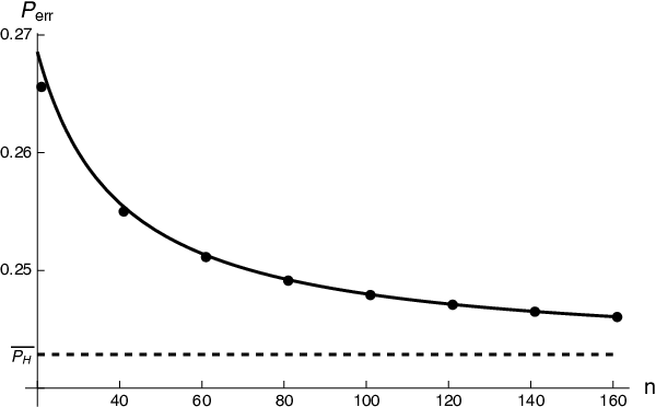
which in n→∞n\rightarrow\infty agrees with the average Helstrom probability P¯H=17/70\bar{P}_{H}=17/70 that in the present case can be obtained by integrating (III-A) with respect to r1r_{1} and r2r_{2} with the corresponding hard sphere measures. In Figure 2 we show the comparison between the exact values of Pe​r​r,m​i​n(n)P_{err,min}^{(n)} (69) and the asymptotic expansion (72).
Refer to caption
Fig. 2: Scenario ii) Minimal probability of error as a function of nn: exact values (dots), asymptotic expansion Eq. (72) (solid line), Helstrom probability (dashed line).

III-C Scenario iii): Pure states at fixed overlap

We now consider the case where the templates states ρ1=|ψ1⟩​⟨ψ1|\rho_{1}=|\psi_{1}\rangle\langle\psi_{1}| and ρ2=|ψ2⟩​⟨ψ2|\rho_{2}=|\psi_{2}\rangle\langle\psi_{2}| are pure and characterized by a mutual overlap which is known a priori. No information about the absolute orientation of the couple is instead assumed. As anticipated in the introductory section this model appears to be well suited to characterize a scenario where for instance the machine is asked to discriminate between two possible configurations on the basis of templates generated by an external party which does not share a common reference frame with the machine itself. Without loss of generality we can model this problem by setting

|ψ1⟩=|↑⟩,|ψ2⟩=U0​|↑⟩,\displaystyle|\psi_{1}\rangle=|{\uparrow}\rangle\;,\qquad|{\psi_{2}}\rangle=U_{0}|{\uparrow}\rangle\;, (73)

with a fixed unitary U0U_{0}, and then average on the action of a unitary transformation UU on both ρ1,ρ2\rho_{1},\rho_{2}. With this choice the states (4) become

α(n)=∫d​U​(U⁡|↑⟩​⟨↑|​U†)⊗n+1\displaystyle{\alpha^{(n)}}=\int dU\left({U|{\uparrow}\rangle\langle{\uparrow}|U^{\dagger}}\right)^{\otimes n+1}\!\!
⊗(U​U0​|↑⟩​⟨↑|​U0†​U†)⊗n\displaystyle\otimes\left({UU_{0}|{\uparrow}\rangle\langle{\uparrow}|U_{0}^{\dagger}U^{\dagger}}\right)^{\otimes n} (74)
β(n)=∫d​U​(U⁡|↑⟩​⟨↑|​U†)⊗n\displaystyle{\beta^{(n)}}=\int dU\left({U|{\uparrow}\rangle\langle{\uparrow}|U^{\dagger}}\right)^{\otimes n}\!\!
⊗(U​U0​|↑⟩​⟨↑|​U0†​U†)⊗n+1\displaystyle\otimes\left({UU_{0}|{\uparrow}\rangle\langle{\uparrow}|U_{0}^{\dagger}U^{\dagger}}\right)^{\otimes n+1} (75)

where once more d​UdU is the Haar measure of S​U​(2)SU(2). As in the cases analyzed before α(n){\alpha^{(n)}} and β(n){\beta^{(n)}}, as well as their difference Θ(n)\Theta^{(n)} are invariant under U⊗2​n+1U^{\otimes 2n+1}. Furthermore, since on both the A​XAX and the BB partition α(n)\alpha^{(n)} is described by pure vectors which are completely symmetric under permutations, the only elements of the basis (15) on which it can have support are those with maximum values of s′s^{\prime} and tt, i.e. s′=(n+1)/2s^{\prime}=(n+1)/2, t=n/2t=n/2. As explicitly derived in (VI-B), these states are also eigenstates for α(n)\alpha^{(n)}, i.e.

α(n)|n+12,n2;q,m⟩=Φ(n)(q,U0)|n+12,n2;q,m⟩,{\alpha^{(n)}}|{\tfrac{n+1}{2},\tfrac{n}{2};q,m}\rangle=\Phi^{(n)}(q,U_{0})|{\tfrac{n+1}{2},\tfrac{n}{2};q,m}\rangle, (76)

with eigenvalues Φ(n)​(q,U0)\Phi^{(n)}(q,U_{0}) given by

Φ(n)(q,U0)=∑h=−n/2n/2Dh,n2n2(U0)Dn2,hn2(U0†)\displaystyle\Phi^{(n)}(q,U_{0})=\sum_{h=-{n}/2}^{{n}/2}D^{\frac{n}{2}}_{h,\frac{n}{2}}(U_{0}){D^{\frac{n}{2}}_{\frac{n}{2},h}}(U_{0}^{\dagger})
×12​q+1​Cn+12,n+12,n2,hq,n+12+h​Cn+12,n+12,n2,hq,n+12+h,\displaystyle\times\frac{1}{2q+1}\;C^{q,\frac{n+1}{2}+h}_{\frac{n+1}{2},\frac{n+1}{2},\frac{n}{2},h}C^{q,\frac{n+1}{2}+h}_{\frac{n+1}{2},\frac{n+1}{2},\frac{n}{2},h},
(77)

where the symbol Dm​m′j​(U)D^{j}_{mm^{\prime}}(U) represent the matrix elements of the irreducible representations of U∈S​U​(2)U\in SU(2) with dimension 2​j+12j+1, and Cj,m,j′,m′q,lC^{q,l}_{j,m,j^{\prime},m^{\prime}} being the Clebsch-Gordan coefficients. (Notice that in the above analysis we dropped the multiplicity labels ii and kk in writing the elements of the basis (15) because for the s′=(n+1)/2s^{\prime}=(n+1)/2, t=n/2t=n/2 no degeneracy of the representation is present, #⁡(n/2,n)=1\#(n/2,n)=1). Analogous properties applies for β(n){\beta^{(n)}} when expressed into the basis (37). Therefore as in the previous cases Θ\Theta can be expressed as a direct sum of 1×11\times 1 and 2×22\times 2 block matrices. In the present case, however due to the special restriction on ss and tt instead of the four possible cases observed in the previous section, only a) and d) may occur. It turns out that for the case a) the associated eigenvalues is always null. For d) instead we have

λs=n/2,t=n/2,q(n)​(±)=±Φ(n)​(q,U0)\displaystyle\lambda^{(n)}_{s=n/2,t=n/2,q}(\pm)=\pm\Phi^{(n)}(q,U_{0})\qquad\qquad (78)
×|C+⁣−(s=n/2,t=n/2,q)|,\displaystyle\times|C^{(s=n/2,t=n/2,q)}_{+-}|,

and the eigenvectors are the same that we obtain for r1=r2=1r_{1}=r_{2}=1 in the case of completely random orientations: for pure states, the optimal POVM in the fixed overlap case is the same. Therefore, writing the eigenvalues in a simpler notation as λq(n)​(±)\lambda_{q}^{(n)}(\pm), we have

Θ(n)=∑q(λq(n)​(+)​Πq,++λq(n)​(−)​Πq,−),\Theta^{(n)}=\sum_{q}\left(\lambda^{(n)}_{q}(+)\Pi_{q,+}+\lambda^{(n)}_{q}(-)\Pi_{q,-}\right), (79)

where Πq+\Pi_{q+} and Πq−\Pi_{q-} are the projectors on eigenvectors with total angular momentum qq and respectively positive and negative eigenvalues.

Replacing all this into Eq. (10) we can finally write

Pe​r​r,m​i​n(n)=12−12​∑q(2​q+1)​λq(n)​(+),P_{err,min}^{(n)}=\frac{1}{2}-\frac{1}{2}{\sum_{q}}(2q+1)\;\lambda^{(n)}_{q}(+)\;, (80)

where we used the fact that Ms=n/2,t=n/2,q(n)=2​q+1M_{s=n/2,t=n/2,q}^{(n)}=2q+1 and that only the ++ elements of the couples (78) are positive. To proceed further, without loss of generality, we write U0=exp(−iσy(π−θ)/2)U_{0}=\exp(-i\sigma_{y}(\pi-\theta)/2) obtaining

Dh,n2n2​(U0)​Dn2,hn2​(U0†)=n!(n2+h)!​(n2−h)!\displaystyle D^{\frac{n}{2}}_{h,\frac{n}{2}}(U_{0})D^{\frac{n}{2}}_{\frac{n}{2},h}(U_{0}^{\dagger})=\frac{n!}{\left(\frac{n}{2}+h\right)!\left(\frac{n}{2}-h\right)!} (81)
×(cos2⁡(π−θ2))n2+h​(sin2⁡(π−θ2))n2−h,\displaystyle\qquad\times\left(\cos^{2}\left(\frac{\pi-\theta}{2}\right)\right)^{\frac{n}{2}+h}\left(\sin^{2}\left(\frac{\pi-\theta}{2}\right)\right)^{\frac{n}{2}-h},

which is a binomial distribution in the variable n2+h∈{0,n}\frac{n}{2}+h\in\{0,n\}. We also notice that

(Cn+12,n+12,n2,hq,n+12+h)2=2​(n2−h)!​(n+1)!(n2+h)!\displaystyle\left(C^{q,\frac{n+1}{2}+h}_{\frac{n+1}{2},\frac{n+1}{2},\frac{n}{2},h}\right)^{2}=\frac{2\left(\frac{n}{2}-h\right)!\left(n+1\right)!}{\left(\frac{n}{2}+h\right)!}
×(n2+h+q+12)!(q−12−n2−h)!​(n−q+12)!​(n+q+32)!,\displaystyle\times\frac{\left(\frac{n}{2}+h+q+\frac{1}{2}\right)!}{\left(q-\frac{1}{2}-\frac{n}{2}-h\right)!\left(n-q+\frac{1}{2}\right)!\left(n+q+\frac{3}{2}\right)!}, (82)

is also a probability distribution in the variable q∈{n2+h,n+12}q\in\{\frac{n}{2}+h,n+\frac{1}{2}\}. Then the terms entering in the sum of Eq. (80) rewrite explicitly as

(2​q+1)​λq(n)​(+)=∑hn!(n2+h)!​(n2−h)!\displaystyle(2q+1)\lambda^{(n)}_{q}(+)=\sum_{h}\frac{n!}{\left(\frac{n}{2}+h\right)!\left(\frac{n}{2}-h\right)!}
×(cos2⁡(π−θ2))n2+h​(sin2⁡(π−θ2))n2−h\displaystyle\times\left(\cos^{2}\left(\frac{\pi-\theta}{2}\right)\right)^{\frac{n}{2}+h}\left(\sin^{2}\left(\frac{\pi-\theta}{2}\right)\right)^{\frac{n}{2}-h}
×2​(n2−h)!​(n2+h+q+12)!​(n+1)!(n2−h+q−12)!​(n2+h)!​(n−q+12)!​(n+q+32)!\displaystyle\times\frac{2\left(\frac{n}{2}-h\right)!\left(\frac{n}{2}+h+q+\frac{1}{2}\right)!\left(n+1\right)!}{\left(\frac{n}{2}-h+q-\frac{1}{2}\right)!\left(\frac{n}{2}+h\right)!\left(n-q+\frac{1}{2}\right)!\left(n+q+\frac{3}{2}\right)!}
×12​2​(3/2+q+n)​(1/2−q+n)(n/2+1/2)​(n+1).\displaystyle\times\frac{1}{2}\sqrt{\frac{2(3/2+q+n)(1/2-q+n)}{(n/2+1/2)(n+1)}}\;. (83)

As usual we focus on the limit of large n≫1n\gg 1 for Pe​r​r,m​i​n(n)P_{err,min}^{(n)}. In this case we notice that in order to get up to the order O⁡(1n2)O(\frac{1}{n^{2}}) for the resulting expression, one can expand |C+⁣−(s=n/2,t=n/2,q)||C^{(s=n/2,t=n/2,q)}_{+-}| around the mean of the qq distribution and consider contributions up to the fourth central moment (see Appendix VI-C and supplementary Mathematica notebooks), expand the result around the mean of the hh distribution and calculate the contributions up to the relevant moment (not more than the fourth). The result is

Pe​r​r,m​i​n(n≫1)≃12​(1−|cos⁡θ2|)+3+cos⁡θ8​2​1+cos⁡θ​1n\displaystyle P_{err,min}^{(n\gg 1)}\simeq\frac{1}{2}\left(1-|\cos\tfrac{\theta}{2}|\right)+\tfrac{3+\cos\theta}{8\sqrt{2}\sqrt{1+\cos\theta}}\frac{1}{n}
+1−60​cos⁡θ−5​cos⁡2​θ128​2​(1+cos⁡θ)3/2​1n2,\displaystyle+\tfrac{1-60\cos\theta-5\cos 2\theta}{128\sqrt{2}(1+\cos\theta)^{3/2}}\frac{1}{n^{2}}\;, (84)

where, as expected, the first contribution corresponds to the corresponding averaged Helstrom probability P¯H\bar{P}_{H} – see also Figure  3. We notice that for small deviations from orthogonality, one has

Pe​r​r,m​i​n(n≫1)≃θ216+14​n−18​n2​(1−θ24),P_{err,min}^{(n\gg 1)}\simeq\frac{\theta^{2}}{16}+\frac{1}{4n}-\frac{1}{8n^{2}}\left(1-\frac{\theta^{2}}{4}\right)\;, (85)

The expansion around coincident states is instead singular, but the formula is still valid when the states are not coincident and n⁡(π−θ)≫1n(\pi-\theta)\gg 1. Since the optimal POVM is the same of the totally random pure state scenario, averaging over θ\theta before doing the asymptotic expansion gives the result of (60) when r1=r2=1r_{1}=r_{2}=1. Integrating at the end gives also the same result up to first order, while the order n−2{n^{-2}} is not integrable. This is not inconsistent: one can see that the averaged Pe​r​r,m​i​n(n)P^{(n)}_{err,min} displays a n−32{n^{-\frac{3}{2}}} dependence which is not recoverable from this expansion (and also not exactly computable with the Euler-MacLaurin approximation), which at fixed nn works only in the region n⁡(π−θ)≫1n(\pi-\theta)\gg 1.

Refer to caption
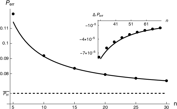
Fig. 3: Scenario iii) Minimal probability of error as a function of nn,with θ=π3\theta=\frac{\pi}{3}: exact values (dots), asymptotic expansion Eq. (84) (solid line), Helstrom probability (dashed line). In the inset we show the second order correction.

III-C1 Generalisation in finite dimension dd

For the special setting of the present scenario we present also a generalization to higher dimension. For this purpose we now consider |ψ1⟩|{\psi_{1}}\rangle and |ψ2⟩|{\psi_{2}}\rangle as states in a dd dimensional Hilbert space. Accordingly, substituting |↑⟩|{\uparrow}\rangle with |e⟩|{e}\rangle, we can write the analogue of (74), (75) as

αd(n)=∫S​U​(d)d​U​(U⁡|e⟩​⟨e|​U†)⊗n+1\displaystyle{\alpha^{(n)}_{d}}=\int_{SU(d)}dU\left({U|{e}\rangle\langle{e}|U^{\dagger}}\right)^{\otimes n+1}\!\!
⊗(U​U0​|e⟩​⟨e|​U0†​U†)⊗n\displaystyle\otimes\left({UU_{0}|{e}\rangle\langle{e}|U_{0}^{\dagger}U^{\dagger}}\right)^{\otimes n} (86)
βd(n)=∫S​U​(d)d​U​(U⁡|e⟩​⟨e|​U†)⊗n\displaystyle{\beta^{(n)}_{d}}=\int_{SU(d)}dU\left({U|{e}\rangle\langle{e}|U^{\dagger}}\right)^{\otimes n}\!\!
⊗(U​U0​|e⟩​⟨e|​U0†​U†)⊗n+1.\displaystyle\otimes\left({UU_{0}|{e}\rangle\langle{e}|U_{0}^{\dagger}U^{\dagger}}\right)^{\otimes n+1}. (87)

By the invariance of the Haar measure, one can insert for free an integration over an S​U​(2)SU(2) subgroup of S​U​(d)SU(d) which act non-trivially only on the space ℰ\mathcal{E} generated by |e⟩|{e}\rangle and U0​|e⟩U_{0}|{e}\rangle, and write

αd(n)=∫S​U​(d)d​U​∫S​U​(2)d​V​(U​V​|e⟩​⟨e|​V†​U†)⊗n+1⊗(U​V​U0​|e⟩​⟨e|​U0†​V†​U†)⊗n==∫S​U​(d)d​U​U⊗2​n+1​α2(n)​U†⊗2​n+1,{\alpha^{(n)}_{d}}=\int_{SU(d)}dU\int_{SU(2)}dV\left({UV|{e}\rangle\langle{e}|V^{\dagger}U^{\dagger}}\right)^{\otimes n+1}\!\!\\ \otimes\left({UVU_{0}|{e}\rangle\langle{e}|U_{0}^{\dagger}V^{\dagger}U^{\dagger}}\right)^{\otimes n}=\\ =\int_{SU(d)}dUU^{\otimes 2n+1}\alpha^{(n)}_{2}{U^{\dagger}}^{\otimes 2n+1}, (88)
βd(n)=∫S​U​(d)d​U​∫S​U​(2CLOSEd​V​(U​V​|e⟩​⟨e|​V†​U†)⊗n⊗(U​V​U0​|e⟩​⟨e|​U0†​V†​U†)⊗n+1==∫S​U​(d)d​U​U⊗2​n+1​β2(n)​U†⊗2​n+1,{\beta^{(n)}_{d}}=\int_{SU(d)}dU\int_{SU(2}dV\left({UV|{e}\rangle\langle{e}|V^{\dagger}U^{\dagger}}\right)^{\otimes n}\!\!\\ \otimes\left({UVU_{0}|{e}\rangle\langle{e}|U_{0}^{\dagger}V^{\dagger}U^{\dagger}}\right)^{\otimes n+1}=\\ =\int_{SU(d)}dUU^{\otimes 2n+1}\beta^{(n)}_{2}{U^{\dagger}}^{\otimes 2n+1}, (89)

with α2(n)\alpha^{(n)}_{2} and β2(n)\beta^{(n)}_{2} defined as in (74), (75), but supported on ℰ⊗2​n+1\mathcal{E}^{\otimes 2n+1}. By the same token, one has

Θd=αd(n)−βd(n)=∫S​U​(d)d​U​U⊗2​n+1​(α2(n)−β2(n))​U†⊗2​n+1=∫S​U​(d)d​U​U⊗2​n+1​Θ2​U†⊗2​n+1.\Theta_{d}=\alpha^{(n)}_{d}-\beta^{(n)}_{d}=\\ \int_{SU(d)}dUU^{\otimes 2n+1}(\alpha^{(n)}_{2}-\beta^{(n)}_{2}){U^{\dagger}}^{\otimes 2n+1}=\\ \int_{SU(d)}dUU^{\otimes 2n+1}\Theta_{2}{U^{\dagger}}^{\otimes 2n+1}. (90)

Since Schur-Weyl duality holds also for S​U​(d)SU(d), the Hilbert space of 2​n+12n+1 multiple systems still admits a decomposition

ℋ=⨁D(γD⊗μD)\mathcal{H}=\bigoplus_{D}(\gamma_{D}\otimes\mu_{D}) (91)

where γD\gamma_{D} and μD\mu_{D} are the irreducible representations of S​U​(d)SU(d) and the symmetric group S2​n+1S_{2n+1} with Young diagram DD.

Nonetheless, ℰ⊗2​n+1\mathcal{E}^{\otimes 2n+1} can be decomposed as ℰ⊗2​n+1=⨁DjD⊗μD\mathcal{E}^{\otimes 2n+1}=\bigoplus_{D}j_{D}\otimes\mu_{D} with jDj_{D}, μD\mu_{D} irreducible representations of S​U​(2)SU(2) and S2​n+1S_{2n+1} with Young diagram DD. In particular it follows that jD⊆γDj_{D}\subseteq\gamma_{D}. From (79) we know that Θ2\Theta_{2} has the form

Θ2=∑q(λq​(+)​Πq,+(ℰ)+λq​(−)​Πq,−(ℰ)),\Theta_{2}=\sum_{q}\left(\lambda_{q}(+)\Pi_{q,+}^{(\mathcal{E})}+\lambda_{q}(-)\Pi_{q,-}^{(\mathcal{E})}\right), (92)

with Πq,±(ℰ)\Pi_{q,\pm}^{(\mathcal{E})} projecting on vectors of the form |q,m⟩⊗|±⟩|{q,m}\rangle\otimes|{\pm}\rangle, with |q,m⟩∈jq,|±⟩∈μq|{q,m}\rangle\in j_{q},|{\pm}\rangle\in\mu_{q}, with qq being the associated Young diagram.

Therefore, calling Πq,+\Pi_{q,+} the projector on γq⊗|+⟩⟨+|\gamma_{q}\otimes|{+}\rangle\langle{+}| and Πq,−\Pi_{q,-} the projector on γq⊗|−⟩⟨−|\gamma_{q}\otimes|{-}\rangle\langle{-}|, we have

Θd=∫S​U​(d)d​U​U⊗2​n+1​Θ2​U†⊗2​n+1=∑qλq​(+)​∫S​U​(d)d​U​U⊗2​n+1​Πq,+(ℰ)​U⊗2​n+1+∑qλq(−)∫S​U​(d)dUU⊗2​n+1Π(ℰ)q,−U⊗2​n+1=∑q2​q+1gq(d)​(λq​(+)​Πq,++λq​(−)​Πq,−),\Theta_{d}=\int_{SU(d)}dUU^{\otimes 2n+1}\Theta_{2}{U^{\dagger}}^{\otimes 2n+1}\\ =\sum_{q}\lambda_{q}(+)\int_{SU(d)}dU{U}^{\otimes{2n+1}}\Pi^{(\mathcal{E})}_{q,+}U^{\otimes{2n+1}}\\ +\sum_{q}\lambda_{q}(-)\int_{SU(d)}dU{U}^{\otimes{2n+1}}\Pi^{(\mathcal{E})}_{q,-}U^{\otimes{2n+1}}\\ =\sum_{q}\frac{2q+1}{g_{q}^{(d)}}\left(\lambda_{q}(+)\Pi_{q,+}+\lambda_{q}(-)\Pi_{q,-}\right)\,, (93)

where we used the Peter-Weyl theorem [22] in the last equality, where now gq(d)g_{q}^{(d)} is the dimension of the representation γq\gamma_{q}. Finally, since Tr⁡[Πq,±]=gq(d)\Tr[\Pi_{q,\pm}]=g_{q}^{(d)}, the probability of error in the dd dimensional case is still (84):

Pe​r​r,m​i​n,d(n≫1)≃12​(1−|cos⁡θ2|)+3+cos⁡θ8​2​1+cos⁡θ​1n\displaystyle P_{err,min,d}^{(n\gg 1)}\simeq\frac{1}{2}\left(1-|\cos\tfrac{\theta}{2}|\right)+\tfrac{3+\cos\theta}{8\sqrt{2}\sqrt{1+\cos\theta}}\frac{1}{n}
+1−60​cos⁡θ−5​cos⁡2​θ128​2​(1+cos⁡θ)3/2​1n2,\displaystyle+\tfrac{1-60\cos\theta-5\cos 2\theta}{128\sqrt{2}(1+\cos\theta)^{3/2}}\frac{1}{n^{2}}\;, (94)

with sin⁡θ2=|⟨e|U0|e⟩|\sin\frac{\theta}{2}=|\langle{e}|U_{0}|{e}\rangle|. Also in this case one can get the probability of error of the optimal learning machines for Haar random pure states by integrating over the probability distribution of the overlap c=sin2⁡θ2c=\sin^{2}\frac{\theta}{2}, which for Haar random |ψ⟩1|{\psi}\rangle_{1} and |ψ2⟩|{\psi_{2}}\rangle is known (e.g. [31]) and equal to P⁡(c)=(d−1)​(1−c)d−2P(c)=(d-1)(1-c)^{d-2}. At the next to leading order the result is

Pe​r​r,m​i​n,d(n≫1)≃12−d−12​d−1+(d−1)23+4​d​(d−2)​1n.\displaystyle P_{err,min,d}^{(n\gg 1)}\simeq\frac{1}{2}-\frac{d-1}{2d-1}+\frac{(d-1)^{2}}{3+4d(d-2)}\frac{1}{n}\;. . (95)

which agrees with the zeroth order result in [10]. The asymptotic correction that we find can be also directly calculated by following the approach in [10], the interested reader can find the calculations in the supplementary Mathematica notebooks.

III-D Compatibility between optimal machines

In the previous subsections we have analysed three different scenarios, which in principles give rise to different optimal machines. However, additional symmetries make some of the optimal machines compatible, in the sense that it exists a measurement that is optimal for different scenarios. In particular, if S^A​B\hat{S}_{AB} is the swap operator between ℋA\mathcal{H}_{A} and ℋB\mathcal{H}_{B}, one can verify that S^A​B​α(n)​S^A​B†=β(n)\hat{S}_{AB}\alpha^{(n)}\hat{S}_{AB}^{\dagger}=\beta^{(n)} in scenario (ii), (iii) and also (i) when r1=r2r_{1}=r_{2}. If this happens then S^A​B​Θ​S^A​B†=−Θ\hat{S}_{AB}\Theta\hat{S}_{AB}^{\dagger}=-\Theta; it follows that if |λ⟩|{\lambda}\rangle is an eigenvector of Θ\Theta with eigenvalue λ\lambda, then also S^A​B​|λ⟩\hat{S}_{AB}|{\lambda}\rangle is an eigenvector, with eigenvalue −λ-\lambda. Since S^A​B|s+1/2,s;q,m⟩i,k=|s,s+1/2;q,m⟩i,k\hat{S}_{AB}|{s+1/2,s;q,m}\rangle_{i,k}=|{s,s+1/2;q,m}\rangle_{i,k}, S^A​B|s−1/2,s;q,m⟩i,k=|s,s−1/2;q,m⟩i,k\hat{S}_{AB}|{s-1/2,s;q,m}\rangle_{i,k}=|{s,s-1/2;q,m}\rangle_{i,k}, in the spaces ℋAi​X​Bk(s,s){\cal H}_{A_{i}XB_{k}}^{(s,s)} the eigenvectors are automatically determined as the orthogonal vectors |λ+⟩|{\lambda_{+}}\rangle,|λ−⟩|{\lambda_{-}}\rangle in ℋAi​X​Bk(s,s){\cal H}_{A_{i}XB_{k}}^{(s,s)} such as S^A​B​|λ+⟩=|λ−⟩\hat{S}_{AB}|{\lambda_{+}}\rangle=|{\lambda_{-}}\rangle.

In particular, since the the relevant subspace in scenario (iii) is only ℋAi​X​Bk(n2,n2){\cal H}_{A_{i}XB_{k}}^{(\frac{n}{2},\frac{n}{2})}, the optimal machine for scenario (i) when r1=r2r_{1}=r_{2}, or the one for scenario (ii), are also optimal for scenario (iii).

IV Implementation of the optimal POVM

From the knowledge of the eigenvectors (III) one can reconstruct the optimal POVM. Since it is a projective measurement, it can be realized by a change of basis from the the eigenvectors to the computational basis, followed by a local measurement. In the following we consider the implementation of the optimal machine of scenario iii), for the case n=1n=1. The change of basis is:

|ψ12,12,;32,32⟩→|↑↑↑⟩(C)\displaystyle|\psi_{\tfrac{1}{2},\tfrac{1}{2},;\tfrac{3}{2},\tfrac{3}{2}}\rangle\rightarrow|{\uparrow\uparrow\uparrow}\rangle\,\,\,\,(C)
|ψ12,12,;32,12⟩→|↑↑↓⟩(C)\displaystyle|\psi_{\tfrac{1}{2},\tfrac{1}{2},;\tfrac{3}{2},\tfrac{1}{2}}\rangle\rightarrow|{\uparrow\uparrow\downarrow}\rangle\,\,\,\,(C)
|ψ12,12,;12,12(−)⟩→|↓↑↑⟩(B)\displaystyle|\psi_{\tfrac{1}{2},\tfrac{1}{2},;\tfrac{1}{2},\tfrac{1}{2}}^{(-)}\rangle\rightarrow|{\downarrow\uparrow\uparrow}\rangle\,\,\,\,(B)
|ψ12,12,;12,12(+)⟩→|↑↓↑⟩(A)\displaystyle|\psi_{\tfrac{1}{2},\tfrac{1}{2},;\tfrac{1}{2},\tfrac{1}{2}}^{(+)}\rangle\rightarrow|{\uparrow\downarrow\uparrow}\rangle\,\,\,\,(A)
|ψ12,12,;12,−12(+)⟩→|↓↑↓⟩(A)\displaystyle|\psi_{\tfrac{1}{2},\tfrac{1}{2},;\tfrac{1}{2},-\tfrac{1}{2}}^{(+)}\rangle\rightarrow|{\downarrow\uparrow\downarrow}\rangle\,\,\,\,(A)
|ψ12,12,;12,−12(−)⟩→|↑↓↓⟩(B)\displaystyle|\psi_{\tfrac{1}{2},\tfrac{1}{2},;\tfrac{1}{2},-\tfrac{1}{2}}^{(-)}\rangle\rightarrow|{\uparrow\downarrow\downarrow}\rangle\,\,\,\,(B)
|ψ12,12,;32,−12⟩→|↓↓↑⟩(C)\displaystyle|\psi_{\tfrac{1}{2},\tfrac{1}{2},;\tfrac{3}{2},-\tfrac{1}{2}}\rangle\rightarrow|{\downarrow\downarrow\uparrow}\rangle\,\,\,\,(C)
|ψ12,12,;32,−32⟩→|↓↓↓⟩(C)\displaystyle|\psi_{\tfrac{1}{2},\tfrac{1}{2},;\tfrac{3}{2},-\tfrac{3}{2}}\rangle\rightarrow|{\downarrow\downarrow\downarrow}\rangle\,\,\,\,(C)

where AA (BB) means that the result of the measurement is interpreted as X=AX=A (X=BX=B), while for CC we ”flip a coin” to decide. In the computational basis the unitary rotation reads

(1000000001313013000013−3−3603−36000000−3−36013+31300133−360−3−360000003−3601−3+31300001301313000000001),\displaystyle\left(\begin{smallmatrix}1&0&0&0&0&0&0&0\\ 0&\frac{1}{\sqrt{3}}&\frac{1}{\sqrt{3}}&0&\frac{1}{\sqrt{3}}&0&0&0\\ 0&\frac{1}{\sqrt{3}}&\frac{-3-\sqrt{3}}{6}&0&\frac{3-\sqrt{3}}{6}&0&0&0\\ 0&0&0&\frac{-3-\sqrt{3}}{6}&0&\frac{1}{3+\sqrt{3}}&\frac{1}{\sqrt{3}}&0\\ 0&\frac{1}{\sqrt{3}}&\frac{3-\sqrt{3}}{6}&0&\frac{-3-\sqrt{3}}{6}&0&0&0\\ 0&0&0&\frac{3-\sqrt{3}}{6}&0&\frac{1}{-3+\sqrt{3}}&\frac{1}{\sqrt{3}}&0\\ 0&0&0&\frac{1}{\sqrt{3}}&0&\frac{1}{\sqrt{3}}&\frac{1}{\sqrt{3}}&0\\ 0&0&0&0&0&0&0&1\end{smallmatrix}\right), (97)

and the probability of error as a function of θ\theta is

Pe​r​r,m​i​n(1)=12−1+cos⁡θ4​3.P_{err,min}^{(1)}=\frac{1}{2}-\frac{1+\cos\theta}{4\sqrt{3}}. (98)

These kind of operations are suitable for all programmable devices which are based on the circuit model of quantum computation, as for example the recent quantum chips developed by IBM [34]. By using the software development kit QISKit [35], we have determined a circuit that realises the POVM for the n=1n=1 case with input pure states and checked its performance with the IBM simulator. The number of gates of our implementation is 6161 single qubit operations and 6060 CNOT, with a depth of 4343 operations. Given that the failure probability of a CNOT on real machines is about 5∗10−25*10^{-2}, the failure probability of the circuit is at least 1−0.9560≈0.9541-0.95^{60}\approx 0.954. Indeed we tried to remotely perform the experiment on the real physical chip, without any significant results. This fact underlines the importance of gate optimisation and error correction for the proper operation of future quantum computers. However, with the simulation tools of QISKit Aer, we were able to simulate the circuit with an error model consisting in depolarising errors (Fig. 4) and thermal relaxation errors (Fig. 5): decreasing the depolarising probability and increasing the relaxation times we can show how the circuit is sensitive to this kind of noises, and that we recover the expected behaviour for small noise.

Refer to caption
Fig. 4: Simulation of the optimal machine with QISKit Aer, with depolarising error modeled after the gate average infidelity of each gate: pfp_{f} are the depolarising probability for the 16 qubit machine (Melbourne) if all the infidelity is due to a depolarising channel. Frequency of misclassification errors with 256 repetitions for each θ\theta, compared with the predicted minimum error function (solid line).
Refer to caption
Fig. 5: Simulation of the optimal machine with QISKit Aer, with thermal relaxation times T1=T2=TT_{1}=T_{2}=T equal for each qubit. Gate times are set to 200​n​s200\,ns for 1 qubit gates and 800​n​s800\,ns for CNOT. Frequency of misclassification errors with 256 repetitions for each θ\theta, compared with the predicted minimum error function (solid line).

V Conclusions

In this work we have discussed the performances of optimal universal learning quantum machines that aim at discriminating the states of a qudit starting from a collection of templates states in the hybrid, yet realistic scenario, where at least some global information on the training set is classically available. As a matter of fact, it is not hard to identify situations for which this kind of approach could provide a realistic modelisation. Indeed, while absolute information about quantum states is typically not accessible, some structural properties are more likely to be available. For instance this is what happens in quantum communication [32] where the receiving party does not know the particular state is going to receive, but has classical knowledge on the code the sender is using. Like classical supervised learning is a fundamental tool with classical data, arguably quantum learning machines will be important for dealing with quantum data with quantum processors. Indeed, given that quantum tomography is very expensive in terms of resources, dealing with quantum data requires to study alternatives which need little information about the data, make use of the full power of quantum mechanics, and extract only the relevant information for the problem at hand. Our work extends the previous results considering more general scenarios. An interesting observation is that the optimal machine that does not assume any kind of information about the template state, scenario (ii), it is also optimal for scenario (iii), where the template states are assumed to be pure. It is therefore a very general machine, which can be seen as the most convenient learning algorithm.

Acknowledgements

The Authors thank Gael Sentís for a careful reading of the manuscript and fruitful comments.

References

  • [1] S. Shalev-Shwartz and S. Ben-David, Understanding Machine Learning: From Theory to Algorithms. (Cambridge University Press, New York, NY, USA, 2014).
  • [2] P. Wittek, Quantum machine learning: what quantum computing means to data mining (Academic Press, 2014).
  • [3] M. Schuld, I. Sinayskiy, and F. Petruccione, Contemporary Physics 56.2, 172-185 (2015).
  • [4] V. Dunjko and H. J. Briegel, Eprint arXiv:1709.02779.
  • [5] J. Biamonte, P. Wittek, N. Pancotti, P. Rebentrost, N. Wiebe and S. Lloyd, Nature 549, 195-202 (2017).
  • [6] C. Ciliberto, M. Herbster, A. D. Ialongo, M. Pontil, A. Rocchetto, S. Severini, L. Wossnig Proc. R. Soc. A 474 20170551 (2018).
  • [7] A. Monràs, G. Sentís, and P. Wittek, Phys. Rev. Lett., 118 190503 (2017).
  • [8] M. Sasaki, A. Carlini, and R. Jozsa, Phys. Rev. A, 64 022317 (2001).
  • [9] M. Sasaki and A. Carlini, Phys. Rev. A, 66 022303 (2002).
  • [10] A. Hayashi, M. Horibe, and T. Hashimoto, Phys. Rev. A, 72 052306 (2005).
  • [11] A. Hayashi, M. Horibe, and T. Hashimoto, Phys. Rev. A, 73 012328 (2006).
  • [12] S. Gambs, Eprint arXiv:0809.0444.
  • [13] C.W. Helstrom, Quantum Detection and Estimation Theory (Academic, New York, 1976).
  • [14] A. S. Holevo, J. Multivariate Anal. 3, 337 (1973).
  • [15] H. P. Yuen, R. S. Kennedy and M. Lax, IEEE Trans. Info. Theory 21, 125 (1975).
  • [16] W. K. Wootters and W. H. Zurek, Nature 299, 802 (1982).
  • [17] J. A. Bergou and M. Hillery, Phys. Rev. Lett., 94, 160501 (2005).
  • [18] M. Guţǎ and W. Kotłowski, New Journal of Physics, 12 (12) 123032 (2010).
  • [19] G. Sentís, E. Bagan, J. Calsamiglia, and R. Muñoz-Tapia, Phys. Rev. A 82 042312 (2010).
  • [20] D. A. Varshalovich, A. N. Moskalev, and V. K. Khersonskii, Quantum Theory of Angular Momentum, World Scientific, Singapore, (1988).
  • [21] W. Fulton and J. Harris, Representation theory. A first course. Graduate Texts in Mathematics, Readings in Mathematics. 129. New York: Springer-Verlag (1991).
  • [22] A. W. Knapp, Lie Groups Beyond an Introduction Birkhauser-Verlag, Basel, (1996).
  • [23] G. Sentís, J. Calsamiglia, R. Muñoz-Tapia, Scientific Reports, 2 708 (2012).
  • [24] G. Sentís, E. Bagan, J. Calsamiglia and R. Muñoz-Tapia, Phys. Rev. A, 88 052304 (2013).
  • [25] G. Sentís, M. Guţǎ, and G. Adesso, EPJ Quantum Technology, 2 (17) (2015).
  • [26] A. Peres and W. K. Wootters, Phys. Rev. Lett., 66, 1119 (1991).
  • [27] S. Massar and S. Popescu, Phys. Rev. Lett., 74, 1259 (1995).
  • [28] N. Gisin and S. Popescu, Phys. Rev. Lett., 83, 432 (1999).
  • [29] S. Massar, Phys. Rev. A, 62, 040101 (2000).
  • [30] G. Chiribella, G. M. D’Ariano, P. Perinotti, and M. F. Sacchi, Phys. Rev. Lett. 93, 180503 (2004).
  • [31] L. Alonso and T. Gorin, Journal of Physics A: Mathematical and Theoretical 49, 145004 (2016).
  • [32] A. S. Holevo, Quantum Systems, Channels, Information (de Gruyter Studies in Mathematical Physics, 2012).
  • [33] Wolfram Research, Inc., Mathematica, Version 11.3, Champaign, IL (2018).
  • [34] IBM, Quantum Experience, URL: https://www.research.ibm.com/ibm-q.
  • [35] IBM, Quantum Information Software Kit (QISKit), URL:https://www.qiskit.org.
  • [36] https://github.com/fanizzamarco/quantum-learning-machines

VI Appendix

In this appendix we present the explicit derivation of some important identities which are used in the main text. We recall that the Haar measure d​UdU of S​U​(2)SU(2) satisfies the identity

∫d​U​ℱ​(L​U)=∫d​U​ℱ​(U)=∫d​U​ℱ​(U​R),\int dU\,{\cal F}(LU)=\int dU\,{\cal F}(U)=\int dU\,{\cal F}(UR)\;,

for all L,R∈S​U​(2)L,R\in SU(2) and for all functions ℱ\cal F acting on S​U​(2)SU(2), and that it induces a Hilbert product on L2​[U,d​U]L_{2}[U,dU] via the identification

(f,g)≡∫d​U​f∗​(U)​g​(U).({f},{g})\equiv\int dU\,f^{*}(U)g(U)\;.

Furthemore, indicating with Dm,m′j​(U)D^{j}_{m,m^{\prime}}(U) the matrix elements of the irreducible representations of U∈S​U​(2)U\in SU(2) with Casimir j⁡(j+1)j(j+1), we recall that via the Peter-Weyl theorem they fulfil the identities

∫d​U​(Dm1,m1′j1​(U))∗​Dm2,m2′j2​(U)\displaystyle\int dU\,{\left(D^{j_{1}}_{m_{1},m_{1}^{\prime}}(U)\right)}^{*}D^{j_{2}}_{m_{2},m_{2}^{\prime}}(U) (99)
=12​j1+1​δj1​j2​δm1​m2​δm1′​m2′.\displaystyle\qquad\qquad\qquad=\frac{1}{2j_{1}+1}\delta_{j_{1}j_{2}}\delta_{m_{1}m_{2}}\delta_{m_{1}^{\prime}m_{2}^{\prime}}\;.

VI-A Derivation of Eq. (31)

Let ρ\rho a qubit density matrix characterized by Bloch vector of length rr which, without loss of generality we shall assume to be oriented in the positive z^\hat{z} direction, i.e. ρ=(1+r2)​|↑⟩​⟨↑|+(1−r2)|↓⟩​⟨↓|\rho=\left(\frac{1+r}{2}\right)|{\uparrow}\rangle\langle{\uparrow}|+\left(\frac{1-r}{2}\right)|{\downarrow}\rangle\langle{\downarrow}| with |↑⟩|{\uparrow}\rangle, |↓⟩|{\downarrow}\rangle being the eigenvectors of σz\sigma_{z}. We notice that its nn-th tensor power can be expressed as

ρ⊗n=∑l=0n(1+r2)l​(1−r2)n−l​Bl(n),\displaystyle\rho^{\otimes n}=\sum_{l=0}^{n}\left(\frac{1+r}{2}\right)^{l}\left(\frac{1-r}{2}\right)^{n-l}B^{(n)}_{l},

with

Bl(n)≡∑πSπ​(|↑⟩​⟨↑|⊗l⊗|↓⟩​⟨↓|⊗n−l)​Sπ†,\displaystyle B^{(n)}_{l}\equiv\sum_{\pi}S_{\pi}\left(|{\uparrow}\rangle\langle{\uparrow}|^{\otimes l}\otimes|{\downarrow}\rangle\langle{\downarrow}|^{\otimes n-l}\right)S^{\dagger}_{\pi}\;,

the sum being performed over the set of permutations operators SπS_{\pi} of nn elements. By construction Bl(n)B^{(n)}_{l} is the projector on the eigenspace at fixed total angular momentum JzJ_{z}, therefore it is diagonal in every basis of eigenvectors of J2,JzJ^{2},J_{z}. In particular its support is given by the vectors |j,l−n2⟩i|{j,l-\frac{n}{2}}\rangle_{i} in each representation with Casimir number J2=j⁡(j+1)J^{2}=j(j+1) and l∈{n2−j,⋯,n2+j}l\in\{\frac{n}{2}-j,\cdots,\frac{n}{2}+j\}, the index ii labelling accounting for the multiplicity of the representation, i.e.

Bl(n)=⊕j≥|l−n2|⊕i|j,l−n2⟩i⟨j,l−n2|.\displaystyle B^{(n)}_{l}=\oplus_{j\geq|l-\tfrac{n}{2}|}\oplus_{i}|{j,l-\tfrac{n}{2}}\rangle_{i}\langle{j,l-\tfrac{n}{2}}|\;. (100)

Consider then the operator

γ(n)\displaystyle\gamma^{(n)} ≡\displaystyle\equiv ∫d​U​(U​ρ​U†)⊗n\displaystyle\int dU\left(U\rho U^{\dagger}\right)^{\otimes n} (101)
=\displaystyle= ∑l=0n(1+r2)l​(1−r2)n−l​Pl(n),\displaystyle\sum_{l=0}^{n}\left(\frac{1+r}{2}\right)^{l}\left(\frac{1-r}{2}\right)^{n-l}P^{(n)}_{l},

with

Pl(n)\displaystyle P^{(n)}_{l} ≡\displaystyle\equiv ∫d​U​U⊗n​Bl(n)​U†⊗n.\displaystyle\int dUU^{\otimes n}B^{(n)}_{l}{U^{\dagger}}^{\otimes n}\;. (102)

Invoking the identity (99) we can conclude that

Pl(n)\displaystyle P^{(n)}_{l} =\displaystyle= ⊕j≥|l−n2|𝟏(j)2​j+1,\displaystyle\oplus_{j\geq|l-\tfrac{n}{2}|}\frac{\mathbf{1}^{(j)}}{2j+1}, (103)

where now 𝟏(j)\mathbf{1}^{(j)} is the projector on all irreducible representation with principal quantum number jj. Accordingly we have

γ(n)\displaystyle\gamma^{(n)} =\displaystyle= ⊕∑l=n2−jn2+jj⁡(1+r2)l​(1−r2)n−l​𝟏(j)2​j+1\displaystyle\oplus_{j}{\sum_{l=\tfrac{n}{2}-j}^{\tfrac{n}{2}+j}\left(\frac{1+r}{2}\right)^{l}\left(\frac{1-r}{2}\right)^{n-l}}\frac{\mathbf{1}^{(j)}}{2j+1} (104)
=\displaystyle= ⊕jfj(n)(r)𝟏(j),\displaystyle\oplus_{j}f_{j}^{(n)}(r)\mathbf{1}^{(j)},

with fj(n)​(r)f_{j}^{(n)}(r) as in (30). Equation (31) finally follows from by a direct application of (104) to the terms ∫d​U​(U​ρ1​U†)⊗n+1\int dU\left(U\rho_{1}U^{\dagger}\right)^{\otimes n+1} and ∫d​U​(U​ρ2​U†)⊗n\int dU\left(U\rho_{2}U^{\dagger}\right)^{\otimes n} that enter in the definition of the operator α(n)\alpha^{(n)} of Sec. III-A.

VI-B Derivation of Eq. (77)

To derive (77) let us first expand |n+12,n2;q,m⟩|{\tfrac{n+1}{2},\tfrac{n}{2};q,m}\rangle into the angular momentum basis given by the tensor product states |n+12,m′⟩⊗|n2,m−m′⟩|{\frac{n+1}{2},m^{\prime}}\rangle\otimes|{\frac{n}{2},m-m^{\prime}}\rangle associated with the A​X/BAX/B partition, i.e.

|n+12,n2;q,m⟩\displaystyle|{\tfrac{n+1}{2},\tfrac{n}{2};q,m}\rangle =\displaystyle= ∑m′Cn+12,m′,n2,m−m′q,m\displaystyle\sum_{m^{\prime}}C^{q,m}_{\frac{n+1}{2},m^{\prime},\frac{n}{2},m-m^{\prime}} (105)
×|n+12,m′⟩⊗|n2,m−m′⟩,\displaystyle\times|{\frac{n+1}{2},m^{\prime}}\rangle\otimes|{\frac{n}{2},m-m^{\prime}}\rangle\;,

where Cn+12,m′,n2,m−m′q,mC^{q,m}_{\frac{n+1}{2},m^{\prime},\frac{n}{2},m-m^{\prime}} are the corresponding Clebsch-Gordan coefficients. Then observing that in this basis the state |↑⟩⊗n+1⊗|↑⟩⊗n|{\uparrow}\rangle^{\otimes n+1}\otimes|{\uparrow}\rangle^{\otimes n} corresponds to the element |n+12,n+12⟩⊗|n2,n2⟩|{\tfrac{n+1}{2},\tfrac{n+1}{2}}\rangle\otimes|{\tfrac{n}{2},\tfrac{n}{2}}\rangle, we write the operator α(n)\alpha^{(n)} as

α(n)=∫dUU⊗n+1|n+12,n+12⟩⟨n+12,n+12|U†⊗n+1\displaystyle{\alpha^{(n)}}=\int dUU^{\otimes n+1}|{\tfrac{n+1}{2},\tfrac{n+1}{2}}\rangle\langle{\tfrac{n+1}{2},\tfrac{n+1}{2}}|{U^{\dagger}}^{\otimes n+1}
⊗(UU0)⊗n|n2,n2⟩⟨n2,n2|(U0†U†)⊗n,\displaystyle\otimes(UU_{0})^{\otimes n}|{\tfrac{n}{2},\tfrac{n}{2}}\rangle\langle{\tfrac{n}{2},\tfrac{n}{2}}|({U_{0}^{\dagger}U^{\dagger}})^{\otimes n}\;,

and observe that

α(n)(|n+12,m′⟩⊗|n2,m−m′⟩)=\displaystyle\!\!\!{\alpha^{(n)}}\left(|{\tfrac{n+1}{2},m^{\prime}}\rangle\otimes|{\tfrac{n}{2},m-m^{\prime}}\rangle\right)= (106)
=\displaystyle= ∑l,l′∫d​U​Dl,n+12n+12​(U)​Dn+12,m′n+12​(U†)\displaystyle\!\!\!\sum_{l,l^{\prime}}\int dUD^{\frac{n+1}{2}}_{l,\frac{n+1}{2}}(U){D^{\frac{n+1}{2}}_{\frac{n+1}{2},m^{\prime}}}(U^{\dagger})
×\displaystyle\times Dl′,n2n2(UU0)Dn2,m−m′n2(U0†U†)|n+12,l⟩⊗|n2,l′⟩\displaystyle D^{\frac{n}{2}}_{l^{\prime},\frac{n}{2}}(UU_{0}){D^{\frac{n}{2}}_{\frac{n}{2},m-m^{\prime}}}(U_{0}^{\dagger}U^{\dagger})|{\tfrac{n+1}{2},l}\rangle\otimes|{\tfrac{n}{2},l^{\prime}}\rangle
=\displaystyle= ∑h,kDh,n2n2​(U0)​Dn2,kn2​(U0†)\displaystyle\!\!\!\sum_{h,k}D^{\frac{n}{2}}_{h,\frac{n}{2}}(U_{0}){D^{\frac{n}{2}}_{\frac{n}{2},k}}(U_{0}^{\dagger})
×\displaystyle\times ∑l,l′∫d​U​Dl,n+12n+12​(U)​Dn+12,m′n+12​(U†)\displaystyle\sum_{l,l^{\prime}}\int dUD^{\frac{n+1}{2}}_{l,\frac{n+1}{2}}(U){D^{\frac{n+1}{2}}_{\frac{n+1}{2},m^{\prime}}}(U^{\dagger})
×\displaystyle\times Dl′,hn2(U)Dk,m−m′n2(U†)|n+12,l⟩⊗|n2,l′⟩,\displaystyle D^{\frac{n}{2}}_{l^{\prime},h}(U){D^{\frac{n}{2}}_{k,m-m^{\prime}}}(U^{\dagger})|{\tfrac{n+1}{2},l}\rangle\otimes|{\tfrac{n}{2},l^{\prime}}\rangle\;,

where in the first identity the matrix elements

Dm1,m2n+12​(U)=⟨n+12,m1​|U⊗n+1|​n+12,m2⟩,D^{\frac{n+1}{2}}_{m_{1},m_{2}}(U)=\langle{\frac{n+1}{2},m_{1}}|U^{\otimes{n+1}}|{\frac{n+1}{2},m_{2}}\rangle,

and

Dm1,m2n2​(U)=⟨n2,m1​|U⊗n|​n2,m2⟩,D^{\frac{n}{2}}_{m_{1},m_{2}}(U)=\langle{\frac{n}{2},m_{1}}|U^{\otimes{n}}|{\frac{n}{2},m_{2}}\rangle,

represent the action of the unitary UU into the selected basis, while in the second we used the composition rules of S​U​(2)SU(2) to factorize the contributions of U0U_{0} from the rest. This equation can be further simplified by exploiting once more the Clebsch-Gordan mapping (105) to merge together Dl,n+12n+12​(U)D^{\frac{n+1}{2}}_{l,\frac{n+1}{2}}(U) with Dl′,hn2​(U)D^{\frac{n}{2}}_{l^{\prime},h}(U), and Dn+12,m′n+12​(U†){D^{\frac{n+1}{2}}_{\frac{n+1}{2},m^{\prime}}}(U^{\dagger}) with Dk,m−m′n2​(U†){D^{\frac{n}{2}}_{k,m-m^{\prime}}}(U^{\dagger}). As a result the previous expression becomes

α(n)(|n+12,m′⟩⊗|n2,m−m′⟩)\displaystyle\!\!\!{\alpha^{(n)}}\left(|{\tfrac{n+1}{2},m^{\prime}}\rangle\otimes|{\tfrac{n}{2},m-m^{\prime}}\rangle\right)
=∑h,kDh,n2n2​(U0)​Dn2,kn2​(U0†)\displaystyle=\sum_{h,k}D^{\frac{n}{2}}_{h,\frac{n}{2}}(U_{0}){D^{\frac{n}{2}}_{\frac{n}{2},k}}(U_{0}^{\dagger})
×∑l,l′,q,q′∫d​U​Dl+l′,n+12+hq​(U)​Dn+12+k,mq′​(U†)\displaystyle\times\sum_{l,l^{\prime},q,q^{\prime}}\int dUD^{q}_{l+l^{\prime},\frac{n+1}{2}+h}(U)D^{q^{\prime}}_{\frac{n+1}{2}+k,{m}}(U^{\dagger})
×Cn+12,l,n2,l′q,l+l′​Cn+12,n+12,n2,hq,n+12+h\displaystyle\times C^{{q},l+l^{\prime}}_{\frac{n+1}{2},l,\frac{n}{2},l^{\prime}}C^{{q},\frac{n+1}{2}+h}_{\frac{n+1}{2},\frac{n+1}{2},\frac{n}{2},h}
×Cn+12,m′,n2,m−m′q′,mCn+12,n+12,n2,kq′,n+12+k|n+12,l⟩⊗|n2,l′⟩\displaystyle\times C^{{q^{\prime}},{m}}_{\frac{n+1}{2},m^{\prime},\frac{n}{2},{m}-m^{\prime}}C^{{q^{\prime}},\frac{n+1}{2}+k}_{\frac{n+1}{2},\frac{n+1}{2},\frac{n}{2},k}|{\tfrac{n+1}{2},l}\rangle\otimes|{\tfrac{n}{2},l^{\prime}}\rangle
=∑l,q12​q+1​∑hDh,n2n2​(U0)​Dn2,hn2​(U0†)\displaystyle=\sum_{l,q}\frac{1}{2q+1}\sum_{h}D^{\frac{n}{2}}_{h,\frac{n}{2}}(U_{0}){D^{\frac{n}{2}}_{\frac{n}{2},h}}(U_{0}^{\dagger})
×Cn+12,m′,n2,m−m′q,m​Cn+12,n+12,n2,hq,n+12+h\displaystyle\times C^{{q},{m}}_{\frac{n+1}{2},m^{\prime},\frac{n}{2},{m}-m^{\prime}}C^{{q},\frac{n+1}{2}+h}_{\frac{n+1}{2},\frac{n+1}{2},\frac{n}{2},h}
×Cn+12,n+12,n2,hq,n+12+hCn+12,l,n2,m−lq,m|n+12,l⟩⊗|n2,m−l⟩,\displaystyle\times C^{{q},\frac{n+1}{2}+h}_{\frac{n+1}{2},\frac{n+1}{2},\frac{n}{2},h}C^{{q},{m}}_{\frac{n+1}{2},l,\frac{n}{2},m-l}|{\tfrac{n+1}{2},l}\rangle\otimes|{\tfrac{n}{2},m-l}\rangle\;,

where in the second identity we exploit the Peter-Weyl theorem, see Eq. (99), to evaluate the integral in UU, obtaining that the nonzero terms in the sum have to satisfy q=q′q=q^{\prime}, l+l′=ml+l^{\prime}=m, h=kh=k. Multiplying this by Cn+12,m′,n2,m−m′q,mC^{q,m}_{\frac{n+1}{2},m^{\prime},\frac{n}{2},m-m^{\prime}} while summing over m′m^{\prime}, the latter equation finally gives us

α(n)|n+12,n2;q,m⟩\displaystyle\!\!\!{\alpha^{(n)}}|{\tfrac{n+1}{2},\tfrac{n}{2};q,m}\rangle
=∑l,m′,q′12​q′+1​∑hDh,n2n2​(U0)​Dn2,hn2​(U0†)\displaystyle=\sum_{l,m^{\prime},q^{\prime}}\frac{1}{2q^{\prime}+1}\sum_{h}D^{\frac{n}{2}}_{h,\frac{n}{2}}(U_{0}){D^{\frac{n}{2}}_{\frac{n}{2},h}}(U_{0}^{\dagger})
×Cn+12,m′,n2,m−m′q,m​Cn+12,m′,n2,m−m′q′,m\displaystyle\times C^{q,m}_{\frac{n+1}{2},m^{\prime},\frac{n}{2},m-m^{\prime}}C^{{q^{\prime}},{m}}_{\frac{n+1}{2},m^{\prime},\frac{n}{2},{m}-m^{\prime}}
×Cn+12,n2,n2,hq′,n+12+h​Cn+12,n+12,n2,hq′,n+12+h\displaystyle\times\,C^{{q^{\prime}},\frac{n+1}{2}+h}_{\frac{n+1}{2},\frac{n}{2},\frac{n}{2},h}C^{{q^{\prime}},\frac{n+1}{2}+h}_{\frac{n+1}{2},\frac{n+1}{2},\frac{n}{2},h}
×Cn+12,l,n2,m−lq′,m|n+12,l⟩⊗|n2,m−l⟩,\displaystyle\times\,C^{{q^{\prime}},{m}}_{\frac{n+1}{2},l,\frac{n}{2},m-l}|{\tfrac{n+1}{2},l}\rangle\otimes|{\tfrac{n}{2},m-l}\rangle\;,
=12​q+1​∑hDh,n2n2​(U0)​Dn2,hn2​(U0†)\displaystyle=\frac{1}{2{q}+1}\sum_{h}D^{\frac{n}{2}}_{h,\frac{n}{2}}(U_{0}){D^{\frac{n}{2}}_{\frac{n}{2},h}}(U_{0}^{\dagger})
×Cn+12,n+12,n2,hq,n+12+hCn+12,n+12,n2,hq,n+12+h|n+12,n2;q,m⟩,\displaystyle\times\,C^{{q},\frac{n+1}{2}+h}_{\frac{n+1}{2},\frac{n+1}{2},\frac{n}{2},h}C^{{q},\frac{n+1}{2}+h}_{\frac{n+1}{2},\frac{n+1}{2},\frac{n}{2},h}|{\tfrac{n+1}{2},\tfrac{n}{2};q,m}\rangle\;,

which coincides with (77). Here in the second equality we used the orthogonality of the Clebsch-Gordan coefficients to select only the term q′=qq^{\prime}=q in the sum.

VI-C Central momenta of the distributions

Here we report the central momenta of the distributions used for computing (84).

Putting h=n​s2h=\frac{ns}{2} and 1+r2=cos⁡(π−θ2)\frac{1+r}{2}=\cos\left(\frac{\pi-\theta}{2}\right) we notice that the distribution

Pθ(n)​(s)\displaystyle P_{\theta}^{(n)}(s) ≡\displaystyle\equiv Dh,n2n2​(U0)​Dn2,hn2​(U0†),\displaystyle D^{\frac{n}{2}}_{h,\frac{n}{2}}(U_{0})D^{\frac{n}{2}}_{\frac{n}{2},h}(U_{0}^{\dagger})\;, (108)

defined in Eq. (81) has momenta

μ1\displaystyle\mu_{1} =\displaystyle= E⁡[s]=r,\displaystyle E[s]=r\;,
μ2\displaystyle\mu_{2} =\displaystyle= E⁡[(s−μ1)2]=1−r2n,\displaystyle E[(s-\mu_{1})^{2}]=\frac{1-r^{2}}{n}\;,
μ3\displaystyle\mu_{3} =\displaystyle= E⁡[(s−μ1)3]=2​r​1−r2n,\displaystyle E[(s-\mu_{1})^{3}]=2r\frac{1-r^{2}}{n}\;,
μ4\displaystyle\mu_{4} =\displaystyle= E⁡[(s−μ1)4]\displaystyle E[(s-\mu_{1})^{4}]
=\displaystyle= (−1+r2)​(2−6​r2+3​n​(−1+r2))n3.\displaystyle\frac{(-1+r^{2})(2-6r^{2}+3n(-1+r^{2}))}{n^{3}}\;.

Instead, setting h=n​s2h=\frac{ns}{2}, we notice that the momenta of the distribution

Ph(n)​(q)≡2​(n2−h)!​(n+1)!(n2+h)!\displaystyle P^{(n)}_{h}(q)\equiv\frac{2\left(\frac{n}{2}-h\right)!\left(n+1\right)!}{\left(\frac{n}{2}+h\right)!}
×(n2+h+q+12)!(q−12−n2−h)!​(n−q+12)!​(n+q+32)!,\displaystyle\times\frac{\left(\frac{n}{2}+h+q+\frac{1}{2}\right)!}{\left(q-\frac{1}{2}-\frac{n}{2}-h\right)!\left(n-q+\frac{1}{2}\right)!\left(n+q+\frac{3}{2}\right)!}\;,

defined in (82), can be expressed in terms of Euler gamma functions as follows

μ1\displaystyle\mu_{1} =\displaystyle= E⁡[q]\displaystyle E[q]
=\displaystyle= −12+Γ⁡(1/2+h+n/2)​Γ​(2+n)Γ⁡(1+h+n/2)​Γ​(3/2+n)\displaystyle-\frac{1}{2}+\frac{\Gamma(1/2+h+n/2)\Gamma(2+n)}{\Gamma(1+h+n/2)\Gamma(3/2+n)}
=\displaystyle= n​1+s2−12\displaystyle\frac{n\sqrt{1+s}}{\sqrt{2}}-\frac{1}{2}
+\displaystyle+ 11+5​s8​2​1+s+9+14​s−23​s2128​2​n​(1+s)3/2\displaystyle\frac{11+5s}{8\sqrt{2}\sqrt{1+s}}+\frac{9+14s-23s^{2}}{128\sqrt{2}n(1+s)^{3/2}}
+\displaystyle+ O⁡(1n2),\displaystyle O\left(\frac{1}{n^{2}}\right)\;,
μ2\displaystyle\mu_{2} =\displaystyle= E⁡[(q−μ1)2]\displaystyle E[(q-\mu_{1})^{2}]
=\displaystyle= 12​(1+n)​(2+2​h+n)\displaystyle\frac{1}{2}(1+n)(2+2h+n)
−\displaystyle- Γ​(3/2+h+n/2)2​Γ​(2+n)2Γ​(1+h+n/2)2​Γ​(3/2+n)2\displaystyle\frac{\Gamma(3/2+h+n/2)^{2}\Gamma(2+n)^{2}}{\Gamma(1+h+n/2)^{2}\Gamma(3/2+n)^{2}}
=\displaystyle= 18​n​(1−s)+−1+2​s−s264​(1+s)+O⁡(1n)\displaystyle\frac{1}{8}n(1-s)+\frac{-1+2s-s^{2}}{64(1+s)}+O\left(\frac{1}{n}\right)
μ3=E⁡[(q−μ1)3]\displaystyle\mu_{3}=E[(q-\mu_{1})^{3}]
=−(8+2​h​(5+4​n)+n⁡(11+4​n))​Γ​(3/2+h+n/2)​Γ​(2+n)Γ⁡(1+h+n/2)​Γ​(3/2+n)\displaystyle=\frac{-(8+2h(5+4n)+n(11+4n))\Gamma(3/2+h+n/2)\Gamma(2+n)}{\Gamma(1+h+n/2)\Gamma(3/2+n)}
+8​Γ​(3/2+h+n/2)3​Γ​(2+n)34​Γ​(1+h+n/2)3​Γ​(3/2+n)3\displaystyle+\frac{8\Gamma(3/2+h+n/2)^{3}\Gamma(2+n)^{3}}{4\Gamma(1+h+n/2)^{3}\Gamma(3/2+n)^{3}}
=(−1+s)2​n32​2​1+s+O⁡(1),\displaystyle=\frac{(-1+s)^{2}n}{32\sqrt{2}\sqrt{1+s}}+O\left(1\right)\;,
μ4=E⁡[(q−μ1)4]\displaystyle\mu_{4}=E[(q-\mu_{1})^{4}]
=(1+n)​(4+10​n+4​h2​n+6​n2+n3+4​h​(1+3​n+n2))4\displaystyle=\frac{(1+n)(4+10n+4h^{2}n+6n^{2}+n^{3}+4h(1+3n+n^{2}))}{4}
−3​Γ​(3/2+h+n/2)4​Γ​(2+n)4Γ​(1+h+n/2)4​Γ​(3/2+n)4\displaystyle-\frac{3\Gamma(3/2+h+n/2)^{4}\Gamma(2+n)^{4}}{\Gamma(1+h+n/2)^{4}\Gamma(3/2+n)^{4}}
+(2+2​n+n2+2​h​(2+n))​π2​Γ​(2+2​h+n)2​Γ​(3+2​n)243+2​h+3​n​Γ​(1+h+n/2)4​Γ​(3/2+n)4\displaystyle+\frac{(2+2n+n^{2}+2h(2+n))\pi^{2}\Gamma(2+2h+n)^{2}\Gamma(3+2n)^{2}}{4^{3+2h+3n}\Gamma(1+h+n/2)^{4}\Gamma(3/2+n)^{4}}
=36​4​(1−2​s+s2)​n2+O⁡(n).\displaystyle=\frac{3}{6}4(1-2s+s^{2})n^{2}+O\left(n\right)\;.