Nonparametric estimation of the conditional expectation of an outcome given a covariate vector is of primary importance in many statistical applications such as prediction and personalized medicine. In some problems, there is an additional auxiliary variable in the training dataset used to construct estimators, but is not available for future prediction or selecting patient treatment in personalized medicine. For example, in the training dataset longitudinal outcomes are observed, but only the last outcome is concerned in the future prediction or analysis. The longitudinal outcomes other than the last point is then the variable that is observed and related with both and . Previous work on
how to make use of in the estimation of mainly focused on using in the construction of a linear function of to reduce covariate dimension for better estimation. Using , we propose
a two-step estimation of inner and outer expectations, respectively, with sufficient dimension reduction for kernel estimation in both steps. The information from is utilized not only in dimension reduction, but also directly in the estimation.
Because of the existence of different ways for dimension reduction, we construct two estimators that may improve the estimator without using . The improvements are shown in the convergence rate of estimators as the sample size increases to infinity as well as in the finite sample simulation performance.
A real data analysis about the selection of mammography intervention is presented for illustration.
1 Introduction
In many statistical applications, a key step is to estimate the conditional expectation of given , denoted as in what follows, based on a training sample dataset,
where is a response of interest, is a vector of covariates, and is a given specific value of . Apparently, the prediction of a future at is an example. Another example is in the area of personalized medicine in which we would like to maximize the condition expectation over several treatment options (Qian and Murphy,, 2011), where
is the vector of a future patient’s prognostic
factors and demographic variables, and is his or her future outcome. Larger (or smaller) means better outcome. Because parametric modeling of is difficult in many applications such as the personalized medicine problems, nonparametric kernel estimation of
(Nadaraya,, 1964; Watson,, 1964)
has been widely considered and used.
As shown in Theorem 2.2.2 of Bierens, (1987), the optimal convergence rate of a kernel estimator is , where is the order of kernel and is the dimension of . When is not small, it is crucial to search for a
matrix with the smallest possible column dimension such that
, where is the transpose of , and hence the optimal convergence rate is improved to .
This is usually achieved by using
the training data to estimate a with smallest column dimension such that
, i.e., and are independent conditional on , which is referred to as sufficient dimension reduction (SDR)
(Li,, 1991; Cook and Weisberg,, 1991; Xia et al.,, 2002; Li and Wang,, 2007; Ma and Zhu,, 2012). The linear space generated by the columns of is called the central subspace for given and is denoted as .
Besides , in some problems there exists a vector of
auxiliary variables in the training sample dataset, but is not available in the future. For example, in many clinical or observational studies, covariate and longitudinal responses are observed in the training dataset, where is the response at time , but in the future, we may only observe
to predict at time without the additional
. In many situations, may be more related with than .
This raises an issue of how to make use of the available data in in the training dataset to improve the estimation of .
Efforts have been made in utilizing data in SDR.
For a discrete taking values , Chiaromonte et al., (2002)
proposed to use , where
has the smallest column dimension such that and
.
However, they cannot guarantee that
coincides with the central subspace ,
.
Hung et al., (2015) proposed a two-stage method of searching in a -envelope , where is the central subspace for given .
Although their method utilizes data to produce a better estimator,
the resulting estimator of has the same convergence rate as the estimator based on an estimator of without using data, because a better estimator of does not improve the convergence rate of the estimator of .
Instead, in this paper we propose an idea of using data in the estimation of directly, based on the following well known identity:
(1)
We utilize the information in the estimation of inner expectation
treating as a part of covariate as well as outer expectation using the conditional distribution of given . SDR is applied in the kernel estimation of both expectations and is necessary because incorporating data increases the dimensions of kernels in kernel estimation.
We consider two ways of reducing dimensions, which lead to two different estimators of . The first method performs SDR to find a matrix
so that the inner expectation
is , and then another SDR to find a matrix with which implies . We show that the convergence rate of kernel estimator of using this method is
depending on , the column dimension of ,
not the column dimension of . Although the column dimension of does not affect the convergence rate, reducing to is still important for kernel estimation of the inner expectation.
However, it is not always true that , the dimension of the central subspace without . Thus, the estimator of based on the first method does not always improve the estimator without using . To ensure obtaining an estimator with a convergence rate no slower than that of the estimator without using data, we propose the second method using SDR
to find the following matrices: (i) a matrix satisfying ; (ii) a matrix
satisfying
; and (iii) a matrix satisfying
.
Then,
We show that the convergence rate of kernel estimator of
using this method is depending on , the column dimension of .
By applying SDR, it is
guaranteed that . In fact, in many situations. For the first method, in some situations can be even smaller than , although it does not guarantee . See Examples 1-3 in Section 2.
Why can we improve the convergence rate in estimating ? Without data, the best we can do is to use the central subspace whose dimension determines the convergence rate. Hung et al., (2015) utilized data to improve the estimation of , but they could not improve the convergence rate.
However, our approach is to use formula (1) and estimate in two steps, the estimation of inner and outer expectations, with SDR in both steps. Because the convergence rate depends on the convergence rate of outer expectation estimation involving given , we may be able to make use of a space that is smaller than , e.g., the space generated by columns of in our second method, which cannot be achieved without the inner expectation estimation involving data.
Details of our proposed estimation procedures are given in Section 2 with three examples for illustration.
In Section 3, we establish the asymptotic normality of proposed estimators under some regularity conditions, and obtain the optimal convergence rates and the asymptotic mean squared errors.
Simulation studies under various circumstances are considered in Section 4. A real data analysis about the selection of mammography intervention methods is carried out in Section 5 to illustrate our procedure. All the technical proofs are given in the Appendix.
2 Methodology
Throughout we use as a generic notation for a kernel with an appropriate dimension and bandwidth , i.e., appeared in different places may be different. Assumptions on the kernels are introduced in Section 3.
Let be an independent and identically distributed training sample of size from .
Without using data and dimension reduction,
a kernel regression estimator of defined in (1) is
where the subscript indicates that uses a kernel with dimension , the dimension of .
Suppose that , where has the smallest column dimension . The estimator
can be improved by
(2)
where is an estimator of by SDR.
To make use of the auxiliary information provided by , we use identity
(1) and first estimate the inner expectation
.
Following the discussion in Section 1,
we construct SDR estimators and of
and , respectively, with . Then can be estimated by
(3)
For the second step of estimating the outer expectation in (1), we construct an SDR estimator of satisfying . Then our first proposed estimator of is
(4)
where is the column dimension of , which
is not necessarily smaller than , the column dimension of . Thus, is not always better than
in terms of convergence rate established in Section 3.
To derive an estimator having convergence rate no slower than that of , we build the improvement on , instead of
in the derivation of , since . We still use (1) to do estimation in two steps.
The first step is the same as the first step of constructing in (4) except that is replaced by . That is, we construct
SDR estimators and of
and , respectively, with , and estimate
by
where is defined in (2).
For the second step, we construct an SDR estimator of satisfying
.
Then, our second proposed estimator of is
(5)
where is the column dimension of . Note that
, the column dimension of .
The next lemma shows the relationship among the spaces generated by , , and .
Lemma 1.
(i)
If , , and
, where , , , and all have the smallest possible column dimensions, then
.
If, in addition, , then .
(ii)
If , , and
, where , , , and all have the smallest possible column dimensions, then
.
The result in Lemma 1(i) says that may
contain column vectors that do not belong to , unless
. In general, and may not have any relationship so that may be more or less efficient than . On the other hand, Lemma 1(ii) indicates that
and used in two steps together support the central subspace , and is much more efficient than if
is truly contained in , otherwise
and have the same convergence rate.
Thus, is guaranteed to be more efficient than or as good as in terms of convergence rate. Regarding and , there is no definite conclusion about their relative efficiency, since and do not have relationship.
Three examples are provided next for illustration
on why and when the proposed estimator or is better than other estimators.
Example 1.
Suppose that consists of 4 components
, and , and that random variables , , and are mutually independent, and . Assume also that
has 3 components,
,
, and
, and that
A straightforward calculation gives
In this example, , , and .
When is not considered, improves since .
and are identical in this example, and they
are more efficient than since .
Here is an explanation on why our method improves in this particular example.
In the first step of estimating the inner expectation in (1),
is found to be related with two variables and ;
in the second step of estimating the outer expectation in (1),
is found to be related with one variable .
Thus, our approach “splits” the original task of estimating with three variables into
two tasks, estimating the inner expectation with two variables and estimating the outer expectation with one variable. It is shown in Section 3 that the convergence rate of or
depends on the kernel estimation of the outer expectation and, consequently, this split produces an estimator with a faster convergence rate.
It is also interesting to notice that in this example, i.e., the existence of splits into two orthogonal spaces and does not bring in any unwanted information outside of .
Example 2.
Consider the same setting as in Example 1 except that
,
,
, and
Then
Without using , involves and
and . Note that is useful for but not for .
As the variable outside the space of is redundantly brought into the estimation, uses four variables , , , and in the first step and three variables
, , and in the second step. Thus,
and
is even less efficient than .
On the other hand, the construction of starts with
so that is never in the picture, since is independent of . Note that
because is only related to in , not , in the second step of the estimation, and is independent of . Hence, , and estimator outperforms all other estimators in this example.
Again, splits the task of estimating into two steps, with two variables and in the first step and one variable in the second step.
Example 3.
This is an example in which beats and . Consider the same setting as in Example 1 except that
,
,
, and
In the first step of , is related with two variables
and , and in the second step,
is a function of one variable . Hence
and .
For , we search directions in in the first step.
Note that is related to and .
Although is exactly the second component of , one cannot express as a linear function of and . Hence,
In the second step, .
Still, one cannot find a linear function of to
represent the vector related to . Thus,
we have to use both column vectors of despite is one dimensional.
Then is the identity of order 2 and ,
i.e., in the second step we cannot reduce the dimension of any more.
Since , turns out to be better than , and has the same convergence rate as .
This example shows that restricting to may prevent us to find the best direction in for the outer expectation estimation, although it guarantees that at least we use so that the resulting estimator is at least as good as .
3 Asymptotic Properties
This section is dedicated to the asymptotic properties of the estimators of formulated in Section 2.
It is clear that the asymptotic properties of , , and depend on the asymptotic convergence rates of the SDR estimators , ,
, , ,
, and in (2)-(5). Under reasonable conditions, it is proved in Ma and Zhu, (2012) that
SDR estimators converge at the rate , which is assumed throughout this paper.
In the beginning of Section 2, we introduced a generic notation for a kernel with bandwidth .
In what follows is chosen to be a product kernel of dimension and order in the sense that
, where is the th component of the -dimensional and is a bounded and Lipschitz continuous univariate kernel having a compact support and satisfying ,
is finite and nonzero, and
for all .
For , let , be the two dimensional vector whose components are
and
, and
be the two dimensional vector whose components are
and
.
For , takes the form and
is defined with replaced by
.
Throughout, we use to denote the probability density of a random vector .
Assumption 1.
The density is bounded below from zero, i.e., there is a constant such that .
We state the following assumptions for . For , the assumptions should be modified as in the statement of Theorem 1.
To simplify expressions in assumptions and theorem, for both and , we use the same notation
, and to denote the dimension, bandwidth, and order of the kernel used in the
inner expectation estimation, and , and to denote the dimension, bandwidth, and order of the kernel used in the outer expectation estimation.
Assumption 2.
The function
has bounded th derivative. The kernel bandwidth of the first step is of the order and there exists a such that
and the function is bounded.
Assumptions 1 and 2 are similar to those in
Newey, (1994) and Hansen, (2008), which
ensure the convergence of to uniformly in . Specifically, and
, where
and is the sup-norm; hence,
.
Assumption 3.
Let , and for some positive constants and .
(i)
Uniformly on , the th derivative of and
are Lipschitz-continuous functions of ,
the th derivatives of
and
are Lipschitz-continuous functions of ,
and
and are Lipschitz-continuous as functions of and respectively.
(ii)
Uniformly on ,
and
are bounded.
(iii)
Uniformly on ,
and
are Lipschitz continuous functions of , and
is bounded.
(iv)
is bounded.
(v)
The function
is th order continuously differentiable
and the function is continuous.
Assumption 4.
The kernel bandwidth of the first step is of the order
with satisfying ; the kernel bandwidth in the second step is with and a constant .
Assumptions 2 and 4 impose some constraints on the orders and bandwidths of the kernels in our two step estimation.
Assumptions 1, 3(i)-(iii) and 4
are assumed to
ensure that the estimation errors of SDR estimators are asymptotically negligible (Ma and Zhu,, 2012). The proof can be found in Lemma
3 in the Appendix.
Assumptions 3(v) and 4 are standard for the asymptotic normality of nonparametric kernel estimator (Bierens,, 1987).
The following result establishes the asymptotic normality as well as the convergence rates of and defined in (3)-(5) with a fixed .
Theorem 1.
(i) If Assumptions 1-4 hold with , then there exists a function such that
(6)
where is given in the bandwidth (Assumption 4), denotes convergence in distribution, and
.
(ii) If Assumptions 1-4 hold with and , , and replaced by , , and , respectively, then
(6) holds with ,
, , and replaced by , , , and , respectively.
The convergence rate shown in (6) is the optimal convergence rate for , or .
Since , the asymptotic bias of has the same order as the asymptotic variance of and, hence, we should consider asymptotic mean squared error.
If we choose the bandwidth to be
, then (6) holds with replaced by 0,
but the convergence rate of the resulting estimator is slower than
.
Following Bierens, (1987), defined in (2) is also asymptotically normal with convergence rate if we use the same kernel order as in the second step of and .
Together with Theorem 1, we conclude that the convergence rate of is , ,
and we can compare the three estimators by comparing ’s: the higher the dimension of the covariate vector used in kernel estimation of the last step, the slower the convergence rate.
By Theorem 1, the dimension in and
does not have a direct influence on the convergence rate. But some conditions on , , and in Assumptions 2 and 4 still need to be satisfied to guarantee the asymptotic normality of the estimator. A high order may be needed when is large. Similarly, a high order may be needed when or is large.
To end this section we provide a discussion on Assumption 1, which requires that
the density is bounded away from zero. It is a technical condition, and is sufficient but not necessary, i.e., without Assumption 1, and may still perform well (see the simulation results in the next section).
On the other hand, we may use the following transformation method when Assumption 1 is a concern. Note that
for any invertible function .
Thus, we may use if the density is bounded away from 0.
Let and be the mean vector and covariance matrix of , respectively, and be the standardized .
We consider transformation , where is the th component of and is a known distribution function. If is normally distributed, then a prefect choice of is the cdf of standard
normal distribution. Otherwise, we choose to be the empirical distribution based on the observations. Since and are unknown, they also have to be estimated using data. This method is examined in the simulation in Section 4.
4 Simulation Studies
In this section, we present simulation results to evaluate the performance of , , , and , when the sample size is .
The estimators are evaluated at different values of with randomly generated ’s. A second-order Epanechnikov kernel is adopted for all estimators.
For the first step of and , bandwidth is denoted as . For estimator and and the second step of and , bandwidths are of the form , where is , , , or .
The values of and are selected using 10-fold cross-validation.
For SDR, the semiparametric principal Hessian directions method proposed by Ma and Zhu, (2012) is used.
In the first simulation study, we
examine the relative performance of different estimators in the ideal situation where we know the column dimensions of matrices , , , , and . The situation where these dimensions are unknown is considered in the third simulation study.
The following four settings are considered.
(A1)
The model is given by Example 1, where four components of are uniformly distributed with lower bounds and , and upper bounds , and ;
three components of are uniformly distributed with lower bounds , and 0 and upper bounds , and ; and .
(A2)
The model is given by Example 2, where four components of are uniformly distributed with lower bounds and , and upper bounds , and ;
three components of are uniformly distributed with lower bounds , and 0 and upper bounds , and ; and .
(A3)
The mode is given by Example 3, where four components of are uniformly distributed with lower bounds and , and upper bounds , and ;
three components of are uniformly distributed with lower bounds , and 0 and upper bounds , and ; and .
We may replace in
by the proposed SDR method in Hung et al., (2015)
that first constructs a -envelope and
then estimates in the -envelope. Let denote
the resulting estimator of . Although
does not improve
in terms of convergence rate, may have a better finite sample performance than because the auxiliary information is used in estimating through the -envelope. However, it can be shown that in settings (A1)-(A3), the -envelope is the whole space and, hence, as discussed by
Hung et al., (2015). To see whether improves , we consider another setting as follows:
(A1′)
The model, , and are the same as those in (A1), but is one dimensional.
Under setting (A1′), the -envelope is 3-dimensional and
Table 1: Absolute value of bias and root mean squared error (RMSE) of different estimators at eight values of based on and 1,000 simulations.
value of
setting
quantity
method
1.42
1.71
1.79
1.83
1.90
4.31
7.88
8.61
(A1)
|bias|
0.12
0.31
0.11
0.14
0.11
0.86
0.88
0.45
0.04
0.22
0.00
0.05
0.01
0.45
0.80
0.16
0.00
0.15
0.11
0.01
0.10
0.09
0.56
0.02
0.00
0.18
0.12
0.00
0.11
0.10
0.63
0.03
RMSE
0.36
0.68
0.44
0.47
0.41
1.13
1.84
1.34
0.33
0.64
0.44
0.44
0.40
0.72
1.51
1.17
0.22
0.33
0.26
0.25
0.24
0.30
0.93
0.54
0.25
0.34
0.28
0.29
0.26
0.28
0.90
0.55
(A1′)
|bias|
0.13
0.28
0.11
0.15
0.11
0.88
0.88
0.46
0.04
0.21
0.00
0.04
0.01
0.45
0.87
0.14
0.03
0.23
0.02
0.03
0.01
0.43
0.75
0.08
0.02
0.14
0.09
0.02
0.08
0.13
0.59
0.07
0.00
0.15
0.08
0.01
0.06
0.13
0.59
0.15
RMSE
0.36
0.66
0.45
0.46
0.42
1.14
1.84
1.34
0.34
0.63
0.41
0.44
0.39
0.75
1.63
1.17
0.34
0.61
0.39
0.48
0.39
0.74
1.54
1.22
0.24
0.40
0.29
0.31
0.28
0.34
0.95
0.60
0.26
0.42
0.32
0.33
0.30
0.36
0.95
0.67
value of
23.57
26.83
28.40
29.74
35.00
36.91
39.46
41.47
(A2)
|bias|
0.25
0.67
1.19
0.03
1.28
2.15
3.03
3.68
0.57
0.00
0.75
0.31
0.25
0.30
1.34
1.99
1.30
1.24
2.43
2.32
2.65
2.77
4.38
5.01
0.25
0.23
0.65
0.50
0.63
0.82
1.49
2.23
RMSE
3.67
4.00
4.12
4.63
3.57
3.50
4.81
5.43
3.28
3.42
3.61
3.88
3.03
2.64
3.51
4.03
3.97
4.03
4.96
5.30
4.33
4.08
5.92
6.53
2.96
3.09
3.14
3.38
2.81
2.58
3.28
3.66
value of
28.22
28.91
67.44
82.46
86.44
118.5
137.7
138.8
(A3)
|bias|
2.71
2.14
1.38
6.42
1.30
12.50
14.11
15.85
1.17
0.74
0.35
2.85
0.48
5.99
7.34
8.43
1.17
0.44
0.30
2.84
0.45
5.80
7.72
9.24
1.60
1.02
0.22
3.40
0.81
7.60
9.83
10.67
RMSE
4.68
4.81
5.42
9.75
7.60
14.97
15.82
17.83
2.14
2.21
2.69
7.83
3.16
8.16
9.49
10.72
1.83
1.67
1.82
6.02
2.67
7.88
9.59
12.01
2.46
2.24
2.41
8.95
2.99
10.06
12.15
13.07
Simulation results with 1,000 runs under these four settings are reported in
Table 1, which contains the
absolute value of bias and root-mean-squared error (RMSE) of different estimators.
It can be seen from Table 1 that the performance of various estimators supports our theory.
In summary, the results in Table 1 indicate that, in terms of RMSE, (i) is better than due to dimension
reduction from to ; (ii) in setting (A1), and , and our proposed estimators and are better than ; (iii) in setting (A2),
, and is better than but is worse than
; (iv) in setting (A3), , and is better than and
is comparable to except for the cases where
and 138.8; (v) in setting (A1′), is only slightly better than for some cases and is still worse than or .
In the second simulation study we would like to examine the effect of covariate densities not bounded away from 0 and the use of transformation discussed in the end of Section 3. We consider the following setting:
(B)
,
,
,
,
, , and , where ,
Under setting (B),
Note that . We still assume that
the dimensions of these matrices are known.
We apply the transformation discussed in the end of Section 3 with
being either the standard normal or the empirical distribution. The resulting estimators are denoted by
and , respectively, or .
Table 2: Absolute value of bias and root mean squared error (RMSE) of different estimators at eight values of based on and 1,000 simulations.
value of
setting
quantity
method
-23.93
-22.70
-18.53
-16.99
-14.32
-12.35
-10.31
-9.09
(B)
bias
3.39
2.83
1.56
0.01
1.32
2.32
2.73
3.06
1.80
2.44
2.57
0.35
0.66
1.57
1.94
2.04
1.11
1.71
1.63
0.58
0.09
0.74
1.24
1.36
0.79
1.48
1.55
0.55
0.22
0.45
0.91
0.99
0.83
1.50
1.56
0.61
0.26
0.47
0.90
0.98
1.10
2.15
2.50
0.71
0.02
0.78
1.17
1.23
0.82
1.95
2.49
0.65
0.08
0.55
0.91
0.87
0.81
1.96
2.49
0.67
0.11
0.58
0.90
0.86
RMSE
4.15
3.69
6.72
3.55
3.20
3.41
3.42
3.63
3.26
3.54
4.59
3.27
3.07
3.03
2.89
2.91
2.14
2.50
2.67
2.25
2.21
2.15
2.02
2.03
2.03
2.46
2.69
2.51
2.47
2.28
1.95
1.90
2.06
2.47
2.68
2.51
2.45
2.26
1.94
1.88
2.51
3.05
4.09
2.91
2.73
2.47
2.12
2.09
2.48
3.01
4.16
3.04
2.90
2.58
2.06
1.93
2.48
3.02
4.25
3.08
2.96
2.60
2.06
1.96
From the results in Table 2, has larger RMSE than , which may be true in general
when because when and have the same convergence rate,
may have worse finite sample performance as it
requires an additional application of SDR. Even this is the case, still outperforms and .
The difference between and based on two transformation methods is small, indicating that the use of empirical distribution is adequate. Since and are comparable with
, the estimator without covariate transformation, the results show that Assumption 1 is not necessary for better performance of over
and .
So far the dimensions
of matrices , , , , and are assumed known.
In the third simulation study, we estimate these dimensions using a bootstrap procedure described by Dong and Li, (2010) and recommended by Ma and Zhu, (2012), with bootstrap Monte Carlo size .
Settings (A1), (A2), and (B) are considered. Under setting (B), only results with
are reported since and
are similar. Simulation results are shown in Table 3.
It can be seen from Table 3 that, in terms of RMSE, and perform worse than those obtained using the true dimensions of matrices (Tables 1-2). But they are still better than except for in three cases under setting (B). Note that estimation of dimensions of subspaces is a difficult topic in the literature of SDR. More accurate estimators of the dimensions of matrices in SDR will result in better performance of our estimators
and .
Table 3: Absolute value of bias and root mean squared error (RMSE) of different estimators at eight values of based on and 1,000 simulations; the dimensions of matrices in SDR are selected by bootstrap.
value of
setting
quantity
method
1.42
1.71
1.79
1.83
1.90
4.31
7.88
8.61
(A1)
|bias|
0.13
0.31
0.10
0.15
0.11
0.86
0.86
0.46
0.01
0.20
0.06
0.00
0.05
0.24
0.70
0.22
0.03
0.18
0.09
0.02
0.08
0.25
0.51
0.14
0.01
0.20
0.12
0.01
0.10
0.15
0.60
0.01
RMSE
0.36
0.68
0.45
0.47
0.41
1.13
1.82
1.34
0.26
0.49
0.32
0.33
0.29
0.46
1.11
0.87
0.22
0.38
0.25
0.26
0.24
0.47
0.93
0.66
0.20
0.33
0.25
0.24
0.24
0.34
0.89
0.56
value of
23.57
26.83
28.40
29.74
35.00
36.91
39.46
41.47
(A2)
|bias|
0.30
0.59
1.23
0.09
1.30
2.06
3.08
3.56
0.53
0.03
0.77
0.34
0.41
0.40
1.58
2.00
0.20
0.10
0.93
0.86
1.45
1.64
2.99
3.51
0.14
0.21
0.67
0.41
0.75
0.96
1.77
2.41
RMSE
3.59
4.00
4.06
4.68
3.66
3.45
4.94
5.38
3.29
3.48
3.58
4.03
3.08
2.83
3.79
4.07
3.14
3.45
3.46
4.08
3.31
3.23
4.45
4.88
2.88
3.11
3.12
3.35
2.83
2.62
3.38
3.82
value of
-23.93
-22.70
-18.53
-16.99
-14.32
-12.35
-10.31
-9.09
(B)
bias
3.46
2.87
1.41
0.01
1.36
2.34
2.77
3.11
2.56
2.66
2.50
0.40
0.85
1.67
1.72
1.77
2.61
1.99
2.21
0.86
0.22
0.61
0.11
0.22
2.20
2.66
3.13
0.95
0.01
0.55
0.19
0.07
RMSE
4.17
3.66
6.29
3.42
3.16
3.36
3.43
3.64
3.73
3.58
4.37
2.94
2.88
2.97
2.79
2.86
3.50
2.84
3.69
2.75
2.52
2.27
2.08
2.18
3.49
3.62
4.67
3.11
2.86
2.59
2.16
2.25
5 Data Analysis
Breast cancer has been taking a toll on the lives of women. The good news is that regular mammography screening can help to reduce mortality. Champion et al., (2014) did a Computer and Phone (CAPE) study including two tailored intervention methods, mailed DVD (abbreviated as DVD) and telephone counseling (abbreviated as TC). A CAPE randomized controlled trial was
conducted to determine whether the two interventions were more efficacious than the usual care (abbreviated as UC) method at promoting mammography screening among women who are non-adherent to breast cancer screening guidelines at baseline.
If the answer is yes, then we are further interested in
which of DVD, TC, and UC methods
is more efficacious at promoting mammography screening for women with
a particular set of demographic values. This involves estimation of
for fixed and as well as
, where is an outcome of interest, is a vector of demographic variables, and DVD, TC, and UC corresponding to mailed DVD, telephone counseling, and usual care, respectively, which is treated as a treatment indicator.
In the CAPE dataset, there are 26 demographic variables such as
age, years of education, and household income, collected at baseline of the study.
The outcome we consider is perceived barriers, one of the health belief variables related with health behaviors according to the Health Belief Model. The variable of
perceived barriers is the sum of grades (typically 1-5) to questions such as “I am afraid of finding out that I might have breast cancer”, “the treatment for breast cancer is worse than the cancer itself”, “having a mammogram is painful for me”, “I don’t have the time to get a mammogram”, etc. Other
belief variables include perceived risk, perceived benefits, self-efficacy, breast cancer fear, and fatalism. We focus on perceived barriers for illustration.
The outcome of perceived barriers in the CAPE dataset is actually longitudinal and observed at baseline, one month after baseline, and six months after baseline.
We are interested in the outcome of perceived barriers after six months from the time an individual is assigned to one of DVD, TC, and UC. Thus, is the score of perceived barriers at month six after baseline and the scores of perceived barriers at
baseline () and at month one after baseline () are two components of that are closely related with but not available in the future prediction.
After eliminating units with missing data,
the training dataset for our analysis contains , , and sampled units
for the DVD, TC, and UC methods, respectively.
Note that 26 demographic variables (covariates) are too many even for SDR.
Thus, we follow the idea in Mai and Zou, (2015) that applies fused Kolmogorov filter to screen out some demographic variables not useful in predicting . A fused Kolmogorov filter statistic that measures the dependence between a certain covariate and the continuous response variable is defined as
with . is a uniform partition of with slices containing
the intervals bounded by the th sample quantiles of for , and if is in the th slice. is the empirical CDF of conditional on . is the total number of different partitions. We pick uniform partitions s with and calculate fused Kolmogorov filter statistics for each variable in , and all demographic variables under DVD, TC and UC methods. Results are presented in Figure 1. A higher fused Kolmogorov filter statistic indicates a stronger relationship between a covariate and . It coincides with our instinct that the two components of , and , are the best predictors of in all the three sub-datasets, as their fused Kolmogorov filter statistics are much greater than those for the demographic variables.
For the sub-dataset under DVD, we keep 5 demographic variables with the biggest fused Kolmogorov filter statistics next to and and treat them as , since there is a sudden decrease in fused Kolmogorov filter statistics at the th demographic variable SF12RP1. As suggested in Figure 1, variable under DVD contains “income3”, “educyrs”, “yearmamsum”, “SF12GH1” and “age”, which represent “household income”, “years of education”, “number of years had a mammogram in the past 2 to 5 years”, “SF12 general health scale score” and “age”, respectively. For the other two sub-datasets under TC and UC, for simplicity we just keep the 5 demographic variables next to and , although these variables may be different from those under DVD. The selected variables “hcreminder”, “SF12VT1 ” and “SF12MH1” under TC or UC represent “whether or not received any reminders from your health care facility that it was time for you to have a mammogram”, “SF12 vitality scale score” and “SF12 mental health scale score”.
Figure 1: Fused Kolmogorov Filter Statistics for all demographic variables under DVD, TC, and UC methods
First, we would like to examine whether DVD and TC are more efficacious than UC at promoting mammography screening. Note that this can be done using data only, i.e., the two sample t-tests based on sample means and variances. The results from the two-sample t-tests, however, show that there is no significant difference among the three methods, i.e., the p-values for rejecting ,
, and are
0.87, 0.33, and 0.43, respectively. The insignificance results may be due to large variability in data. If we make use of covariates, the results may be different.
Under each DVD, TC, and UC, we compute estimators , , , and without covariate transformation, using the procedures given in Section 2.
Dimensions of matrices for using SDR estimated by the bootstrap as described in the simulation are given as follows.
estimated dimension
group
DVD
2
2
2
2
1
TC
1
2
1
1
1
UC
1
2
2
2
1
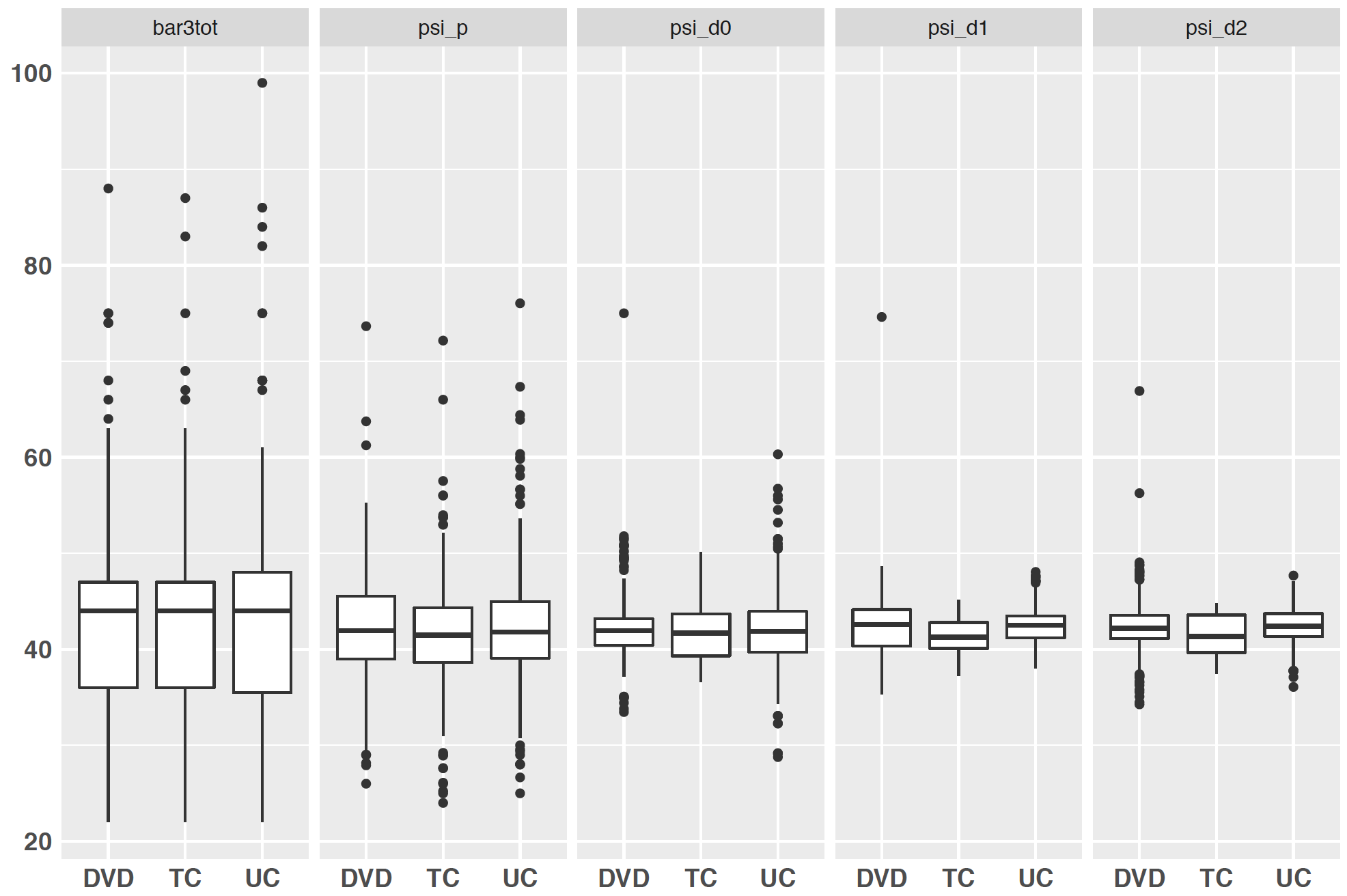
Boxplots of values of and with , or are shown in Figure 2.
It can be seen that clearly without using any covariate has much larger variability than ’s using covariate information, and
has the largest
variability among the four estimators using covariates. For DVD group,
has the least variability but
is not too bad. For TC, is the best. For UC,
and are comparable and are much less variable than .
Note that we can estimate using the average of
’s with ’s in each method group and , or .
Using ’s and 10,000 random permutations, we obtain p-values
for testing various hypotheses based on
, or . The results are shown in Table 4. The reason we also consider one-sided tests is because the method with smaller is better at promoting mammography screening.
Figure 2: Boxplots of and in each method group, , or .
Table 4: p-values using and 10,000 permutations under different hypotheses
method
0.55
0.65
0.49
0.88
0.27
0.68
0.25
0.56
0.04
0.01
0.00
0.00
0.02
0.01
0.00
0.00
0.18
0.00
0.00
0.00
0.09
0.00
0.00
0.00
The results in Table 4 show that TC is better than either UC or DVD with high significance when
,
, or
is used, but not . Thus, applying SDR is beneficial in this example.
Also, all methods cannot detect any difference between DVD and UC.
The previous analysis shows some advantages of using the proposed
and/or , but the accuracy of estimators of has not been
investigated. Different from the simulation study,
the true value of is unknown in the real data analysis. Thus, we apply the following cross-validation to assess the accuracy for different estimation methods.
The following discussion is for a fixed DVD, TC, or UC.
We divide the dataset into 10 subsets with roughly the same sample size, say . Let be one such subset, . We use data not in but in other subsets to obtain the estimator , where supscript indicates using data not in and , or . Then, we assess the accuracy by for , noting that , , are not used in the construction of . After crossover all , we
estimate by
However, is not the mean-squared error of .
Note that
because the cross product term
The term is an average mean squared error (AMSE) of
over all values.
If we can estimate by , then we can estimate AMSE of by .
We utilize the difference-based variance estimators proposed in Hall et al., (1990), Hall et al., (1991) and Munk et al., (2005) to estimate , where in
is
replaced by .
Estimated values of , AMSE for
, ,
and for three groups DVD, TC, and UC are
given in Table 5.
It can be seen from Table 5 that using data helps in the estimation of on the average, especially when we use .
Appendix
Proof of Lemma 1
Proof.
(i) Since , then and further . By the definition of partial central subspace in Chiaromonte et al., (2002),
the partial central space . By Proposition 3.1 and equation (3.1) in Hung et al., (2015), it is easy to get . Furthermore, if , by the denfinition of central subspace in Cook, (1998), .
(ii)
For the same reason as in (i), the partial central space , and then we can get . On the other hand, . As a result, , which means .
∎
The following Lemmas 2 - 6 are all used for the proof of Theorem 1.
Lemma 2.
If
Assumptions
1,
3(i)(ii) and
4 hold, then
and
Proof.
The proof is analogous to that of Lemma 3 in the supplementary materials of Ma and Zhu, (2012).
∎
Making use of the results in Lemma 2, we prove in the following Lemma 3 that the estimation errors of SDR are asymptotically negligible. Note that we assume that SDR estimators of and converge at the rate of .
For the following lemmas and proofs, when necessary, we use to represent based on and , and use to represent based on and .
Also, the denominator of converges to . Hence . As to , by Lipschitz continuity in
Assumption
3(iii),
for some constant , hence . Then . The proof of is similar. As to ,
where by the uniform convergence result from
Lemma 2 and
Assumption
4. As to ,
where . Thus . Therefore, and are both . This completes the proof.
∎
By Lemma 3, the estimation errors of SDR estimators have no effect on the asymptotic distribution of
. Hence, in the following lemmas and proofs, we assume that are known.
The denominator of ,
,
converges in probability to . By Slutsky’s theorem, we only need to prove that the numerator of is asymptotically normal. Write the numerator of in the form of with and . In the following proofs, we distinguish the kernels by denoting and as the kernel functions used in the first and second steps, respectively, and we use , and as generic constants.
The following Lemmas 4 - 6 together prove that
which means that the convergence rate of a two-step estimator is not directly affected by the kernel estimation of the inner layer, but by the kernel estimation of the outer layer.
Lemma 4.
If
Assumptions
1,
2,
3(ii) and
4 hold, then
where
with some functions , .
Proof.
From
Assumption
1, is bounded away from zero. Since converges to uniformly, when is large enough, is also bounded away from zero, i.e. both and . Then by
Assumptions
2,
3(ii) and
4,
By Chebyshev’s inequality, .
∎
Lemma 5.
Let be as defined in
Lemma 4. If
Assumptions
1,
2,
3(ii) (iv) and
4 hold, then
where is the cdf of .
Proof.
Let , then
We only need to prove that
and
are both .
As can be written in such way that
where
, and .
Result from Lemma 8.4 in Newey and McFadden, (1994) concerning V-statistics convergence is applied directly. Lemma 8.4 states that if are i.i.d then
In ,
Note that and may overlap and it is necessary to find out the basis of before calculating the expectation.
Split the columns of and into two parts such that and , where the columns of and (with the smallest possible column dimensions) together form the basis of the space . In this case, the columns of (or ) can be written as linear combinations of the columns of and .
Let and be the column dimensions of and respectively.
As the kernels are bounded from above, then there exists such that
and
. By
Assumptions
1 and
3
(ii),
(iv),
where and .
As to ,
where the first term
Similarly .
In all, by
Assumption
4,
As to , by Chebychev’s Inequality,
Assumptions
1,
3
(ii) and
4, since ,
so .
∎
For the following proof, we denote
and .
Lemma 6.
If
Assumptions
1,
2,
3
(ii) and
4 hold, then
Proof.
Since
can be written as
by Chebyshev’s inequality,
so we only need to prove
and .
By
Assumptions
1,
2,
3
(ii) and
4,
By
Lemmas 4 - 6, , and are all .
It is also easy to prove
As a result,
Follow the similar proof as in Theorem 2.2.2 of Bierens, (1987), when
Assumptions
3
(v) and
4 are satisfied,
and its optimal convergence rate is .
Specifically, when , becomes ,
(6) holds and its optimal convergence rate is ; when and Assumptions
1 -
4 are satisfied with , , replaced by , , respectively, becomes ,
(6) holds with , , replaced by , , respectively and , and its optimal convergence rate is .
∎
References
Bierens, (1987)
Bierens, H. J. (1987).
Kernel estimators of regression functions.
Fifth World Congress Advances in Econometrics, 1:99–144.
Champion et al., (2014)
Champion, V. L., Rawl, S. M., Bourff, S. A., Champion, K. M., Smith, L. G.,
Buchanan, A. H., Fish, L. J., Monahan, P. O., Stump, T. E., Springston,
J. K., and et al. (2014).
Randomized trial of dvd, telephone, and usual care for increasing
mammography adherence.
Journal of Health Psychology, 21(6):916–926.
Chiaromonte et al., (2002)
Chiaromonte, F., Cook, R., and Li, B. (2002).
Sufficient dimensions reduction in regressions with categorical
predictors.
The Annals of Statistics, 30(2):475–497.
Cook, (1998)
Cook, R. D. (1998).
Regression graphics: ideas for studying regressions through
graphics.
Wiley.
Cook and Weisberg, (1991)
Cook, R. D. and Weisberg, S. (1991).
Sliced inverse regression for dimension reduction: Comment.
Journal of the American Statistical Association, 86(414):328.
Dong and Li, (2010)
Dong, Y. and Li, B. (2010).
Dimension reduction for non-elliptically distributed predictors:
second-order methods.
Biometrika, 97(2):279–294.
Escanciano et al., (2014)
Escanciano, J. C., Jacho-Chávez, D. T., and Lewbel, A. (2014).
Uniform convergence of weighted sums of non and semiparametric
residuals for estimation and testing.
Journal of Econometrics, 178:426–443.
Hall et al., (1990)
Hall, P., Kay, J. W., and Titterington, D. M. (1990).
Asymptotically optimal difference-based estimation of variance in
nonparametric regression.
Biometrika, 77(3):521.
Hall et al., (1991)
Hall, P., Kay, J. W., and Titterington, D. M. (1991).
On estimation of noise variance in two-dimensional signal processing.
Advances in Applied Probability, 23(3):476.
Hansen, (2008)
Hansen, B. E. (2008).
Uniform convergence rates for kernel estimation with dependent data.
Econometric Theory, 24(03).
Hung et al., (2015)
Hung, H., Liu, C.-Y., and Lu, H. H.-S. (2015).
Sufficient dimension reduction with additional information.
Biostat Biostatistics, 17(3):405–421.
Li and Wang, (2007)
Li, B. and Wang, S. (2007).
On directional regression for dimension reduction.
Journal of the American Statistical Association,
102(479):997–1008.
Li, (1991)
Li, K.-C. (1991).
Sliced inverse regression for dimension reduction: Rejoinder.
Journal of the American Statistical Association, 86(414):337.
Ma and Zhu, (2012)
Ma, Y. and Zhu, L. (2012).
A semiparametric approach to dimension reduction.
Journal of the American Statistical Association,
107(497):168–179.
Mai and Zou, (2015)
Mai, Q. and Zou, H. (2015).
The fused kolmogorov filter: A nonparametric model-free screening
method.
The Annals of Statistics, 43(4):1471–1497.
Munk et al., (2005)
Munk, A., Bissantz, N., Wagner, T., and Freitag, G. (2005).
On difference-based variance estimation in nonparametric regression
when the covariate is high dimensional.
Journal of the Royal Statistical Society: Series B (Statistical
Methodology), 67(1):19–41.
Nadaraya, (1964)
Nadaraya, E. A. (1964).
On estimating regression.
Theory of Probability & Its Applications, 9(1):141–142.
Newey, (1994)
Newey, W. K. (1994).
Kernel estimation of partial means and a general variance estimator.
Econometric Theory, 10(02):1.
Newey and McFadden, (1994)
Newey, W. K. and McFadden, D. (1994).
Large sample estimation and hypothesis testing.
In Engle, R. F. and McFadden, D., editors, Handbook of
Econometrics, volume 4, pages 2113–2245. Elsvier.
Qian and Murphy, (2011)
Qian, M. and Murphy, S. A. (2011).
Performance guarantees for individualized treatment rules.
The Annals of Statistics, 39(2):1180–1210.
Watson, (1964)
Watson, G. S. (1964).
Smooth regression analysis.
Sankhya: The Indian Journal of Statistics, Series A,
26(4):359–372.
Xia et al., (2002)
Xia, Y., Tong, H., Li, W. K., and Zhu, L.-X. (2002).
An adaptive estimation of dimension reduction space.
Journal of the Royal Statistical Society: Series B (Statistical
Methodology), 64(3):363–410.