The large-$N_{c}$ limit of borelized spectral sum rules and the slope of radial Regge trajectories

The case of vector $\rho$-mesons is canonical for the SVZ sum rules method [4]. Let us apply this method to the radial spectrum (2) in the large-$N_{c}$ limit.

The basic theoretical object is the two-point vector correlator $\Pi(Q^{2})$ in Euclidean space defined by

$$\Pi_{\mu\nu}=(q_{\mu}q_{\nu}-g_{\mu\nu}q^{2})\Pi(Q^{2}),$$

(3)

where $\Pi_{\mu\nu}$ represents the T-product of two vector currents interpolating the neutral $\rho^{0}$-meson,

$$\Pi_{\mu\nu}=i\int d^{4}x\,e^{ipx}\left\langle 0|\text{T}\left\{j_{\mu}(x),j_{\nu}(0)\right\}\right|0\rangle,$$

(4)

$$j_{\mu}=\frac{1}{2}(\bar{u}\gamma_{\mu}u-\bar{d}\gamma_{\mu}d).$$

Here $u$ and $d$ are quark fields, and $q$ is the photon spacelike momentum, $q^{2}=-Q^{2}$. The OPE for $\Pi(Q^{2})$ reads [4],

$$\Pi(Q^{2})=\frac{1}{8\pi^{2}}\left(1+\frac{\alpha_{s}}{\pi}\right)\ln\frac{\mu^{2}}{Q^{2}}+\frac{\langle m_{q}\bar{q}q\rangle}{Q^{4}}+\frac{1}{24Q^{4}}\left\langle\frac{\alpha_{s}}{\pi}\left(G_{\mu\nu}^{a}\right)^{2}\right\rangle-\frac{14}{9}\frac{\pi\alpha_{s}}{Q^{6}}\langle\bar{q}q\rangle^{2},$$

(5)

where $q$ stands for $u$ or $d$ quark, the coefficient in front of the last term is given in the large-$N_{c}$ limit (it differs by the common factor $(N_{c}^{2}-1)/N_{c}^{2}$ from the corresponding coefficient in Refs. [4, 5]), and further $\mathcal{O}(Q^{-8})$ terms are neglected. Applying the Borel transform,

$$L_{M}\Pi(Q^{2})=\lim_{\begin{subarray}{c}Q^{2},n\rightarrow\infty\\ Q^{2}/n=M^{2}\end{subarray}}\frac{1}{(n-1)!}(Q^{2})^{n}\left(-\frac{d}{dQ^{2}}\right)^{n}\Pi(Q^{2}),$$

(6)

to the OPE (5) we get

$$L_{M}\Pi(Q^{2})=\frac{1}{8\pi^{2}}\left(1+\frac{\alpha_{s}}{\pi}\right)+\frac{\langle m_{q}\bar{q}q\rangle}{M^{4}}+\frac{1}{24M^{4}}\left\langle\frac{\alpha_{s}}{\pi}\left(G_{\mu\nu}^{a}\right)^{2}\right\rangle-\frac{7}{9}\frac{\pi\alpha_{s}}{M^{6}}\langle\bar{q}q\rangle^{2}.$$

(7)

The vector correlator $\Pi(Q^{2})$ satisfies a dispersion relation with one subtraction,

$$\Pi(q^{2})=\frac{1}{\pi}\int_{4m_{q}^{2}}^{\infty}ds\frac{\text{Im\,}\Pi(s)}{s-q^{2}+i\varepsilon}+\Pi(0).$$

(8)

In the large-$N_{c}$ limit, the mesons are infinitely narrow and saturate completely the two-point correlators [8],

$$\Pi(q^{2})=\sum_{n}\frac{F^{2}_{n}}{q^{2}-m_{n}^{2}+i\varepsilon},$$

(9)

where the residues are defined by $\langle 0|j_{\mu}|V_{n}\rangle=F_{n}m_{n}\varepsilon_{\mu}$. The experimental information on the electromagnetic decay constants $F_{n}$ of radially excited light vector and axial mesons is poor. The quark-hadron duality requires that $F_{n}$ must be constant for the exactly linear spectrum (or decrease at least exponentially with $n$) [9]. For the sake of simplicity (a minimal number of inputs), we will assume that $F_{n}$ represent just a universal constant in the large-$N_{c}$ limit, $F_{n}=F$. The given assumption will lead to rather reasonable numerical predictions and this is enough for the zero-width approximation. The imaginary part of $\Pi(Q^{2})$ takes then a simple form

$$\text{Im\,}\Pi(q^{2})=\sum_{n}\pi F^{2}\delta(q^{2}-m_{n}^{2}).$$

(10)

The Borel transform of (8) in this case is [4]:

$$L_{M}\Pi(Q^{2})=\frac{1}{\pi M^{2}}\int_{0}^{\infty}e^{-s/M^{2}}\text{Im\,}\Pi(s)ds=\frac{F^{2}}{M^{2}}\sum_{n}e^{-m_{n}^{2}/M^{2}},$$

(11)

where we neglected the $\mathcal{O}(m_{q}^{2})$ contribution. Substituting the linear spectrum (2) and summing up we obtain

$$L_{M}\Pi(Q^{2})=\frac{F^{2}}{M^{2}}\frac{e^{-m_{0}^{2}/M^{2}}}{1-e^{-a/M^{2}}}.$$

(12)

The first sum rule arises from equating the relations (5) and (12),

$$\frac{F^{2}e^{-m_{0}^{2}/M^{2}}}{1-e^{-a/M^{2}}}=\frac{M^{2}}{8\pi^{2}}\left[1+\frac{\alpha_{s}}{\pi}+\frac{8\pi^{2}}{M^{4}}\langle m_{q}\bar{q}q\rangle+\frac{\pi^{2}}{3M^{4}}\left\langle\frac{\alpha_{s}}{\pi}\left(G_{\mu\nu}^{a}\right)^{2}\right\rangle-\frac{56}{9}\frac{\pi^{3}\alpha_{s}}{M^{6}}\langle\bar{q}q\rangle^{2}\right].$$

(13)

Following the prescriptions of SVZ method [4], we can get the second sum rule by taking derivative of Eq. (13) with respect to $1/M^{2}$. The meson mass appears directly in the fraction $-\frac{d(13)}{d(1/M^{2})}/(13)$. The given ”combined” sum rule has the form

$$m_{0}^{2}=M^{2}\frac{h_{0}-\frac{h_{2}}{M^{4}}-\frac{2h_{3}}{M^{6}}}{h_{0}+\frac{h_{1}}{M^{2}}+\frac{h_{2}}{M^{4}}+\frac{h_{3}}{M^{6}}}-\frac{a}{e^{a/M^{2}}-1},$$

(14)

where the condensate terms $h_{i}$ are presented in Table 1. In the same table, we display the corresponding terms $h_{i}$ for the axial and scalar cases [4, 5].

The first term in the r.h.s. of Eq. (14) corresponds to the limit $s_{0}\rightarrow\infty$ in the canonical expressions for the meson masses in the SVZ sum rules [5]. The energy cutoff $s_{0}$ is infinite in our case as we take into account an infinite number of radial excitations. The second term is new and reflects contribution of highly excited states. If we knew the slope $a$ we could find from Eq. (14) the mass of ground state $m_{0}$ making use of the standard stability criterion on the Borel [4]. But we will prefer the opposite procedure: Since $m_{0}$ is usually well known, it is interesting to calculate numerical values of slopes for various radial trajectories.

The simplest scalar correlator is defined by replacing the vector current in (4) by the scalar one $j=\bar{q}q$. The OPE for the scalar correlator reads [5]

$$\Pi_{s}(q^{2})=\frac{3}{8\pi^{2}}\left(1+\frac{11}{3}\frac{\alpha_{s}}{\pi}\right)Q^{2}\ln\frac{Q^{2}}{\mu^{2}}+\frac{3}{Q^{2}}\langle m_{q}\bar{q}q\rangle\\ +\frac{1}{8Q^{2}}\left\langle\frac{\alpha_{s}}{\pi}\left(G_{\mu\nu}^{a}\right)^{2}\right\rangle-\frac{22}{3}\frac{\pi\alpha_{s}}{Q^{4}}\langle\bar{q}q\rangle^{2},$$

(15)

where the coefficient in the last term is written in the large-$N_{c}$ limit. We define the spectral representation as

$$\Pi_{s}(q^{2})=\sum_{n}\frac{G^{2}m_{n}^{2}}{q^{2}-m_{n}^{2}+i\varepsilon}.$$

(16)

Here the constant $G^{2}$ represents a scalar analog of vector residue $F^{2}$. Substituting the linear spectrum (2) and repeating the operations of the previous Section we will arrive at the following ”combined” sum rule in the scalar channel,

$$m_{0}^{4}\left(e^{a/M^{2}}-1\right)+2am_{0}^{2}=\textbf{L}\left(a-m_{0}^{2}+m_{0}^{2}\,e^{a/M^{2}}\right)-a^{2}\frac{e^{a/M^{2}}+1}{e^{a/M^{2}}-1},$$

(17)

where

$$\textbf{L}\equiv M^{2}\frac{2h_{0}+\frac{h_{3}}{M^{6}}}{h_{0}+\frac{h_{2}}{M^{4}}-\frac{h_{3}}{M^{6}}},$$

(18)

and the coefficients $h_{i}$ are given in Table 1. The relation (17) represents a quadratic equation for the intercept $m_{0}^{2}$. The corresponding two solutions are

$$m_{0}^{2}=\frac{a}{1-e^{a/M^{2}}}+\frac{\textbf{L}}{2}\pm\frac{\sqrt{\textbf{L}^{2}\left(e^{a/M^{2}}-1\right)^{2}\!/4-a^{2}e^{a/M^{2}}}}{e^{a/M^{2}}-1}.$$

(19)

Below we will discuss both solutions.

The numerical values of input parameters $h_{i}$ in Table 1 which we will use are displayed in Table 2. Below these numbers are briefly commented.

We set $h_{0}=1$ since taking the perturbative threshold $s_{0}\rightarrow\infty$ (infinite number of radial states) we should formally have $\alpha_{s}\rightarrow 0$ due to the asymptotic freedom. This is tantamount to neglecting the loop corrections to the unit operator in the OPE.

The values of gluon and quark condensates are taken from Ref. [4]: $\left\langle\frac{\alpha_{s}}{\pi}\left(G_{\mu\nu}^{a}\right)^{2}\right\rangle=(330\,\text{MeV})^{4},$ and $\langle\bar{q}q\rangle=-(250\,\text{MeV})^{3}$. The first value is scale-independent while the second one is taken roughly at the scale $\mu=1$ GeV. From the Gell-Mann–Oakes –Renner relation, $m_{\pi}^{2}f_{\pi}^{2}=-(m_{u}+m_{d})\langle\bar{q}q\rangle$, with the pion mass $m_{\pi}=140$ MeV [11] and pion weak decay constant $f_{\pi}=92.4\,\text{MeV}$, one gets $m_{u}+m_{d}\approx 10.7\,\text{MeV}\Bigr|_{\mu=1\,\text{GeV}}$. We consider the isospin limit for the masses of current quarks, $m_{u}=m_{d}\equiv m_{q}$. Thus we get a numerical value for another renormalization invariant condensate of dimension four, $\langle m_{q}\bar{q}q\rangle=-(95.6\,\text{MeV})^{4}$. All these inputs lead to the values of $h_{1}$ and $h_{2}$ in Table 2.

The operator $\alpha_{s}(\bar{q}q)$ has a small anomalous dimension. We will regard the corresponding v.e.v. $\alpha_{s}\langle\bar{q}q\rangle$ as a constant. The condensate $h_{3}$ in the $\rho$-channel is taken from Ref. [4]. All other $h_{3}$ can be then obtained from a rescaling prescribed by the coefficients in the last column of Table 1. Our numerical results, however, will be only slightly dependent on $h_{3}$ or independent of it.

As was mentioned above we will regard $m_{0}$ as the mass of ground state obtained within the classical SVZ sum rules. This reduces the number of input parameters and makes the method more attractive: Fixing the values of condensates in the OPE, one can extract the values of both intercept $m_{0}$ and slope $a$. The first step (extraction of $m_{0}$) is nothing but the standard SVZ sum rule method while the second step represents our extension of this method to the case of infinite linear radial spectrum.

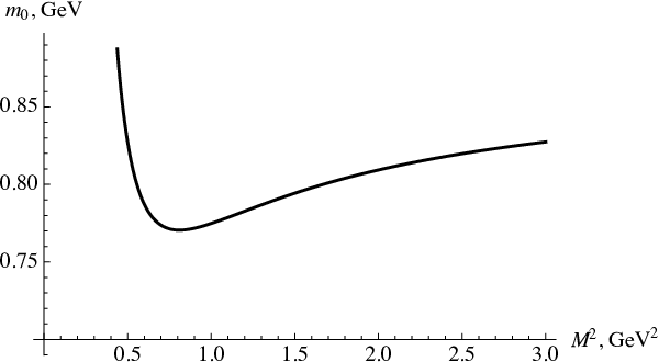
Our strategy is as follows. Consider the $\rho$-meson. We plot $m_{0}$ from Eq. (14) as a function of Borel parameter $M^{2}$ at different values of $a$. A typical plot is presented in Fig. 1. These plots possess the so-called ”Borel window” — a stability region near the minimum where $m_{0}$ is approximately constant. We find the value of $a$ at which $m_{0}$ coincides with the value of $m_{\rho}$ extracted in the usual SVZ sum rules [4, 5]. The obtained $a$ is our prediction for the slope. The slope of $\rho$-trajectory turns out to be near $a_{\rho}=1.52\pm 0.07$ GeV². The predicted masses for this value of slope are presented in Table 3 together with a tentative assignment to experimental data [11]. We give an uncertainty in mass related with uncertainty in extraction of $m_{\rho}$ from the classical SVZ sum rules. The latter uncertainty comes from uncertainty in values of vacuum condensates. In order to avoid double counting of uncertainties we do not use the uncertainties in condensates when calculate $a$. There are of course uncertainties arising from the limits $N_{c}\rightarrow\infty$ and $\alpha_{s}\rightarrow 0$, and from assumed universality of residues. We estimate these uncertainties at the level of 10%.

In the axial-vector case, the stability region exists only at large values of Borel parameter, $M\rightarrow\infty$, see Fig. 2. The same situation takes place within the classical SVZ sum rules [5]. Normalizing our $m_{0}$ to the value $m_{a_{1}}=1.15\pm 0.04$ GeV obtained in Ref. [5], we get $a_{a_{1}}=1.30\pm 0.18$ GeV². The corresponding mass spectrum is presented in Table 4.

Due to the second term in Eq. (14), however, an alternative possibility appears. This additional contribution results in a local maximum in Fig. 2. One can interpret the region near this extremum as an ”emergent” Borel window. The value of $m_{0}$ in this region is surprisingly close to the mass of axial resonance $a_{1}(1260)$ [11] which is traditionally interpreted as an axial partner of $\rho(770)$ if the chiral symmetry were not spontaneously broken. Taking this solution as the ground state we obtain an alternative prediction for the tower of radially excited axial states. The corresponding spectrum is also shown in Table 4.

The scalar case has two solutions (19). The first one (with plus sign) exists at any $M^{2}$ while the second one appears above some positive value of the Borel parameter, see Fig. 3. The first solution corresponds to the value of scalar mass extracted in the classical SVZ sum rules [5]. The stability region lies at $M\rightarrow\infty$ as in the axial case [12]. The standard SVZ method gives $m_{f_{0}}=1.00\pm 0.03$ GeV [5]. Normalizing the first solution to this prediction we obtain $a_{f_{0}}=1.38\pm 0.07$ GeV². If we substitute this value of slope to the second solution we get mass of the ”emerged” lighter scalar meson, $m_{f_{0}}\approx 0.62$ GeV. Our solution predicts thus two parallel scalar trajectories. The ground state on the first trajectory can be identified with $f_{0}(980)$ and on the second one with $f_{0}(500)$ [11]. The existence of two parallel radial scalar trajectories seems to agree with the experimental data [1]. The masses of predicted radial states and a tentative comparison with the observed scalar mesons for two trajectories are displayed in Tables 5 and 6, correspondingly.

References

- [1] A. V. Anisovich, V. V. Anisovich and A. V. Sarantsev, Phys. Rev. D 62, 051502(R) (2000).
- [2] D. V. Bugg, Phys. Rep. 397, 257 (2004); E. Klempt and A. Zaitsev, Phys. Rep. 454, 1 (2007); M. Shifman and A. Vainshtein, Phys. Rev. D 77, 034002 (2008); S. S. Afonin, Eur. Phys. J. A 29, 327 (2006); Phys. Lett. B 639, 258 (2006); Mod. Phys. Lett. A 22, 1359 (2007); Int. J. Mod. Phys. A 22, 4537 (2007); Phys. Rev. C 76, 015202 (2007); P. Masjuan, E. Ruiz Arriola and W. Broniowski, Phys. Rev. D 85, 094006 (2012).
- [3] D. LaCourse and M. G. Olsson, Phys. Rev. D 39, 2751 (1989); A. Yu. Dubin, A. B. Kaidalov and Yu. A. Simonov, Phys. Lett. B 323, 41 (1994); Yu. S. Kalashnikova, A. V. Nefediev and Yu. A. Simonov, Phys. Rev. D 64, 014037 (2001); T. J. Allen, C. Goebel, M. G. Olsson and S. Veseli Phys. Rev. D 64, 094011 (2001); M. Baker and R. Steinke, Phys. Rev. D 65, 094042 (2002); F. Buisseret, Phys. Rev. C 76, 025206 (2007).
- [4] M. A. Shifman, A. I. Vainstein and V. I. Zakharov, Nucl. Phys. B 147, 385, 448 (1979).
- [5] L.J. Reinders, H. Rubinstein, S. Yazaki, 127, 1 (1985).
- [6] P. Colangelo and A. Khodjamirian, hep-ph/0010175.
- [7] G. ’t Hooft, Nucl. Phys. B 72, 461 (1974).
- [8] E. Witten, Nucl. Phys. B 160, 57 (1979).
- [9] M. Shifman, hep-ph/0009131; hep-ph/0507246; S. Beane, Phys. Rev. D 64, 116010 (2001); M. Golterman and S. Peris, JHEP 0101, 028 (2001); Yu. A. Simonov, Phys. Atom. Nucl. 65, 135 (2002); V. A. Andrianov and S. S. Afonin, Phys. Atom. Nucl. 65, 1862 (2002); S. S. Afonin, Phys. Lett. B 576, 122 (2003); Nucl. Phys. B 779, 13 (2007); PMC Phys. A 3, 1 (2009); V. I. Shevchenko and Yu. A. Simonov, Phys. Rev. D 70, 074012 (2004); M. Golterman and S. Peris, Phys. Rev. D 67, 096001 (2003); S. S. Afonin, A. A. Andrianov, V. A. Andrianov and D. Espriu, JHEP 0404, 039 (2004); AIP Conf. Proc. 1030, 177 (2008); O. Cata, M. Golterman and S. Peris, JHEP 0508, 076 (2005); E. R. Arriola and W. Broniowski, Phys. Rev. D 73, 097502 (2006); Eur. Phys. J. A 31, 739 (2007); Phys. Rev. D 81, 054009 (2010); J. J. Sanz-Cillero, Nucl. Phys. B 732, 136 (2006); S. S. Afonin and D. Espriu, JHEP 0609, 047 (2006); J. Mondejar and A. Pineda, JHEP 0710, 061 (2007); A. A. Andrianov and D. Espriu, Phys. Lett. B 671, 275 (2009).
- [10] S. S. Afonin and T. D. Solomko, Eur. Phys. J. C 76, 678 (2016).
- [11] C. Patrignani et al. (Particle Data Group), Chin. Phys. C 40, 100001 (2016).
- [12] S. S. Afonin, Int. J. Mod. Phys. A 31, 1650164 (2016).