Structure formation in clustering DBI dark energy model with constant sound speed
Abstract
Within the framework of DBI non-canonical scalar field model of dark energy, we study the growth of dark matter perturbations in both the linear and non-linear regimes. In our DBI model, we consider the anti-de Sitter warp factor with constant and assume the DBI dark energy to be clustered and its sound speed to be constant. In the linear regime, we use the Pseudo-Newtonian formalism to obtain the growth factor of dark matter perturbations and conclude that for smaller (or ), the growth factor of dark matter is smaller for clustering DBI model compared to the homogeneous one. In the non-linear regime based on the spherical collapse model, we obtain the linear overdensity , the virial overdensity , overdensity at the turn around and the rate of expansion of collapsed region . We point out that for the smaller (or ), the values of , , and in non-clustering DBI models deviate more than the CDM compared to the clustering DBI models. Finally, with the help of spherical collapse parameters we calculate the relative number density of halo objects above a given mass and conclude that the differences between clustering and homogeneous DBI models are more pronounced for the higher-mass halos at high redshift.
Keywords:
cosmological parameters – cosmology: theory – dark energy – large-scale structure of Universe1 Introduction
Observational data from various sources including the type Ia supernovae (SNeIa) (Riess, 1998; Perlmutter, 1999; Kowalski, 2008), cosmic microwave background (CMB) (Komatsu et al., 2009; Jarosik et al., 2011; Komatsu, 2011; Ade et al., 2016), large-scale structure (LSS), baryonic acoustic oscillations (BAO) (Tegmark, 2004; Cole, 2005; Eisenstein, 2005; Percival, 2010; Blake et al., 2011; Reid et al., 2012), high redshift galaxies (Alcaniz, 2004), high redshift galaxy clusters (Wang & Steinhardt, 1998; Allen et al., 2004), and weak gravitational lensing (Benjamin et al., 2007; Amendola et al., 2008; Fu et al., 2008) indicate that our present Universe is in an accelerating phase of expansion. In order to explain this cosmic acceleration in the framework of Einstein’s general relativity (GR), we need to invoke an exotic form of matter-energy with negative pressure, the so-called dark energy (DE). One candidate for the DE is the cosmological constant (Peebles & Ratra, 2003). However, the cosmological constant suffers from fundamental problems such as the fine-tuning and cosmic coincidence problems (Weinberg, 1989; Sahni, 2000; Carroll, 2001; Padmanabhan, 2003; Copeland et al., 2006). Because of these problems, the scientific community suggest dynamical candidates for the DE. The most important class of these models, for example, are the quintessence (Caldwell et al., 1998; Erickson et al., 2002), phantom (Caldwell, 2002; Caldwell et al., 2003; Elizalde, 2004), -essence (Chiba et al., 2000; Armendariz-Picon et al., 2000; Armendariz-Picon et al., 2001), holographic (Horava & Minic, 2000; Thomas, 2002), chaplygin gas (Kamenshchik et al., 2001), generalized chaplygin gas (Bento et al., 2002), dilaton (Gasperini et al., 2001; Arkani-Hamed et al., 2004; Piazza & Tsujikawa, 2004), agegraphic (Cai, 2007), new agegraphic (Wei & Cai, 2008), and quintom (Wei et al., 2005).
Alternatively, the current accelerated expansion of the Universe can be described in the framework of extended theories of gravity, which is so-called modified gravity (MG) (Ida, 2000; Brax et al., 2004; Atazadeh & Sepangi, 2006; Myrzakulov, 2011; Clifton et al., 2012; Guo & Frolov, 2013; Mukherjee & Banerjee, 2014; Cai et al., 2016; Novikov, 2016b; Novikov, 2016a). In the MG models, the gravitational part of the effective action is modified and it is no longer the one related to the Einstein term.
Indeed, the DE (or MG) not only affects the dynamics of the background cosmology through the modification of the Hubble parameter, but also changes the rates of formation and growth of collapsed structures (halos) via its fluctuations. Therefore, in addition to the expansion history, measuring the growth of structure can be used as a useful tool to distinguish between DE (or MG) models. Although different models of DE (or MG) may predict the same background very close to one in the CDM model, they rarely ever create the same perturbations. Thus studying the large-scale structure provides valuable information about the nature of DE (or MG) (Tegmark, 2004; Tegmark et al., 2006). So far, the issue of structure formation in the context of DE models has been extensively considered in the literature (Linder & Jenkins, 2003; Abramo et al., 2007; Sefusatti & Vernizzi, 2011; Batista & Pace, 2013; Roupas et al., 2014; Malekjani et al., 2015; Naderi et al., 2015; Nazari-Pooya et al., 2016; Batista & Marra, 2017; Rezaei et al., 2017; Rezaei & Malekjani, 2017). Also, this subject has been widely studied in the framework of MG theories (Koyama, 2006; Brax & Valageas, 2012; Nesseris, 2013; Asadzadeh et al., 2016; Nunes, 2018).
It is believed that the large-scale structures in the Universe result from the gravitational collapse of primordial small density perturbations (Gunn & Gott, 1972; Press & Schechter, 1974; White & Rees, 1978; Peebles, 1993; Peacock, 1999; Peebles & Ratra, 2003; Ciardi & Ferrara, 2005; Bromm & Yoshida, 2011). The initial seeds of the primordial perturbations are generated during the inflationary phase of our Universe (Guth, 1981; Linde, 1990). At early times of expansion, linear theory of perturbations is valid because the overdensities are small, and also the scales of interest in cosmology are much smaller than the Hubble horizon and the velocities are non-relativistic. Therefore, we can implement the Pseudo-Newtonian gravity that can be used to investigate the evolution of the density fluctuations in the linear regime. In the Pseudo-Newtonian formalism, the relativistic contributions appear as pressure terms in the Poisson equation, and in this way we can use the Newtonian hydrodynamical equations in an expanding Universe (Abramo et al., 2008; Abramo et al., 2009a). It should be noted that at late times the perturbations grow so that the linear regime of perturbations is no longer valid, and we have to examine the evolution of overdensities in the non-linear regime. To this aim, it is convenient to follow the spherical collapse model (SCM) (Gunn & Gott, 1972), which is a simple analytical approach to study the non-linear perturbations. Investigation of the evolution of the fluctuations at this level provides some cosmological results which are observationally valuable. An interesting possibility in the context of SCM is that DE may mutate into a fluid with clustering properties similar to those of dark matter (DM) (Abramo et al., 2008). This effect is a generic feature of DE and originates from a simple idea: when pressure perturbations are large, the effective equation of state inside a collapsed region can be different from the one of its homogeneous component (Abramo et al., 2008). In Abramo et al. (2009a), it has been discussed that the clustering DE can show a detectable impact on the cosmological observables.
Notice that within the framework of canonical scalar fields like the quintessence model (Caldwell et al., 1998; Erickson et al., 2002), the perturbations of DE on small scales of structures are several orders of magnitude smaller than those in the DM and consequently the DE perturbations are usually neglected on these scales. This is because of the fact that the effective sound speed of quintessence perturbations is very close to the light speed () which yields the growth of scalar field perturbations to be suppressed inside the sound horizon. However, in the non-canonical scalar fields like the -essence models (Armendariz-Picon et al., 2000; Chiba et al., 2000; Armendariz-Picon et al., 2001), the DE perturbations can propagate with an effective sound speed much smaller than one and consequently the DE can be clustered in the -essence models on sub-horizon scales.
In this paper, we focus on the study of structure formation in the context of Dirac-Born-Infeld (DBI) scalar field. The DBI scalar field is included in the class of non-canonical scalar fields whose kinetic energy in the action is different from the canonical one. The DBI scalar field has well-based motivations from the string theory. In fact the DBI scalar field is used to describe the dynamics of the radial coordinate of a D3-brane moving in a warped region (throat) of a compactification space (Alishahiha et al., 2004; Silverstein & Tong, 2004). In this description, the brane can be imagined as a point-like object whose speed is limited by the warp factor of the throat. Due to this speed limit, we usually introduce a parameter which is analogous to the Lorentz factor in the special relativity. Note that in the case , the sound speed of the DBI dark energy model is less than the light speed. The sound speed determines the velocity of perturbations propagation among the space, and therefore it is expected this parameter possesses a crucial role in the study of cosmological structure formation. In this paper, our main aim is to investigate the cosmological implications of the clustering () and non-clustering () DBI dark energies with the constant sound speed in both the linear and non-linear regimes of perturbations.
The structure of this paper is as follows. In Sec. 2, we study the background cosmology in the presence of DBI dark energy model. In Sec. 3, we investigate the growth of linear perturbations in this model. In Sec. 4, we study the non-linear evolution of DM and DE fluctuations in the SCM. Finally, Sec. 5 is devoted to our conclusions.
2 Background cosmology in DBI model
In the framework of Einstein gravity, the action of DBI non-canonical scalar field is given by (Silverstein & Tong, 2004)
| (1) |
where , and are the Planck reduced mass, the determinant of the background metric and the Ricci scalar, respectively. Also is the action of matter field and is the Lagrangian density of the DBI scalar field defined as follows
| (2) |
where is the warp factor. Besides, and are the canonical kinetic term and potential of the DBI scalar field , respectively.
The energy density and pressure of the non-canonical scalar field DE corresponding to the DBI Lagrangian (2) take the forms
| (3) | ||||
| (4) |
where the subscript “” denotes the partial derivative with respect to . In addition, the parameter is defined in analogy of the Lorentz boost factor as
| (5) |
which determines the relativistic limit of brane motion in a warped background.
For a spatially flat Friedmann-Robertson-Walker (FRW) Universe containing the DBI dark energy and pressureless DM, variation of the action (1) with respect to the metric reduces to the first and second Friedmann equations as follows
| (6) | ||||
| (7) |
where is the Hubble parameter with the scale factor . Note that for the flat FRW matric, the canonical kinetic term reads .
Taking the variation of action (1) with respect to yields the equation of motion of the scalar field as
| (8) |
where the subscript “” indicates the partial differentiation with respect to . This equation of motion can also be obtained from the continuity equation governing the scalar field
| (9) |
Also the pressureless DM satisfies the following continuity equation
| (10) |
This gives the solution
| (11) |
where is the matter energy density at the present scale factor .
Within the framework of non-canonical scalar field, the sound speed characterizing the propagation speed of the DE fluctuations relative to the homogeneous background is defined as
| (12) |
Note that due to having a real and subluminal sound speed, it should satisfy the condition . Using Eqs. (3) and (4) in (5), the sound speed in DBI dark energy reads
| (13) |
For the case (or ), from Eqs. (3) and (4) we have and consequently our DBI model is transformed to the CDM one.
Note that the set of equations (6), (7), (8) and (10) are not independent of each other. Taking the time derivative of Eq. (6) and using Eqs. (8) and (10), one can obtain the second Friedmann equation (7). In what follows, we take the set of Eqs. (6), (7), and (10), which can uniquely determine the dynamics of the Universe. Now to obtain the evolutionary behaviors of and , we consider the anti-de Sitter (AdS) warp factor with constant and following Spaliński (2008); Tsujikawa et al. (2013); Amani et al. (2018), we assume the sound speed to be constant. Although we assume the sound speed of the DBI dark energy to be constant, this does not confine considerably the generality of our discussion. Since the present Universe experiences an intensive accelerating expansion, following Garriga (1999), we can regard the variation of the sound speed to be much slower than the increase rate of the cosmic scale factor . In spite of the fact that an exact expression has been provided for the sound speed in Eq. (13), but this quantity is slow-varying versus time, and it can be taken as a constant parameter to a good approximation. As we will see, one important consequence of this approximation is that, having the function of the warp factor , we can determine the function of the scalar potential , that we have no robust theoretical or experimental idea for it yet.
Assuming , the set of Eqs. (7) and (13) can be recast in the dimensionless form as
| (14) | ||||
| (15) |
where the prime represents the derivative with respect to the scale factor . Here, we have used and . Also is the dimensionless matter density parameter at the present. Furthermore, for the purpose of numerical computations, it is more convenient to define the following dimensionless variables
Notice that our DBI model described by Eqs. (14) and (15) has four free parameters including , , , and . To investigate the background evolution and the growth of perturbations in our model, we consider two different cases. In the first case, we fix and consider different values of the sound speed . In the second one, we set and choose typical values for the warp parameter as . In the both cases, we fix and at the present time.
Now, we solve Eqs. (14) and (15) numerically with the initial conditions and . With the help of numerical results obtained for and , we can obtain the evolutionary behaviors of the DM and DE density parameters (, ), the deceleration parameter , the equation of state (EoS) parameter of DE , the effective EoS parameter , and the DBI potential . The results are presented in Figs. 1 and 2. The figures show that (i) the DBI model with different and has , which indicates that the Hubble parameter in our model is larger than one in the CDM model. (ii) The density parameters and increase and decrease, respectively, as the redshift decreases. (iii) The deceleration parameter varies from an early matter-dominant epoch to the de Sitter era () in the late-time future, as expected. It also shows a transition from a cosmic deceleration () to an accelerating phase () in the near past. The transition occurs at the redshifts ) for , , ) with (see Fig. 1) and , , for , , ) with (see Fig. 2). The values of in our model are smaller than corresponding to the CDM model. (iv) The EoS parameter of DE, , in our model behaves like the quintessence regime, i.e. . This result is similar to that obtained by Devi & Sen (2011) for the tachyon DE model. (v) The effective EoS parameter, , starts from an early matter-dominated regime () and it behaves like the CDM model () in the late time (). (vi) The DBI scalar field decreases with decreasing the redshift. (vii) The DBI potential for behaves like a nearly flat potential. Using the power-law fitting , we find that for the DBI potential behave as , , and , for , , and , respectively. Here it is important to note that in our DBI model, the slow-roll condition holds because the power-law potentials of our DBI models during the accelerating expansion period of the Universe () behave as flat potentials (see Figs. 1 and 2, the last right panels). Now, according to Garriga (1999) during slow-roll accelerating expansion, the Hubble parameter and the sound speed vary much slower than the scale factor of the Universe. Therefore, we have and . Consequently, in the slow-roll approximation, the assumption of constant sound speed, , is valid. (viii) For smaller (or ), the differences between the DBI model and CDM are more pronounced, while for the DBI model behaves like the CDM one, as expected.


3 Linear perturbation theory
In this section, we study the linear growth rate of density perturbations of non-relativistic DM and DBI dark energy. In the Pseudo-Newtonian (PN) formalism (Hwang & Noh, 1997; Lima et al., 1997; Hwang & Noh, 2006), the linear perturbation equations governing the evolution of non-relativistic dust matter and dark energy density contrasts are given by (Abramo et al., 2009b)
| (16) | ||||
| (17) | ||||
| (18) | ||||
| (19) |
where is the effective sound speed of DE. Also and are the divergence of the comoving peculiar velocities for DM and DE, respectively. On the sub-horizon scales, the Poisson equation in the Fourier space takes the form (Lima et al., 1997)
| (20) |
In order to measure the evolution of DE and DM fluctuations, it is convenient to express Eqs. (16)-(20) in terms of the scale factor , instead of the cosmic time . We reach
| (21) | ||||
| (22) | ||||
| (23) | ||||
| (24) |
where the prime denotes the derivative with respect to , and is the dimensionless form of the parameter. The set of above equations shows that the amount of DE clustering depends on the magnitude of its effective sound speed . For , the DE clusters in a similar manner to DM that we call it full clustering (FCL) DE, and is related to the case which DE is non-clustering (NCL), i.e. . Note that the quantities and are different from each other. The adiabatic sound speed appears in the background cosmology (see Eqs. (14) and (15)), while the effective sound speed only appears when any perturbation of DE is present.
We solve numerically the set of Eqs. (21)-(24) for both the full clustering (, ) and non-clustering (, ) DBI dark energy models, from an initial redshift at the equality epoch till the present time (). We choose the initial conditions of an Einstein-de Sitter (EdS) Universe (Batista & Pace, 2013; Pace et al., 2014b)
| (25) | ||||
| (26) | ||||
| (27) |
which satisfy the set of Eqs. (21)-(24) in the matter-dominated era. With this choice the perturbations remain in the linear regime. Note that in general although during the matter-dominated regime the amplitude of DM perturbations behaves as in which is a constant, and without any loss of generality one can set .
In Figs. 3(a) and 3(b), we plot the evolution of the growth factor, , relative to its value in a pure matter model () versus the redshift for both the NCL and FCL DBI models with different sets of model parameters. The figures imply that (i) for a given , the value of in the CDM model is smaller than one in the DBI model. Also in the limit of , the DBI model behaves like the CDM one. (ii) Similarly to the CDM Universe, in the DBI model, DE suppresses the growth of perturbations at low redshift, and this is due to the fact that at late times DE dominates the energy budget of the Universe. (iii) has a constant behavior at high redshifts, implying that at early times the effects of DE are negligible in all the models. (iv) The growth factor is smaller for clustering DBI model compared to the homogeneous one ().


4 Spherical collapse in the DBI model
Here, we are interested in studying the non-linear evolution of DE and DM fluctuations in the framework of clustering DBI cosmology. The spherical collapse model (SCM) is the simplest analytical tool to study non-linear structure formation (Gunn & Gott, 1972; Padmanabhan, 1993; Fosalba & Gaztanaga, 1998). In the framework of SCM, a single spherically symmetric region with a peculiar expansion rate detaches from the homogeneous background. Due to self-gravity effects, the spherical overdense regions expand more slowly relative to the Hubble flow. This causes the density of the overdense sphere increases compared to the background fluid. Then, at the turnaround redshift, , the spherical region reaches a maximum radius and completely decouples from the background fluid and begins to collapse independently. Eventually, at the virial redshift , the collapsing sphere attains the steady state virial radius. The SCM is based on the crucial assumptions that the density of each component of fluid is always homogeneous in the spherical region (that means it follows the top-hat density profile), and that the velocity profile of each fluid keeps this homogeneity. Notice that in the presence of DE, not only the large-scale gravitational potentials grow slower because of the accelerated expansion of the Universe, but also the dynamical DE can cluster and form halos itself.
The equations governing the dynamical behavior of SCM are as follows (Hu, 1998; Abramo et al., 2009b; Pace et al., 2014b)
| (28) | ||||
| (29) |
where , and are respectively the density contrast, the square of the effective sound speed and the EoS parameter of component . Note that each fluid component obeys a separate equation of the type Eq. (28), while Eq. (29) stands alone and all fluids flow in the same way. This is true because in the SCM a top-hat density profile is used.
In the presence of full clustering DE (), the set of equations (28) and (29) can be written in terms of scale factor as follows
| (30) | ||||
| (31) | ||||
| (32) |
For the case of non-clustering DE (), we only need to solve Eqs. (30) and (32), setting in the latter, and in this case we have the usual SCM for DM (Gunn & Gott, 1972; Padmanabhan, 1993; Percival, 2005).
If we neglect the non-linear terms appeared in Eqs. (30)-(32), we reach the following set of equations for evolution of linear overdensities as
| (33) | ||||
| (34) | ||||
| (35) |
which are the same as Eqs. (21)-(24) in the PN formalism for the case of full clustering DBI dark energy (, ). The non-linear evolution of with/without DBI perturbations with and are shown in Fig. 4(a). The initial conditions are chosen such that the spherical DM structure collapses at the present epoch, i.e. . The figure shows that in the non-clustering DBI model, the DM structures at collapse earlier than those in the clustering DBI models. This means that in our DBI model which has a quintessence () like behavior (see Figs. 1 and 2), the DE overdensities inhibit the growth of DM perturbations. This is in well agreement with that obtained by Abramo et al. (2007) who showed that the inclusion of DE perturbations for the quintessence (, ) and phantom (, ) DE models, respectively, inhibit and enhance the growth of DM perturbations.


In Fig. 4(b), we plot the linear/non-linear perturbations of both the DM and DBI dark energy with and . We see that at early times both the linear and non-linear solutions behave very close to each other and at late times the non-linear solution grows very fast compared to the linear one. This also is in concordance with the result obtained by Abramo et al. (2007) for the clustering DE with non-phantom EoS parameter (i.e. ).
4.1 Spherical collapse parameters
One of the main quantity characterizing the SCM is the critical density contrast or the linear overdensity parameter, . It is defined as in which is the linear matter density contrast computed from Eqs. (33)-(35), with initial conditions such that the non-linear DM overdensity diverges at a given collapse redshift (Pace et al., 2010; Pace et al., 2012; Pace et al., 2014b). Another important quantity in SCM is the virial overdensity defined as . Here is the overdensity at the turn around epoch, is the scale factor normalized to the turn around scale factor and is the ratio between the virialization radius and the turn around radius (Wang & Steinhardt, 1998). In the Einstein-de Sitter (EdS) cosmology, one can easily show that , and which are redshift-independent (Meyer et al., 2012). Note that in the presence of DE, the spherical collapse parameters can change in time. Also the virialization process depends on the DE evolution (Lahav et al., 1991; Maor & Lahav, 2005; Creminelli et al., 2010; Basse et al., 2012).
In Figs. 5 and 6, the evolution of the linear overdensity , the virial overdensity , the overdensity at the turn around and the rate of expansion of collapsed region, (Abramo et al., 2009a) are presented for different sets of model parameters. The figures show that (i) for the case of FCL , DBI perturbations clearly make closer to the CDM compared to the corresponding non-clustering DBI models. This is in well agreement with what found by Pace et al. (2010); Batista & Pace (2013); Pace et al. (2014b); Malekjani et al. (2015). (ii) At high redshifts, the linear overdensity tends to the fiducial value in the EdS Universe. Note that Pace et al. (2017) have shown that the tendency of to the EdS limit at early times strongly depends on the value of the numerical infinity and on the choice of the initial time to start the integration of the equations, . In our numerical calculations to satisfy the EdS limit, following Pace et al. (2017), we set and . (iii) At lower redshifts, where DE dominates, decreases and deviates from the EdS limit. (iv) The virial overdensity in our DBI model at high enough redshift approaches the value in the EdS Universe, i.e. . Because the Universe is dominated by a pressureless dust matter and the effects of DE on structure formation are negligible. For the case of FCL, DE perturbations clearly make closer to the result of the CDM model compared to the corresponding NCL model. These implications are similar to what found by Del Popolo (2006a); Del Popolo (2006b); Pace et al. (2014b); Malekjani et al. (2015). (v) At high redshift, the values of overdensity at turn-around epoch for DBI model asymptotically tends to the value in the EdS Universe . The value of is larger for both the clustering and non-clustering DBI models, compared to the CDM model. At lower redshifts, due to increasing the role of DE, deviates from the EdS limit and the deviation for non-clustering DBI models is smaller than the clustering case. Note that the behaviors of and in our DBI model are similar to those obtained in Devi & Sen (2011) for the tachyon DE model. (vi) The rate of expansion of collapsed region changes its sign from positive to negative value at the turn-around redshift. For with , the transition occurs at the redshifts for non-clustering models and for clustering models. Also for with , the transition occurs at the redshifts in non-clustering models and in clustering models. Note that for CDM, the transition happens at . We can see for non-clustering models, changes its sign faster. It means that for NCL case, turn-around epoch happens sooner compared to clustering DBI model. (vii) Notice that in all the figures, our DBI model in the limit of recovers the results of CDM model.


4.2 Mass function and halo number density
So far, we studied the impact of clustering DBI dark energy on the linear overdensity threshold , the virial overdensity and the overdensity at the turn around . Since we cannot directly observe the process of structure formation, it is convenient to determine a quantity closely related to the observations. This quantity is defined as the comoving number density of virialized structures with masses in the certain range. Using a simple analytical method, Press & Schechter (1974) obtained the abundance of cold DM halos as a function of their mass and a Gaussian distribution function. In the Press-Schechter formalism, the comoving number density of virialized structures with masses in the range and at redshift is given by (Press & Schechter, 1974; Bond, 1991)
| (36) |
where is the background density of matter at the present time, is the rms of the mass fluctuation in spheres of mass , and is the standard mass function. Although the standard mass function works well in estimating the predicted number density of cold DM halos, it fails by predicting too many low-mass and too few high-mass objects (Sheth & Tormen, 1999; Sheth & Tormen, 2002; Lima & Marassi, 2004). Hence, we use a more popular mass function introduced by Sheth and Tormen (ST) (Sheth & Tormen, 1999; Sheth & Tormen, 2002) as follows
| (37) |
where , and . Following Abramo et al. (2007), the quantity can be related to its present value as , where is the linear growth function. Also, is the variance of smoothed linear matter density contrast defined as
| (38) |
where is the scale enclosing the mass , and is a top-hat window function to carry out the smoothing. Also, is the matter power spectrum of density fluctuations given by (Liddle & Lyth, 1993; Liddle et al., 1996)
| (39) |
where (Ade et al., 2016) is the spectral index of primordial perturbation, is the speed of light, and is the present day normalization of the power spectrum. Besides, is the transfer function which depends on cosmological parameters and the nature of the matter in the universe. Here, we use the Bardeen-Bond-Kaiser-Szalay (BBKS) transfer function which is given by (Bardeen et al., 1986),
| (40) |
with where is the shape parameter defined as (Sugiyama, 1995)
| (41) |
Here, is the baryon density parameter, which we take it as (Copi, 1995; Copi et al., 1995). Note that one may use the fitting formulae of Bunn & White (1997) to normalize the power spectrum to the COBE Differential Microwave Radiometer measurment. But here we normalize the power spectrum to the same value today, according to, , where is used to normalize the matter power spectrum of CDM (Ade et al., 2016).
In DE clustering scenario, the perturbations of DE can contribute to the halo mass, thus we must care about its contribution and we should take it into account (Creminelli et al., 2010; Basse et al., 2011; Batista & Pace, 2013; Pace et al., 2014b; Malekjani et al., 2015). The fraction of DE mass to the mass of DM is given by the quantity , where in the case of full clustering DE and top-hat density profile, we have
| (42) |
In Fig. 7, we show the evolution of on the base of Eq. (42) for our DBI model with different and . The figure illustrates that (i) at earlier times, approaches zero. This indicates that the contribution of DE mass to the total mass of halos at high redshifts is negligible. (ii) In the left (right) panel, smaller (smaller ) gives a higher contribution of DE to the total mass of halos. (iii) When , we can see the quantity of tends to zero due to . (iv) For all DBI models studied in this work, is positive. This is because of this fact that for clustering DE models, from the initial condition (26) the evolution of at early times depends on the EoS parameter (Abramo et al., 2007; Pace et al., 2014b). Since our DBI models behave like the quintessence DE () hence we have and consequently from Eq. (42) we obtain .


In the presence of DE contribution to the halo mass which appears in the parameter , Eq. (36) should be corrected as follows (Batista & Pace, 2013; Pace et al., 2014a)
| (43) |
where the halo mass is changed by . It should be noted that the clustering of the DE component can also change the mass function by changing the quantities and . For the homogeneous and clustering DBI dark energy models, respectively, we use Eqs. (36) and (43) to compute the number density of objects above a given mass at fixed redshift as .
In Fig. 8, we show the relative number density of halos above a given mass at different fixed redshifts for both the NCL and FCL DBI models. We see that at (or ), the results of all non-clustering DBI models roughly coincide with (or close to) the CDM model. But for clustering DBI models with smaller values of , the number of objects is more than CDM model. At redshifts and , the number of virialized halos estimated in clustering DBI models is lower than that for homogeneous DBI models. In general, the differences between clustering and homogeneous DBI models with the CDM model are more pronounced at high redshifts and in the high-mass tail of the mass function. This is because of this fact that in the Sheth and Tormen mass function (Sheth & Tormen, 1999; Sheth & Tormen, 2002), the linear overdensity parameter plays an important role. A small variation of has a huge effect on the high-mass tail of the mass function (Batista & Pace, 2013; Pace et al., 2014b; Heneka et al., 2017).
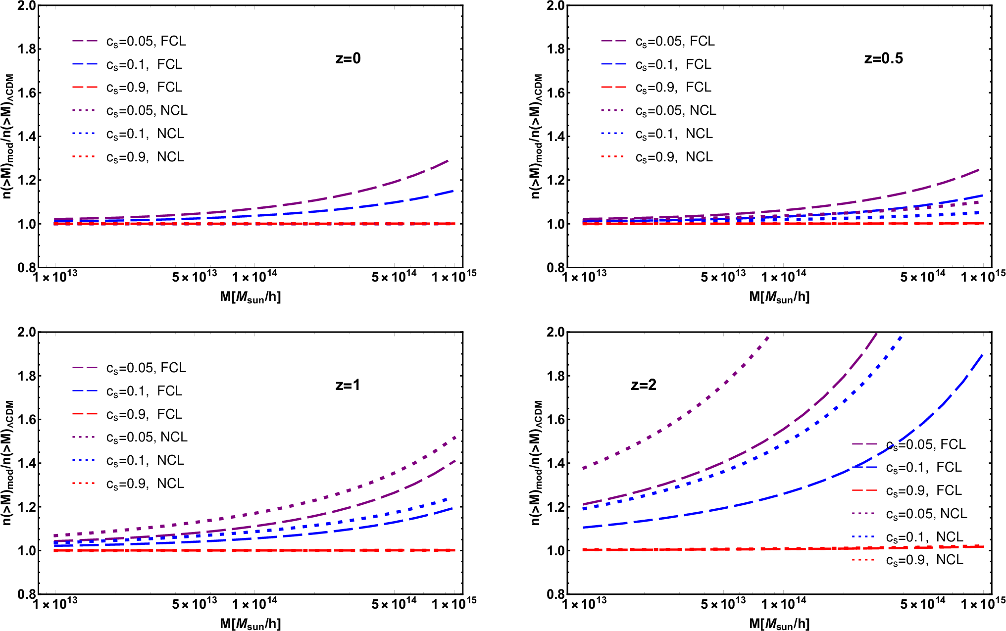
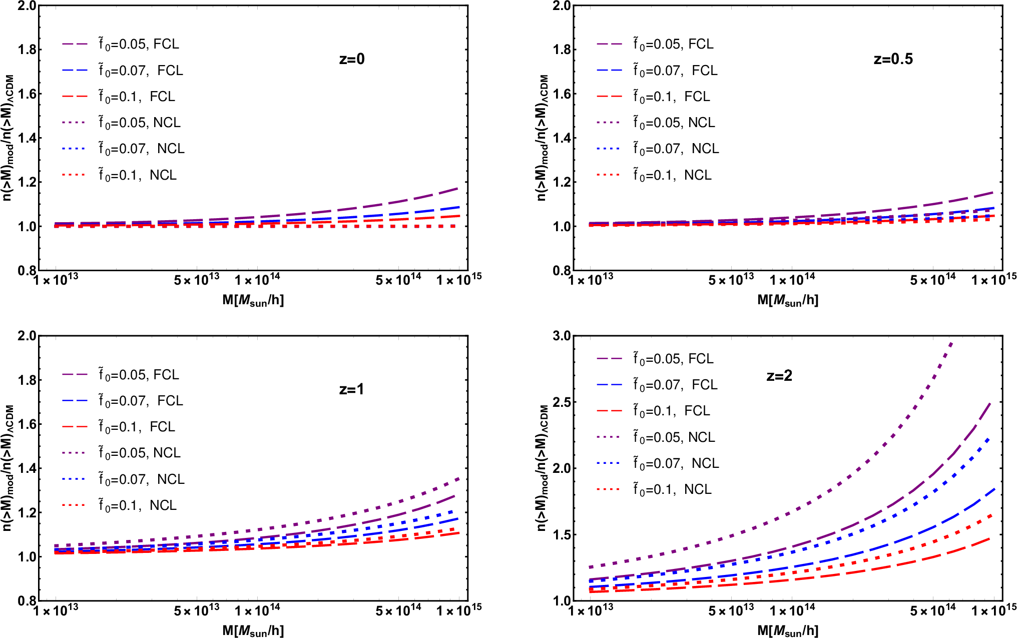
Figure 9 is the same as Fig. 8 but for different values of . The figure clears that for clustering and non-clustering DBI models, the number density is almost equal to or larger than the CDM model. Also similar to Fig. 8, the predicted number of halos in clustering models at lower and higher redshifts, respectively, is more and less than homogeneous DBI models.
5 Conclusions
Here, we studied both the linear and non-linear growth of DM and DE perturbations in the context of DBI non-canonical scalar field. We considered a DBI model with the AdS warp factor and constant sound speed . For the background cosmology, we assumed a spatially flat FRW Universe containing the pressureless DM and DBI dark energy. Then, we investigated the evolution of the background quantities including the Hubble parameter , the density parameters (, ), the deceleration parameter , the DBI and effective EoS parameters (, ) and the DBI scalar field potential . Our results show that (i) for smaller (or ), the background quantities in our DBI model deviate more than those in the CDM model. (ii) behaves like quintessence DE, i.e. . (iii) and vary from matter dominated Universe and approach the de Sitter Universe at late times, as expected. Besides, shows a transition from decelerating () to accelerating () Universe at redshifts close to the CDM model. (iv) For a given and different values of , the DBI potential behaves like the power-law one .
In the linear regime of perturbations based on the PN formalism, we obtained the growth factor, , relative to its value in a pure matter model (). We found that the growth rate of DM in DBI models with smaller (or ) has larger deviations from the CDM model and at the same time these deviations are smaller for clustering models compared to the homogeneous ones.
To study the growth of DM and DBI overdensities, we used the SCM and calculated the linear overdensity , the virial overdensity , the overdensity at the turn around and the rate of expansion of collapsed region . Our results are summarized as follows. (i) For all non-clustering DBI models, the linear overdensity has bigger deviations from CDM model in comparison with clustering DBI models. Also this deviation for DBI models with smaller (or ) is larger than the CDM model. (ii) The virial overdensity and the overdensity at the turn around approach and in high enough redshifts, respectively, which are the same values obtained in the EdS cosmology. This is to be expected, because the impact of DE on the early evolution of the Universe is negligible. In addition, the values of and for the smaller (or ) deviate more than the CDM model. (iii) For larger values of (or ), the rate of expansion of collapsed region is almost similar to the CDM model. Also for the homogeneous DBI models, changes its sign at higher redshifts compared to the clustering ones. This means that for the non-clustering models, the turn-around epochs occur sooner than ones in the clustering DBI models.
Finally, with the help of spherical collapse parameters, we calculated the ratio of DE mass to DM one and the relative number density of objects above a given mass . We found that in the case of , the number density of halos in non-clustering DBI models is very close to the CDM model, but in clustering DBI models with smaller it is bigger than one in the CDM. At redshifts and , the number of virialized halos estimated in clustering models is lower than one in the homogeneous DBI models. In summary, the differences between clustering and homogeneous DBI models are more pronounced at high redshifts and in the high-mass tail of the mass function.
Acknowledgments
The authors thank the anonymous referee for very valuable comments. The work of S. Asadzadeh has been supported financially by Research Institute for Astronomy and Astrophysics of Maragha (RIAAM) under research project No. 1/5440-18.
References
- Abramo et al. (2007) Abramo L. R., Batista R. C., Liberato L., Rosenfeld R., 2007, J. Cosmol. Astropart. Phys., 11, 12
- Abramo et al. (2008) Abramo L. R., Batista R. C., Liberato L., Rosenfeld R., 2008, Phys. Rev. D, 77, 67301
- Abramo et al. (2009a) Abramo L. R., Batista R. C., Rosenfeld R., 2009a, J. Cosmol. Astropart. Phys., 07, 40
- Abramo et al. (2009b) Abramo L. R., Batista R. C., Liberato L., Rosenfeld R., 2009b, Phys. Rev. D, 79, 23516
- Ade et al. (2016) Ade P. A. R., et al., 2016, Astron. Astrophys., 594, A13
- Alcaniz (2004) Alcaniz J. S., 2004, Phys. Rev. D, 69, 83521
- Alishahiha et al. (2004) Alishahiha M., Silverstein E., Tong D., 2004, Phys. Rev. D, 70, 123505
- Allen et al. (2004) Allen S. W., Schmidt R. W., Ebeling H., Fabian A. C., Van Speybroeck L., 2004, Mon. Not. R. Astron. Soc., 353, 457
- Amani et al. (2018) Amani R., Rezazadeh K., Abdolmaleki A., Karami K., 2018, Astrophys. J., 853
- Amendola et al. (2008) Amendola L., Kunz M., Sapone D., 2008, J. Cosmol. Astropart. Phys., 04, 13
- Arkani-Hamed et al. (2004) Arkani-Hamed N., Creminelli P., Mukohyama S., Zaldarriaga M., 2004, J. Cosmol. Astropart. Phys., 04, 1
- Armendariz-Picon et al. (2000) Armendariz-Picon C., Mukhanov V., Steinhardt P. J., 2000, Phys. Rev. Lett., 85, 4438
- Armendariz-Picon et al. (2001) Armendariz-Picon C., Mukhanov V., Steinhardt P. J., 2001, Phys. Rev. D, 63, 103510
- Asadzadeh et al. (2016) Asadzadeh S., Khaledian M. S., Karami K., 2016, Iran. J. Astron. Astrophys., 3, 81
- Atazadeh & Sepangi (2006) Atazadeh K., Sepangi H. R., 2006, Phys. Lett. B, 643, 76
- Bardeen et al. (1986) Bardeen J. M., Bond J. R., Kaiser N., Szalay A. S., 1986, Astrophys. J., 304, 15
- Basse et al. (2011) Basse T., Bjælde O. E., Wong Y. Y. Y., 2011, J. Cosmol. Astropart. Phys., 10, 38
- Basse et al. (2012) Basse T., Bjaelde O. E., Hannestad S., Wong Y. Y. Y., 2012, arXiv:1205.0548
- Batista & Marra (2017) Batista R. C., Marra V., 2017, J. Cosmol. Astropart. Phys., 11, 48
- Batista & Pace (2013) Batista R. C., Pace F., 2013, J. Cosmol. Astropart. Phys., 06, 44
- Benjamin et al. (2007) Benjamin J., et al., 2007, Mon. Not. R. Astron. Soc., 381, 702
- Bento et al. (2002) Bento M. C., Bertolami O., Sen A. A., 2002, Phys. Rev. D, 66, 43507
- Blake et al. (2011) Blake C., et al., 2011, Mon. Not. R. Astron. Soc., 415, 2876
- Bond (1991) Bond J. R., 1991, Astrophys. J., 379, 440
- Brax & Valageas (2012) Brax P., Valageas P., 2012, Phys. Rev. D, 86, 63512
- Brax et al. (2004) Brax P., van de Bruck C., Davis A.-C., 2004, Reports Prog. Phys., 67, 2183
- Bromm & Yoshida (2011) Bromm V., Yoshida N., 2011, Annu. Rev. Astron. Astrophys., 49, 373
- Bunn & White (1997) Bunn E. F., White M., 1997, The Astrophysical Journal, 480, 6
- Cai (2007) Cai R.-G., 2007, Phys. Lett. B, 657, 228
- Cai et al. (2016) Cai Y.-f., Capozziello S., De Laurentis M., Saridakis E. N., 2016, Reports Prog. Phys., 79, 106901
- Caldwell (2002) Caldwell R. R., 2002, Phys. Lett. B, 545, 23
- Caldwell et al. (1998) Caldwell R. R., Dave R., Steinhardt P. J., 1998, Phys. Rev. Lett., 80, 1582
- Caldwell et al. (2003) Caldwell R. R., Kamionkowski M., Weinberg N. N., 2003, Phys. Rev. Lett., 91, 71301
- Carroll (2001) Carroll S. M., 2001, Living Reviews in Relativity, 4, 1
- Chiba et al. (2000) Chiba T., Okabe T., Yamaguchi M., 2000, Phys. Rev. D, 62, 23511
- Ciardi & Ferrara (2005) Ciardi B., Ferrara A., 2005, Space Sci. Rev., 116, 625
- Clifton et al. (2012) Clifton T., Ferreira P. G., Padilla A., Skordis C., 2012, Phys. Rep., 513, 1
- Cole (2005) Cole S., 2005, Mon. Not. R. Astron. Soc., 362, 505
- Copeland et al. (2006) Copeland E. J., Sami M., Tsujikawa S., 2006, Int. J. Mod. Phys. D, 15, 1753
- Copi (1995) Copi C., 1995, Science, 267, 192
- Copi et al. (1995) Copi C. J., Schramm D. N., Turner M. S., 1995, Phys. Rev. Lett., 75, 3981
- Creminelli et al. (2010) Creminelli P., D’Amico G., Norena J., Senatore L., Vernizzi F., 2010, J. Cosmol. Astropart. Phys., 03, 27
- Del Popolo (2006a) Del Popolo A., 2006a, Astron. Astrophys., 448, 439
- Del Popolo (2006b) Del Popolo A., 2006b, Astrophys. J., 637, 12
- Devi & Sen (2011) Devi N. C., Sen A. A., 2011, Mon. Not. R. Astron. Soc., 413, 2371
- Eisenstein (2005) Eisenstein D. J., 2005, Astrophys. J., 633, 560
- Elizalde (2004) Elizalde E., 2004, Phys. Rev. D, 70, 43539
- Erickson et al. (2002) Erickson J. K., Caldwell R. R., Steinhardt P. J., Armendariz-Picon C., Mukhanov V., 2002, Phys. Rev. Lett., 88, 121301
- Fosalba & Gaztanaga (1998) Fosalba P., Gaztanaga E., 1998, Mon. Not. R. Astron. Soc., 301, 503
- Fu et al. (2008) Fu L., et al., 2008, Astron. Astrophys., 479, 9
- Garriga (1999) Garriga J., 1999, Phys. Lett. B, 458, 219
- Gasperini et al. (2001) Gasperini M., Piazza F., Veneziano G., 2001, Phys. Rev. D, 65, 23508
- Gunn & Gott (1972) Gunn J. E., Gott J. R., 1972, Astrophys. J., 176, 1
- Guo & Frolov (2013) Guo J.-Q., Frolov A. V., 2013, Phys. Rev. D, 88, 124036
- Guth (1981) Guth A. H., 1981, Phys. Rev. D, 23, 347
- Heneka et al. (2017) Heneka C., Rapetti D., Cataneo M., Mantz A. B., Allen S. W., von der Linden A., 2017, Mon. Not. R. Astron. Soc., 473, 3882
- Horava & Minic (2000) Horava P., Minic D., 2000, Phys. Rev. Lett., 85, 1610
- Hu (1998) Hu W., 1998, Astrophys. J., 506, 485
- Hwang & Noh (1997) Hwang J.-c., Noh H., 1997, arXiv:astro-ph/9701137
- Hwang & Noh (2006) Hwang J.-c., Noh H., 2006, Gen. Relativ. Gravit., 38, 703
- Ida (2000) Ida D., 2000, J. High Energy Phys., 09, 14
- Jarosik et al. (2011) Jarosik N., et al., 2011, Astrophys. J. Suppl. Ser., 192, 14
- Kamenshchik et al. (2001) Kamenshchik A., Moschella U., Pasquier V., 2001, Phys. Lett. B, 511, 265
- Komatsu (2011) Komatsu E., 2011, Astrophys. J. Suppl. Ser., 192, 18
- Komatsu et al. (2009) Komatsu E., et al., 2009, Astrophys. J. Suppl. Ser., 180, 330
- Kowalski (2008) Kowalski M., 2008, Astrophys. J., 686, 749
- Koyama (2006) Koyama K., 2006, J. Cosmol. Astropart. Phys., 03, 17
- Lahav et al. (1991) Lahav O., Lilje P. B., Primack J. R., Rees M. J., 1991, Mon. Not. R. Astron. Soc., 251, 128
- Liddle & Lyth (1993) Liddle A. R., Lyth D. H., 1993, Phys. Rep., 231, 1
- Liddle et al. (1996) Liddle A. R., Lyth D. H., Viana P. T., White M., 1996, Mon. Not. R. Astron. Soc., 282, 281
- Lima & Marassi (2004) Lima J. A. S., Marassi L., 2004, Int. J. Mod. Phys. D, 13, 1345
- Lima et al. (1997) Lima J. A. S., Zanchin V., Brandenberger R., 1997, Mon. Not. R. Astron. Soc., 291, L1
- Linde (1990) Linde A., 1990, Phys. Lett. B, 238, 160
- Linder & Jenkins (2003) Linder E. V., Jenkins A., 2003, Mon. Not. R. Astron. Soc., 346, 573
- Malekjani et al. (2015) Malekjani M., Naderi T., Pace F., 2015, Mon. Not. R. Astron. Soc., 453, 4148
- Maor & Lahav (2005) Maor I., Lahav O., 2005, J. Cosmol. Astropart. Phys., 07, 3
- Meyer et al. (2012) Meyer S., Pace F., Bartelmann M., 2012, Phys. Rev. D, 86, 103002
- Mukherjee & Banerjee (2014) Mukherjee A., Banerjee N., 2014, Astrophys. Space Sci., 352, 893
- Myrzakulov (2011) Myrzakulov R., 2011, Eur. Phys. J. C, 71, 1752
- Naderi et al. (2015) Naderi T., Malekjani M., Pace F., 2015, Mon. Not. R. Astron. Soc., 447, 1873
- Nazari-Pooya et al. (2016) Nazari-Pooya N., Malekjani M., Pace F., Jassur D. M.-Z., 2016, Mon. Not. R. Astron. Soc., 458, 3795
- Nesseris (2013) Nesseris S., 2013, Phys. Rev. D, 88, 123003
- Novikov (2016a) Novikov E. A., 2016a, Electron. J. Theor. Phys, 13, 35
- Novikov (2016b) Novikov E. A., 2016b, Mod. Phys. Lett. A, 31, 1650092
- Nunes (2018) Nunes R. C., 2018, J. Cosmol. Astropart. Phys., 05, 052
- Pace et al. (2010) Pace F., Waizmann J.-C., Bartelmann M., 2010, Mon. Not. R. Astron. Soc., 406, 1865
- Pace et al. (2012) Pace F., Fedeli C., Moscardini L., Bartelmann M., 2012, Mon. Not. R. Astron. Soc., 422, 1186
- Pace et al. (2014a) Pace F., Moscardini L., Crittenden R., Bartelmann M., Pettorino V., 2014a, Mon. Not. R. Astron. Soc., 437, 547
- Pace et al. (2014b) Pace F., Batista R. C., Del Popolo A., 2014b, Mon. Not. R. Astron. Soc., 445, 648
- Pace et al. (2017) Pace F., Meyer S., Bartelmann M., 2017, J. Cosmol. Astropart. Phys., 10, 040
- Padmanabhan (1993) Padmanabhan T., 1993, Structure formation in the universe. Cambridge university press
- Padmanabhan (2003) Padmanabhan T., 2003, Phys. Rep., 380, 235
- Peacock (1999) Peacock J. A., 1999, Cosmological physics. Cambridge university press
- Peebles (1993) Peebles P. J. E., 1993, Principles of physical cosmology. Princeton University Press
- Peebles & Ratra (2003) Peebles P. J. E., Ratra B., 2003, Rev. Mod. Phys., 75, 559
- Percival (2005) Percival W. J., 2005, Astron. Astrophys., 443, 819
- Percival (2010) Percival W. J., 2010, Mon. Not. R. Astron. Soc., 401, 2148
- Perlmutter (1999) Perlmutter S., 1999, Astrophys. J., 517, 565
- Piazza & Tsujikawa (2004) Piazza F., Tsujikawa S., 2004, J. Cosmol. Astropart. Phys., 07, 4
- Press & Schechter (1974) Press W. H., Schechter P., 1974, Astrophys. J., 187, 425
- Reid et al. (2012) Reid B. A., et al., 2012, Mon. Not. R. Astron. Soc., 426, 2719
- Rezaei & Malekjani (2017) Rezaei M., Malekjani M., 2017, Phys. Rev. D, 96, 63519
- Rezaei et al. (2017) Rezaei M., Malekjani M., Basilakos S., Mehrabi A., Mota D. F., 2017, Astrophys. J., 843, 65
- Riess (1998) Riess A. G., 1998, Astron. J., 116, 1009
- Roupas et al. (2014) Roupas Z., Axenides M., Georgiou G., Saridakis E. N., 2014, Phys. Rev. D, 89, 83002
- Sahni (2000) Sahni V., 2000, Int. J. Mod. Phys. D, 9, 373
- Sefusatti & Vernizzi (2011) Sefusatti E., Vernizzi F., 2011, J. Cosmol. Astropart. Phys., 03, 47
- Sheth & Tormen (1999) Sheth R. K., Tormen G., 1999, Mon. Not. R. Astron. Soc., 308, 119
- Sheth & Tormen (2002) Sheth R. K., Tormen G., 2002, Mon. Not. R. Astron. Soc., 329, 61
- Silverstein & Tong (2004) Silverstein E., Tong D., 2004, Phys. Rev. D, 70, 103505
- Spaliński (2008) Spaliński M., 2008, J. Cosmol. Astropart. Phys., 04, 002
- Sugiyama (1995) Sugiyama N., 1995, ApJS, 100, 281
- Tegmark (2004) Tegmark M., 2004, Phys. Rev. D, 69, 103501
- Tegmark et al. (2006) Tegmark M., et al., 2006, Phys. Rev. D, 74, 123507
- Thomas (2002) Thomas S., 2002, Phys. Rev. Lett., 89, 81301
- Tsujikawa et al. (2013) Tsujikawa S., Ohashi J., Kuroyanagi S., De Felice A., 2013, Phys. Rev. D, 88, 23529
- Wang & Steinhardt (1998) Wang L., Steinhardt P. J., 1998, Astrophys. J., 508, 483
- Wei & Cai (2008) Wei H., Cai R.-G., 2008, Phys. Lett. B, 660, 113
- Wei et al. (2005) Wei H., Cai R.-G., Zeng D.-F., 2005, Class. Quantum Gravity, 22, 3189
- Weinberg (1989) Weinberg S., 1989, Rev. Mod. Phys., 61, 1
- White & Rees (1978) White S. D. M., Rees M. J., 1978, Mon. Not. R. Astron. Soc., 183, 341