Synthetic cooling translational mode of an optically trapped nanoparticle through librational mode

Advancing research progress in quantum optomechanics has attracted people’s a lot interest and paved a way for many applications in the past decade [1, 2, 3]. The optomechanical systems have been applied in many areas, such as generating macroscopic quantum superpositions and entanglement  [4, 5, 6], ultra-sensitive detectors for force [7, 8], quantum information processing [9, 10, 11]. On the ground of different research demands, people studied different optomechanical systems, such as the microtoroid [12], the near-field coupled nano-mechanical oscillators [13], the membrane [14], the superconducting circuits [15], the optical levitated nanoparticles [16, 17] and etc. As a novel optomechanical system, the optically levitated system increasingly attracts people’s attention due to its high mechanical quality factor Q at vacuum (potentially approaching $Q=10^{12}$) and reconfiguration. Such system can be applied to verify the fundamental principle of quantum mechanics [18, 19, 20, 21] and statistical physics [22, 23, 24, 25, 26, 27] and to further investigate nonlinear dynamics [28, 29], precise measurement and etc [30, 31, 32, 33, 34, 35, 36].

The optically levitated systems not only have high mechanical Q, but also have multiple mechanical degrees of freedom, such as translation, rotation and libration. The translational mode can be used to measure the instantaneous velocity of Brownian particle [23, 22], the nanoscale temperature [37], and the magnetic field [38]. The rotation of nanorods and nanoparticles levitated by laser beam also attracts a lot of attentions recently [39]. Circularly polarized trapping laser beam is a well adapted method for particle rotation, and the stable rotation rate of particle can reach up to $5~\rm MHz$ [40] or even $\rm GHz$ [41, 42]. Spatial light modulator based approach [43] and perfect vortex beam with orbital angular momentum [44] also can be utilized for the particle’s rotation. Meanwhile, librational (torsional) mode has been experimentally observed and theoretically explained [45, 46, 47]. The sideband cooing scheme of the torsional mode was also proposed  [47]. This work stimulated a series of works such as the decoherence mechanism of the librational modes [48, 49], and coupling librational modes with the internal spins [50, 51] or the translational degree of freedom [52].

While nonlinearity is ubiquitous and could affect the physical property of optomechanics, the nonlinear optomechanical systems can be used to testify phenomenna of fundamental physics [28, 29, 53], bistability [54, 55, 56], multi-stability [57] and chaos [58, 59]. Many applications of nonlinear optomechanical systems have been reported as well, such as ultrasensitivity optical sensor [60, 61], cooling by utilising nonlinearity [62, 63]. In Ref. [64], the nonlinearity of the optically trapped nanoparticle’s librational mode is studied. It is found that the red detuning driving can induce bistability of librational mode and single mode squeezing can be realised in blue detuning driving.

Stimulated by the previous investigations on the nonlinearity of the librational mode, here we systematically study the nonlinearity of both the librational and the translational modes of a levitated nonspherical nanoparticle, and derive the nonlinear coupling Hamiltonian between the two modes. The librational and translational modes are stable at the same time if and only if the drives on these two mode are both blue-detuning. As long as the red-detuning drive exists, the two motional modes will be bistable or multi-stable. In the steady state regime, the linearized beam-splitter Hamiltonian is derived, and the synthetic cooling of the translational mode by the librational mode is studied [36]. For this synthetic cooling process, the residual air pressure must be matching with effective coupling strength between the librational and translational modes in the effective beam-splitter like Hamiltonian. Besides, the driving amplitudes of these two modes should match each other in order to obtain the optimal sympathetic cooling ratio. Finally, the feedback cooling can improve the sympathetic cooling ratio of translational mode.

This paper is organized as follows: In Section II, we theoretically investigate the effective Hamiltonian and the nonlinearity of librational and translational modes of a nonspheric nanoparticle trapped by laser beams. Consequently, in Section III, we take the stability analysis of this nonlinear system. After that in Section IV, we deduce the Beam Splitter Hamiltonian in steady state regime and present that translational mode can be cooled by librational mode. By utilising feedback cooling, we can increase synthetic cooling ratio of the translational mode. Finally in the last section we present a brief conclusion and a perspective to future studies.

We consider a nanoparticle that is trapped by two strongly focused laser beams that are counter propagating in horizontal direction as shown in Fig.1. The nanoparticle has three translational modes and three librational modes in focal plane [47, 39]. Here, we consider one librational mode and one translational mode of an optically levitated ellipsoidal nanoparticle with long axis $r_{a}$, short axis $r_{b}=r_{c}$ and the density $\rho$.

The potential energy of the ellipsoid in the optical tweezers is [47]:

where $V=4\pi r_{a}r_{b}^{2}/3$ is the volume of the ellipsoid, $c$ is the speed of the light, $\kappa_{x,y}=\alpha_{x,y}/(\epsilon_{0}V)$ are the effective susceptibility of the ellipsoid, $\epsilon_{0}$ is the vacuum permittivity, and $\theta$ is the angle between the long axis($r_{a}$) of the ellipsoid and the electric field of the trapping laser beam. $I_{y}(y)$ is the intensity of trapping laser along y-direction, $I_{0}$ is the center intensity in the focal plane, $I_{0}=\frac{2P_{0}}{\pi\omega_{0}}^{2}$, $P_{0}$ and $\omega_{0}$ are power and waist of the laser respectively.

The particle tend to minimize its potential energy when it is cooled down. Therefore, both the position $y$ and the angle $\theta$ would approach to zero. Here, in order to obtain the high order effects of both the librational and translational modes, we expand potential function to the forth order of both $y$ and $\theta$ around the equilibrium position, $y=0$ and $\theta=0$. The potential becomes

where $U_{0}=-\frac{VI_{0}}{2c}$ and $\kappa_{xy}=\kappa_{x}-\kappa_{y}$. In order to quantize the librational mode and translational mode, we define the following operators

The commutations of them are $[\hat{\theta},\hat{p}_{\theta}]=i\hbar$ and $[\hat{y},\hat{p}_{y}]=i\hbar$. The Hamiltonian of this system $H=T+U(\theta,y)$ can be written as

where $T=I\dot{\theta}^{2}/2$, with $I=4\pi\rho r_{a}r_{b}^{2}(r_{a}^{2}+r_{b}^{2})/15$ being the rotational inertia of the ellipsoid. In this Hamiltonian, the $4\rm{th}$ order nonlinear coefficient are $\eta_{\theta}=\frac{\hbar}{24I}$, $\eta_{y}=\frac{\hbar}{8m\omega_{0}^{2}}$ and $\eta_{\theta y}=\frac{\hbar}{4\omega_{0}I}\sqrt{\frac{(r_{a}^{2}+r_{b}^{2})^{2}\kappa_{xy}}{10\kappa_{x}}}$, the $6\rm{th}$ order nonlinear coefficients are $\eta_{1}=\frac{\hbar^{2}\kappa_{xy}}{16mI\omega_{0}^{2}\kappa_{x}}\sqrt{\frac{c\pi\rho\omega_{0}^{2}(r_{a}^{2}+r_{b}^{2})^{2}}{10\kappa_{xy}P_{0}}}$ and $\eta_{2}=\frac{\hbar^{2}}{48mI}\sqrt{\frac{c\pi\rho}{\kappa_{x}P_{0}}}$ and the $8\rm{th}$ order nonlinear coefficient is $\eta_{3}=\frac{\hbar^{3}c\pi\rho}{192m^{2}I\kappa_{x}P_{0}}$.

As shown in Fig. 2, both the $8\rm{th}$ order and the $6\rm{th}$ order terms are much less than the $4\rm{th}$ order term. Therefore, the $6\rm{th}$ and $8\rm{th}$ order nonlinear terms can be omitted. The Hamiltonian Eq.( II) can be simplified as follow,

Both librational and translational modes can be driven by lasers, whose driving amplitudes and frequencies are respectively $\Omega_{1}$, $\Omega_{2}$, $\omega_{l1}$ and $\omega_{l2}$ for both librational and translational modes [64], the driving Hamiltonian can be described as

In rotating wave frame, the Hamiltonian is transformed following $\hat{H}_{RM}=\hat{U}^{{\dagger}}(\hat{H}_{r}+\hat{H}_{dr})\hat{U}-\hbar\omega_{l1}\hat{b}_{\theta}^{{\dagger}}\hat{b}_{\theta}-\hbar\omega_{l2}\hat{b}_{y}^{{\dagger}}\hat{b}_{y}$ and $\hat{U}=\mathrm{e}^{-\mathrm{i}(\omega_{l1}\hat{b}_{\theta}^{{\dagger}}\hat{b}_{\theta}t+\omega_{l2}\hat{b}_{y}^{{\dagger}}\hat{b}_{y}t)}$, and rotating wave approximation can be utilized for this system. Under the condition $\omega_{l1}\neq\omega_{l2}$, the effective Hamiltonian can be written as

Here we neglect the highly oscillation terms with frequency of $\pm 2\omega_{l1/l2}$ and $\pm 4\omega_{l1/l2}$. $\Delta_{l1/l2}=\omega_{l1/l2}-\omega_{t}^{\theta/y}$. The above Hamiltonian contains the nonlinear terms for both the librational and the translational modes, and the nonlinear coupling between them.

In previous section, we have deduced an effective Hamiltonian (5) for the system with high nonlinearity. The system may show bistable, even multi-stable states other than stable states through the specific drivings. We will study the stable condition through master equation method based on Hamiltonian (5) in this section. The master equation that describes the dynamics of a nanoparticle which couples with the thermal bath [65] is

where $\mathscr{L}_{\theta/y}=\frac{(1+\overline{n}_{\theta/y})}{2}\gamma_{\theta/y}\mathscr{D}_{b_{\theta/y}}+\frac{\overline{n}_{\theta/y}}{2}\gamma_{\theta/y}\mathscr{D}_{b_{\theta/y}^{{\dagger}}}$, with the Lindblad operator $\mathscr{D}_{x}(\rho)=2x\rho x^{{\dagger}}-x^{{\dagger}}x\rho-\rho x^{{\dagger}}x$. Here $\gamma_{\theta/y}$ is the decay rate of librational (translational) mode, and $\overline{n}_{\theta/y}$ is the average phonon number of the librational (translational) thermal reservoir. To investigate the steady state property and the quantum fluctuation of both the librational and the translational modes, the amplitude of the librational mode $\beta_{\theta/y}(t)$ is split into two terms: the average amplitude $\beta_{\theta/y}$ and fluctuation $\delta b_{\theta/y}(t)$. Using the master Eq.( 6), we can deduce that the motional equations for $\beta_{\theta}$ and $\beta_{y}$

Here we apply the semiclassical approximation, and neglect the terms $\left\langle\hat{b}_{\theta/y}^{{\dagger}}\hat{b}_{\theta/y}^{2}\right\rangle-\left\langle\hat{b}_{\theta/y}^{{\dagger}}\right\rangle\left\langle\hat{b}_{\theta/y}^{2}\right\rangle$. Therefore, we have $\left\langle\hat{b}_{\theta/y}^{{\dagger}}\hat{b}_{\theta/y}^{2}\right\rangle=\beta_{\theta/y}^{\ast}\beta_{\theta/y}^{2}$. This approximation requires fluctuation terms $\left\langle(\delta\hat{b}_{\theta/y})^{2}\right\rangle$ and $\left\langle\delta\hat{b}_{\theta/y}^{{\dagger}}\delta\hat{b}_{\theta/y}\right\rangle$ to be much less than $|\beta_{\theta/y}|^{2}$.

To study the steady state more precisely, we derive the equations for the steady state as follows:

where $\tilde{n}_{\theta/y}=|\beta_{\theta/y}|^{2}$ is the average phonon number of the librational (translational) mode and $\Delta_{1/2}=\omega_{t}^{\theta/y}-\omega_{l1/l2}-2\eta_{\theta y}$. Here we set all parameters ($\gamma_{\theta},\gamma_{y},\Delta_{1},\Delta_{2},\eta_{\theta},\eta_{y},\eta_{\theta y},\Omega_{1},\Omega_{2}$) are in units of $\omega_{t}^{\theta}$. The analytical approach to such equations is still under developed, so we study the system through numerical method. In Eq. 8, both detuning $\Delta_{1}$ and $\Delta_{2}$ influence the steady state. Different detuning could give various steady state property. For example, when $\Delta_{1}$ and $\Delta_{2}$ are larger than zero, in another word, where both drives are red detuning, the system presents multi-stability property. As shown in Fig. 3, both $\tilde{n}_{\theta}$ and $\tilde{n}_{y}$ show multi-stability in some parameters region. In this example, we choose an ellipsoidal glass particle with long axis $r_{a}=50~\rm{nm}$ and short axis $r_{b}=25~\rm{nm}$ is trapped by laser, whose power $P=0.1~\rm{W}$ and waist $w=0.6~\mu\rm{m}$, therefore, the oscillating frequency of librational mode and translational mode are respectively $\omega_{t}^{\theta}=2.34~\rm{MHz}$ and $\omega_{t}^{y}=24.5~\rm{kHz}$. The pressure of the residual air $P=10^{-3}~\rm{Pa}$ and the temperature $T=300~\rm{K}$. Hence the damping of librational mode and translational mode, $\gamma_{\theta}=137.2~\rm{Hz}$ and $\gamma_{y}=47~\rm{Hz}$. The nonlinear coefficients, $\eta_{\theta}=0.202~\rm{Hz}$, $\eta_{y}=0.105~\rm{mHz}$ and $\eta_{\theta y}=2.01~\rm{mHz}$. Here we suppose that the driving frequencies are fixed while the driving amplitudes are changeable. The driving frequencies are red detuning and we have taken more examples for investigations of stability in Appendix A. We find that the red detuning drive will make system present bistability even multi-stability. Therefore, we should find the relation between average phonon number of librational mode (translational mode) and driving frequencies in order to find the steady state region of this system under the condition of fixed driving amplitudes.

From the above example, we find that the driving frequencies determine the stability of the librational and translational modes [64]. If the driving amplitudes of both the librational and translational modes are fixed, we can tune the driving frequencies to study the stability of these modes. In this case, we set the drive amplitudes $\Omega_{1}=0.5$ and $\Omega_{2}=0.5$. According to the numerical simulation of Eq.(8), the detunings $\Delta_{1}$ and $\Delta_{2}$ can affect the average phonon number of librational ($n_{\theta}$) and translational ($n_{y}$) modes.

As shown in Fig. 4, if the effective detuning of the librational mode and translational mode are both less than zero, ($\Delta_{1}<0$ and $\Delta_{2}<0$ ), they will both be in steady state. When $\Delta_{2}<0$ and $\Delta_{1}$ is arbitrary, the average phonon number of translational mode will be in steady state. For the rest cases the librational mode and translational mode will not present steady state. In conclusion, the driving frequency determines the stability of librational and translational modes. If both the librational and translational modes are simultaneously in the steady state, the conditions $\Delta_{1}<0$ and $\Delta_{2}<0$ should be satisfied.

Another steady state example for the $\tilde{n}_{\theta}$ and $\tilde{n}_{y}$ is shown in Fig. 5, where both two modes are in the blue detuning drives.

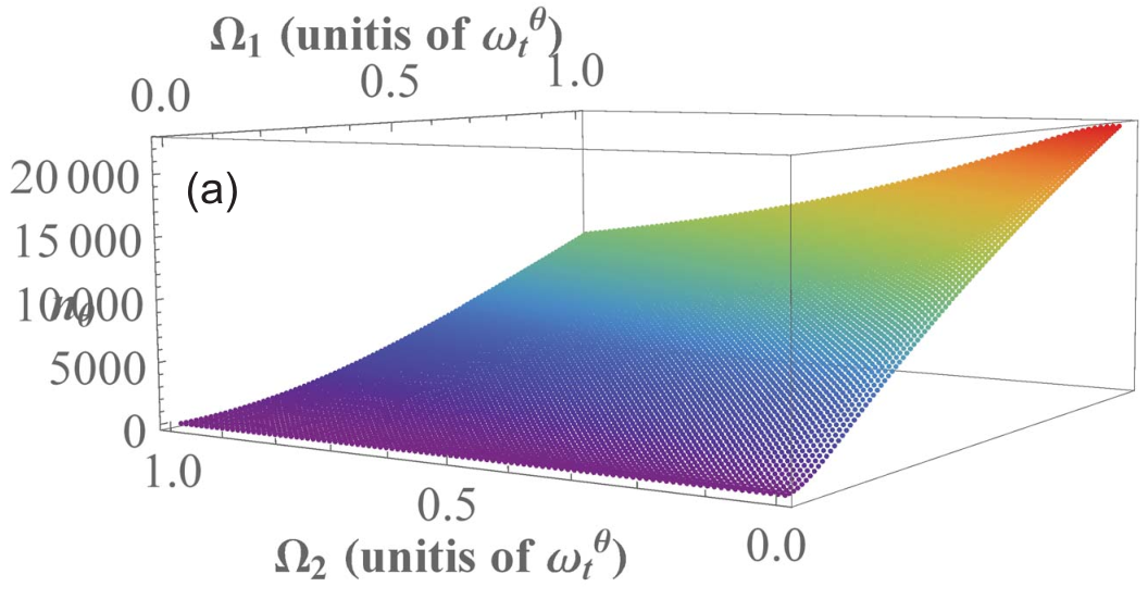
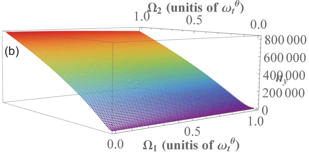
In this case, the average phonon number $\tilde{n}_{\theta}$ and $\tilde{n}_{y}$ can present steady state property in arbitrary drive amplitudes $\Omega_{1}$ and $\Omega_{2}$. This example verifies the conclusion that the coupling bistable system have steady state in blue detuning drivings for arbitrary driving amplitudes.

In summary, $\tilde{n}_{\theta}$ and $\tilde{n}_{y}$ have steady state, bistable state and multistable state in different parameters region shown as above. When one of the drive frequencies $\omega_{l1}$ and $\omega_{l2}$ is red detuning, the average phonon number $\tilde{n}_{\theta}$ and $\tilde{n}_{y}$ will show multi-stability or bistablility in small drive amplitude, however the increment of drive amplitude can make $\tilde{n}_{\theta}$ and $\tilde{y}$ present steady state. It is interesting that when $\omega_{l1}$ and $\omega_{l2}$ are blue detuning, the average phonon number $\tilde{n}_{\theta}$ and $\tilde{n}_{y}$ always present steady state for arbitrary drive amplitude. When the system is in the steady state regime, the driving induced effective coupling between the librational and translational modes can be useful for synthetic cooling.

In the previous section, we discussed the multi-stability of the librational and translational modes, and found the parameter region for the steady states. As we know, the nonlinearity not only stimulates the multi-stability but also induces some novel quantum properties. Here, we discuss another nonlinearity induced phenomena, the synthetic cooling of the translational mode by the librational mode. Through the standard linearization method, we can get the linearized effective Hamiltonian and set $\delta\hat{b}_{\theta/y}\to\hat{b}_{\theta/y}$ for simplicity, and $|\beta_{\theta/y}|\gg 1$, the linearized Hamiltonian reads

where

It is clear that the condition $\Delta_{1}-24\eta_{\theta}|\beta_{\theta}|^{2}-4\eta_{\theta y}(|\beta_{y}|^{2}+1)=\Delta_{2}-24\eta_{y}|\beta_{y}|^{2}-4\eta_{\theta y}(|\beta_{\theta}|^{2}+1)+\delta$ can be satisfied by adjusting the drive frequencies $\omega_{l1}$ and $\omega_{l2}$. For convenience, $\Delta_{{\rm eff}1}=\Delta_{1}-24\eta_{\theta}|\beta_{\theta}|^{2}-4\eta_{\theta y}(|\beta_{y}|^{2}+1)$ and $\Delta_{{\rm eff}}=\Delta_{2}-24\eta_{y}|\beta_{y}|^{2}-4\eta_{\theta y}(|\beta_{\theta}|^{2}+1)$ are fixed, and $\Delta_{{\rm eff}1}-\Delta_{{\rm eff}2}=\delta$. By utilizing the rotating frame Transformation and the rotating wave approximation, Eq.(9) can be transformed into beam-splitter-like Hamiltonian

where $\hat{H}_{\rm{bs}1}=-\hbar\delta\hat{b}_{y}^{{\dagger}}\hat{b}_{y}$, and $\hat{H}_{\rm{bs}2}=-4\hbar\eta_{\theta y}(\beta_{\theta}\beta_{y}^{\ast}\hat{b}_{\theta}^{{\dagger}}\hat{b}_{y}+{\rm H.C.})$.

Based on Hamiltonian (11), the master equation of the system is

where $\mathscr{L}_{\theta}=\frac{\gamma_{\theta}}{2}(1+\bar{n}_{\theta})\mathscr{D}_{\theta}+\frac{\gamma_{\theta}}{2}(\bar{n}_{\theta})\mathscr{D}_{\theta^{{\dagger}}}$, $\mathscr{L}_{y}=\frac{\gamma_{y}}{2}(1+\bar{n}_{y})\mathscr{D}_{y}+\frac{\gamma_{y}}{2}(\bar{n}_{y})\mathscr{D}_{y^{{\dagger}}}$ and $\mathscr{D}_{x}=2x\rho x^{{\dagger}}-x^{{\dagger}}x\rho-\rho x^{{\dagger}}x$ is the Lindblad superoperation for $x$ to be $\theta$ or $y$. $\overline{n}_{\theta}$ and $\overline{n}_{y}$ are the average thermal phonon number of librational and translational mode reservoir, respectively. From Eq.( 12), we can adiabatically eliminated the librational mode to get the reduced master equation for the translational mode, and vise versa. Therefore, we can define two superoperators $\mathscr{L}_{int}$ and $\mathscr{L}_{free}$.

In the weak coupling limit, we get the reduced density matrix $\rho_{y}$ which satisfies

Therefore, we can have

By setting $\tilde{\eta}=\frac{32(\gamma_{\theta}+\gamma_{y})\eta_{\theta y}^{2}|\beta_{\theta}\beta_{y}|^{2}}{(\gamma_{\theta}+\gamma_{y})^{2}+4\delta^{2}}$, we can get the evolution equation of the fluctuation of average phonon number of the translational mode,

And for the librational mode, we can have the similar evolution equation of the fluctuation of average phonon number of the librational mode,

By solving Eq.(16) and (17), we can get the average fluctuations of the steady state phonon number for both translational and librational modes.

For simplicity, we set $\langle\hat{n}_{y}\rangle=n_{y}$ and $\langle\hat{n}_{\theta}\rangle=n_{\theta}$. Because the translational mode and the librational mode are in the same temperature before cooling, the average excitation number $\bar{n}_{\theta}$ of librational mode is much less than the translational mode average excitation number $\bar{n}_{y}$. Therefore, the translational mode can be cooled and the librational mode is heated after synthetic cooling. The cooling ratio $\xi=n_{y}^{\prime}/\overline{n}_{y}$ could be used to qualify the cooling.

As previously mentioned, the translational mode is cooled and the cooling ratio ($\xi$) is determined by the decay of translational and librational mode, $\gamma_{y}$ and $\gamma_{\theta}$. These decays depend on both the residual air pressure ($P$) and the environment temperature $T$. The difference ($\delta$) between $\Delta_{{\rm eff}1}$ and $\Delta_{{\rm eff}2}$, is also important for cooling. The steady state phonon number of both the librational and translational mode ($\tilde{n}_{\theta}$ and $\tilde{n}_{y}$) are controlled by the driving amplitudes ($\Omega_{1}$ and $\Omega_{2}$). Therefore, we should consider the effect of the driving amplitudes for cooling. At first, we fix the driving amplitude ($\Omega_{1}=0.1$ and $\Omega_{2}=0.1$) and the environment temperature ($T=300~K$). The cooling ratio $\xi$ is only determined by residual air pressure($P$) and $\delta$, as shown like Fig. 6.

The numerical solution presents that the higher vacuum is better for cooling. Nevertheless, when the residual air pressure is higher than $10^{-5}~Pa$, the cooling ratio is saturated. The optimal cooling takes place when the effective detuning $\Delta_{{\rm eff}1}$ and $\Delta_{{\rm eff}2}$ match each other perfectly.

Driving amplitudes, $\Omega_{1}$ and $\Omega_{2}$, can affect the steady phonon number $\tilde{n}_{\theta}$ and $\tilde{n}_{y}$, the driving amplitudes also affect the cooling ratio $\xi$. Taking Fig. 7 (a) for and example, when the driving amplitude of librational mode is fixed, the increment of $\Omega_{2}$ is good for cooling. $\Omega_{1}$ also plays part in this process. When $\Omega_{1}$ is small, although increment $\Omega_{2}$ is good for cooling, the cooling ratio will reach limit and trend to constant when $\Omega_{2}$ is larger than $0.01$, for example $\Omega_{1}=0.05$ in Fig. 7(a). Similar phenomenon also happens when $\Omega_{1}$ is changing for fixed $\Omega_{2}$, for example $\Omega_{2}=0.01$ in Fig. 7(b).

Therefore, the driving amplitude of these two mode should cooperate for cooling. When the driving amplitude increases, the cooling ratio will gradually saturates shown as the dashed and doted dashed lines in Fig. 7. When $\Omega_{1}$ or $\Omega_{2}$ are fixed and optimized for cooling, the increment of $\Omega_{2}$ or $\Omega_{1}$ cannot remarkably strengthen cooling effect. Fig. 7 shows that the cooling ratio is $\xi=0.57$.

In order to get higher cooling effect, the feedback cooling can be used. When the cooling ratio of the translational mode saturates, the feedback cooling scheme can improve the cooling ratio further. The fluctuation of steady state phonon number of translational mode after feedback cooling reads

where $n_{y}^{\prime}$ is the fluctuation of steady state phonon number of the translational mode under the feedback cooling and $\tilde{n}^{\prime}_{\theta/y}$ is the steady state phonon number of librational mode or translational mode. In this scheme, the residual air pressure $P$ and environment ($T$) are fixed, the decays of librational and translational mode do not change. By increasing the feedback strength, the synthetic cooling ratio can be promoted further for the fixed driving amplitudes. Meanwhile, because driving amplitudes directly affect the steady state average phonon numbers, $\tilde{n}^{\prime}_{\theta}$ and $\tilde{n}^{\prime}_{y}$, the synthetic cooling ratio is also determined by driving amplitudes of the translational and librational modes. For depicting more clearly, the decay caused by feedback $\gamma_{\rm fb}$ can be in units of $\gamma_{\theta}$.

As shown in Fig. 7, the synthetic cooling of translational mode will saturate when the driving amplitudes increase. The feedback cooling scheme can break through the saturation of synthetic cooling and promote the cooling ratio in Fig. 8. Because driving amplitudes is also an important aspect for the synthetic cooling of translational mode, $\Omega_{1}$ and $\Omega_{2}$ will affect the cooling ratio. When $\Omega_{1}$ and $\Omega_{2}$ do not match each other, the synthetic cooling ratio will not be significantly promoted and even the translational mode will be heated with the increment of feedback strength. For example, the red-dashed line in Fig. 8. And when the driving amplitudes match each other, the synthetic cooling ratio can be significantly improved and even reaches one percent of the ambient temperature shown as blue line in Fig. 8. In a word, feedback cooling can effectively improve the synthetic cooling ratio when driving amplitudes match each other or else feedback cooling will heat the translational mode.

In the last section, the beam-splitter Hamiltonian was obtained by adjusting the driving frequency for the cooling of translational mode. And when $\Delta_{1}-24\eta_{\theta}|\beta_{\theta}|^{2}-4\eta_{\theta y}(|\beta_{y}|^{2}+1)=-\big(\Delta_{2}-24\eta_{y}|\beta_{y}|^{2}-4\eta_{\theta y}(|\beta_{\theta}|^{2}+1)\big)+\varphi$ with constant $\varphi$, the linearised Hamiltonian Eq.(9) can be transformed to the two-modes squeezing Hamiltonian as follow:

In this way, the two-mode squeezing between the librational and the translational modes can also be generated, similarly as the Ref.  [66, 67, 68].

In this paper we systematically studied the coupling nonlinearity between librational mode and translational mode of an optically levitated ellipsoidal nanoparticle. The coupling of librational mode and translational mode is small, but it should not be neglected when proper driving is applied. For coupling the Hamiltonian of these two motive modes, the stable-state analysis shows the driven librational mode and translational mode could have coupling bistability and one red-detuning drive of any mode could also stimulate the bistablity of other mode. In order to stabilize the system, the drives on the librational and the translational modes should be both blue-detuned. For the linearized coupling Hamiltonian between librational mode and translational mode, the synthetic cooling can be realised in steady state regime. To cool the translational mode by the librational mode, the lower pressure of air residual is always not helpful to translational mode cooling, and the cooling efficiency can be saturated when pressure decreases. The driving amplitude of these two modes is also important for sympathetic cooling, and the driving amplitude matching each other can increase the cooling efficiency of translational mode. However, here the cooling ratio is only $0.57$ of the initial temperature. To solve the problem we used the feedback cooling about librational mode for cooling the translational mode. This scheme breaks through the cooling ratio and improves the cooling efficient remarkably, and even reaches one percent of the ambient temperature. These investigations give us a new platform for the preparing macroscopic ground state, quantum information processing, etc.

References

- [1] T. Kippenberg and K. Vahala, Opt. Express 15, 17172 (2007).
- [2] Y.-C. Liu, Y.-W. Hu, W. Wong Chee, and Y.-F. Xiao, Chinese Physics B 22, 114213 (2013).
- [3] M. Aspelmeyer, T. J. Kippenberg, and F. Marquardt, Rev. Mod. Phys. 86, 1391 (2014).
- [4] A. D. O¡¯Connell, M. Hofheinz, M. Ansmann, R. C. Bialczak, M. Lenander, E. Lucero, M. Neeley, D. Sank, H. Wang, M. Weides, et al., Nature 464, 697 (2010).
- [5] Y. Chen, Journal of Physics B: Atomic, Molecular and Optical Physics 46, 104001 (2013).
- [6] M. Wang, X.-Y. Lü, Y.-D. Wang, J. Q. You, and Y. Wu, Phys. Rev. A 94, 053807 (2016).
- [7] G. Ranjit, D. P. Atherton, J. H. Stutz, M. Cunningham, and A. A. Geraci, Phys. Rev. A 91, 051805 (2015).
- [8] G. Ranjit, M. Cunningham, K. Casey, and A. A. Geraci, Phys. Rev. A 93, 053801 (2016).
- [9] R. W. Andrews, R. W. Peterson, T. P. Purdy, K. Cicak, R. W. Simmonds, C. A. Regal, and K. W. Lehnert, Nature Physics 10, 321 (2014).
- [10] Z.-q. Yin, W. L. Yang, L. Sun, and L. M. Duan, Phys. Rev. A 91, 012333 (2015).
- [11] A. Reed, K. Mayer, J. Teufel, L. Burkhart, W. Pfaff, M. Reagor, L. Sletten, X. Ma, R. Schoelkopf, E. Knill, et al., Nature Physics 13, 1163 (2017).
- [12] A. Schliesser, O. Arcizet, R. Rivière, G. Anetsberger, and T. J. Kippenberg, Nature Physics 5, 509 (2009).
- [13] G. Anetsberger, O. Arcizet, Q. P. Unterreithmeier, R. Rivière, A. Schliesser, E. M. Weig, J. P. Kotthaus, and T. J. Kippenberg, Nature Physics 5, 909 (2009).
- [14] J. Thompson, B. Zwickl, A. Jayich, F. Marquardt, S. Girvin, and J. Harris, Nature 452, 72 (2008).
- [15] J. Teufel, T. Donner, D. Li, J. Harlow, M. Allman, K. Cicak, A. Sirois, J. D. Whittaker, K. Lehnert, and R. W. Simmonds, Nature 475, 359 (2011).
- [16] Z.-q. Yin, A. A. Geraci, and T. Li, International Journal of Modern Physics B 27, 1330018 (2013).
- [17] L. P. Neukirch and A. N. Vamivakas, Contemporary Physics 56, 48 (2015).
- [18] O. Romero-Isart, M. L. Juan, R. Quidant, and J. I. Cirac, New J. Phys. 12, 033015 (2010).
- [19] D. E. Chang, C. A. Regal, S. B. Papp, D. J. Wilson, J. Ye, O. Painter, H. J. Kimble, and P. Zoller, Proc.Natl.Acad.Sci.U.S.A. 107, 1005 (2010).
- [20] O. Romero-Isart, A. C. Pflanzer, F. Blaser, R. Kaltenbaek, N. Kiesel, M. Aspelmeyer, and J. I. Cirac, Phys. Rev. Lett. 107, 020405 (2011).
- [21] Z.-q. Yin and T. Li, Contemporary Physics 58, 119 (2017).
- [22] T. Li, S. Kheifets, D. Medellin, and M. G. Raizen, Science 328, 1673 (2010).
- [23] S. Kheifets, A. Simha, K. Melin, T. Li, and M. G. Raizen, Science 343, 1493 (2014).
- [24] J. Gieseler, R. Quidant, C. Dellago, and L. Novotny, Nature Nanotechnology 9, 358 (2014a).
- [25] J. Millen, T. Deesuwan, P. Barker, and J. Anders, Nature Nanotechnology 9, 425 (2014a).
- [26] L. Rondin, J. Gieseler, F. Ricci, R. Quidant, C. Dellago, and L. Novotny, Nature Nanotechnology 12, 1130 (2017).
- [27] T. M. Hoang, R. Pan, J. Ahn, J. Bang, H. T. Quan, and T. Li, Phys. Rev. Lett. 120, 080602 (2018).
- [28] J. Gieseler, L. Novotny, and R. Quidant, Nature Physics 9, 806 (2013).
- [29] J. Gieseler, M. Spasenović, L. Novotny, and R. Quidant, Phys. Rev. Lett. 112, 103603 (2014b).
- [30] A. A. Geraci, S. B. Papp, and J. Kitching, Phys. Rev. Lett. 105, 101101 (2010).
- [31] T. Li, S. Kheifets, and G. Raizen, Mark, Nature Physics 7, 527 (2011).
- [32] Z.-q. Yin, T. Li, and M. Feng, Phys. Rev. A 83, 013816 (2011).
- [33] N. Zhao and Z.-q. Yin, Physical Review A 90, 042118 (2014).
- [34] D. C. Moore, A. D. Rider, and G. Gratta, Phys. Rev. Lett. 113, 251801 (2014).
- [35] M. Rashid, T. Tufarelli, J. Bateman, J. Vovrosh, D. Hempston, M. S. Kim, and H. Ulbricht, Phys. Rev. Lett. 117, 273601 (2016).
- [36] M. Frimmer, J. Gieseler, and L. Novotny, Phys. Rev. Lett. 117, 163601 (2016), URL https://link.aps.org/doi/10.1103/PhysRevLett.117.163601.
- [37] J. Millen, T. Deesuwan, P. Barker, and J. Anders, Nature Nanotechnology 9, 425 (2014b).
- [38] P. Kumar and M. Bhattacharya, Opt. Express 25, 19568 (2017).
- [39] S. Kuhn, A. Kosloff, B. A. Stickler, F. Patolsky, K. Hornberger, M. Arndt, and J. Millen, Optica 4, 356 (2017).
- [40] Y. Arita, M. Mazilu, and K. Dholakia, Nature Communications 4, 2374 (2013).
- [41] R. René, D. Michael, H. Erik, D. Rozenn, F. Martin, W. Dominik, T. Felix, and L. Novotny, ArXiv e-prints (2018), eprint 1803.11160.
- [42] J. Ahn, Z. Xu, J. Bang, Y.-H. Deng, T. M. Hoang, Q. Han, R.-M. Ma, and T. Li, ArXiv e-prints (2018), eprint 1804.06570.
- [43] Y. Arita, M. Mazilu, T. Vettenburg, E. M. Wright, and K. Dholakia, Optics letters 40, 4751 (2015).
- [44] Y. Arita, M. Chen, E. M. Wright, and K. Dholakia, JOSA B 34, C14 (2017).
- [45] G. Volpe and D. Petrov, Phys. Rev. Lett. 97, 210603 (2006).
- [46] F. Pedaci, Z. Huang, M. van, Oene, S. Barland, and H. N. Dekker, Nature Physics 7, 259 (2010).
- [47] T. M. Hoang, Y. Ma, J. Ahn, J. Bang, F. Robicheaux, Z.-Q. Yin, and T. Li, Phys. Rev. Lett. 117, 123604 (2016).
- [48] C. Zhong and F. Robicheaux, Phys. Rev. A 94, 052109 (2016).
- [49] B. A. Stickler, B. Papendell, and K. Hornberger, Phys. Rev. A 94, 033828 (2016).
- [50] Y. Ma, T. M. Hoang, M. Gong, T. Li, and Z.-q. Yin, Phys. Rev. A 96, 023827 (2017).
- [51] T. Delord, L. Nicolas, Y. Chassagneux, and G. Hétet, Phys. Rev. A 96, 063810 (2017).
- [52] S. Liu, T. Li, and Z.-q. Yin, JOSA B 34, C8 (2017).
- [53] X.-Y. Lü, J.-Q. Liao, L. Tian, and F. Nori, Phys. Rev. A 91, 013834 (2015).
- [54] O. Kyriienko, T. C. H. Liew, and I. A. Shelykh, Physical review letters 112, 076402 (2014).
- [55] W. Ge, B. Rodenburg, and M. Bhattacharya, Phys. Rev. A 94, 023808 (2016).
- [56] C. Jiang, X. Bian, Y. Cui, and G. Chen, JOSA B 33, 2099 (2016).
- [57] Y. Chang, T. Shi, Y.-x. Liu, C. Sun, and F. Nori, Physical Review A 83, 063826 (2011).
- [58] L. Bakemeier, A. Alvermann, and H. Fehske, Physical review letters 114, 013601 (2015).
- [59] F. Monifi, J. Zhang, Ş. K. Özdemir, B. Peng, Y.-x. Liu, F. Bo, F. Nori, and L. Yang, Nature Photonics 10, 399 (2016).
- [60] J. Fan, C. Huang, and L. Zhu, Opt. Express 23, 2973 (2015).
- [61] G. Brawley, M. Vanner, P. E. Larsen, S. Schmid, A. Boisen, and W. Bowen, Nature Communications 7, 10988 (2016).
- [62] P. Z. G. Fonseca, E. B. Aranas, J. Millen, T. S. Monteiro, and P. F. Barker, Phys. Rev. Lett. 117, 173602 (2016).
- [63] W.-Z. Zhang, W.-L. Li, J. Cheng, and Q. Mu, arXiv preprint arXiv:1710.11308 (2017).
- [64] K.-W. Xiao, N. Zhao, and Z.-q. Yin, Physical Review A 96, 013837 (2017).
- [65] W. H. Louisell and W. H. Louisell, Quantum statistical properties of radiation, vol. 7 (Wiley New York, 1973).
- [66] H. Tan, G. Li, and P. Meystre, Physical Review A 87, 033829 (2013).
- [67] A. Pontin, M. Bonaldi, A. Borrielli, L. Marconi, F. Marino, G. Pandraud, G. Prodi, P. Sarro, E. Serra, and F. Marin, Physical review letters 116, 103601 (2016).
- [68] K. Cai, R. Wang, Z. Yin, and G. Long, Science China Physics, Mechanics & Astronomy 60, 070311 (2017).