跳到论文正文
W Papers独立论文阅读器 arXiv:1805.02199 论文正文 计算阅读时间 · 0%
引用这篇论文根据当前论文元数据生成,正式投稿前建议核对。


License: arXiv.org perpetual non-exclusive license
arXiv:1805.02199v2 [eess.SP] 22 Jan 2019

Multi-layer Superimposed Transmission with Symbol Boundary Offset for Optical Wireless Scattering Communication

Guanchu Wang    Chen Gong    Zhimeng Jiang    Zhengyuan Xu ††thanks: This work was supported by Key Program of National Natural Science Foundation of China (Grant No. 61631018) and Key Research Program of Frontier Sciences of CAS (Grant No. QYZDY-SSW-JSC003).††thanks: The authors are with Key Laboratory of Wireless-Optical Communications, Chinese Academy of Sciences, School of Information Science and Technology, University of Science and Technology of China, Hefei, China. Email: {hegsns, zhimengj}@mail.ustc.edu.cn, {cgong821, xuzy}@ustc.edu.cn.
Abstract

We investigate the multi-layer superimposed transmission for optical wireless scattering communication where the symbol boundaries on different signal layers are not necessarily aligned in the time domain. We characterize the multi-layer transmission based on a hidden markov model. Then, we obtain the achievable rates of all signal layers and a single layer, and provide a numerical solution. Furthermore, we propose approaches on the channel estimation as well as joint symbol detection and decoding. Finally, both simulations and experiments are conducted to evaluate the performance of the proposed approaches, and validate the feasibility of the proposed transmission and signal detection approaches.

Index Terms: 
NLOS scattering communication, superimposed transmission, hidden markov model, achievable rate, joint detection and decoding.

I Introduction

Non-line of sight (NLOS) Ultra-violet (UV) scattering communication serves as a good candidate for the applications where radio-silence is required and the transmitter-receiver alignment is hard to guarantee due to obstacles or the user mobility. Moreover, it is promising for outdoor communication under strong solar background because of negligible solar radiation in the UV spectrum [1]. Theoretical analysis [2], numerical simulation [3] and real experiments [4, 5] show an extremely large path loss between the transmitter and receiver, where the received signal can be detected by photon-counting receiver and characterized by Poisson distributed number of discrete photoelectrons.

The capacity of point-to-point continuous-time Poisson channel has been investigated in [6, 7, 8] and the capacity of discrete-time Poisson channel has been derived in [9, 10]. Based on the Poisson channel model, several types of channel model such as Poisson fading [11], MIMO [12], interfering [13], broadcast [14] , and multiple access [15, 16, 17] channels have been studied in recent years. Specifically, code-division and non-orthogonal multiple transmission has been studied in [18], and random access packet-switched systems was proposed in [19]. Other existing works on NLOS UV scattering communication based on the Poisson and extended channel model are the channel link gain with impulse response [20, 21], channel estimation with inter-symbol interference [22], signal detection with receiver diversity [23], and the relay protocol [24].

In this work, we characterize multi-layer superimposed transmission in discrete Poisson channel, where the transmitted symbols in various layers are superimposed, and the symbol boundaries on different signal layers are not necessarily aligned. Specifically, we adopt hidden markov model (HMM) [25, 26] to characterize the superimposed channel. Then, we conceive the achievable transmission rates for all signal layers and a single layer, and obtain the exact and approximated solution[27]. For receiver-side signal processing, we propose channel estimation based on expectation-maximization (EM) algorithm [28, 29], and adopt Viterbi [30] and Bahl-Cocke-Jelinek-Raviv (BCJR) [31] algorithms for symbol detection. Furthermore, we propose iterative algorithm for maximum-likelihood/maximum a posteriori probability (ML/MAP) joint decoding [32, 33]. Finally, we conduct offline experiments to evaluate the performance of the proposed approaches. It is seen that based on the experimental measurements, the proposed approaches perform close to the simulation results with identical channel parameters.

The remainder of the paper is organized as follows. In Section II, we characterize the superimposed NLOS scattering communication using HMM. In Section III, we investigate the achievable transmission rates and obtain a numerical solution on the achievable transmission rate of all signal layers and a single layer. In Section IV, we propose the EM-based channel estimation as well as joint symbol detection and decoding. Numerical and experimental results are given in Sections V and VI, respectively. Finally, we conclude this paper in Section VII.

II System Model

II-A Superimposed Transmission based on Discrete Poisson Asynchronous Channel

We consider a NLOS scattering communication system adopting on-off key (OOK) modulation that outperforms pulse-position modulation (PPM, please refer to Appendix A for more details). The overall transmission signal can be split into multiple signal layers which are superimposed possibly in an asynchronous manner, i. e., the symbols in different layers are not necessarily aligned. As shown in Figure 1, the overall transmission can be split into LL signal layers, denoted as layer 1,2,…,L1,2,...,L. Let MM denote the number of transmitted symbols in each single layer; TsT_{s} denote the symbol duration; and ρ1,ρ2,…,ρL\rho_{1},\rho_{2},\dots,\rho_{L} denote the normalized relative delay in terms of TsT_{s} (∑i=1Lρi=1)\big(\sum_{i=1}^{L}\rho_{i}=1\big), where ρi\rho_{i} denotes the normalized delay between layer ii and layer i+1i+1, for 1≤i≤L1\leq i\leq L (here layer L+1L+1 equals Layer 11).

Refer to caption
Fig. 1: Illustration for 33-layer superimposed transmission.

In order to characterize the symbol duration offset in different signal layers, we divide the symbols in different signal layers into chips subjected to symbol boundaries, where the symbol detection is performed based on the received signal in each chip. The symbol misalignment and relative delay are illustrated in Figure 1, where TT denotes the number of overall chips and T=M​L+L−1T=ML+L-1.

Due to the weak received signal intensity of NLOS scattering communications, the received signal can be characterized by discrete photoelectrons, whose number satisfies a Poisson distribution. More specifically, let λ1,λ2,…,λL\lambda_{1},\lambda_{2},\dots,\lambda_{L} denote the mean number of detected photoelectrons in each symbol duration, and 𝒛1,𝒛2,…,𝒛L\boldsymbol{z}_{1},\boldsymbol{z}_{2},\dots,\boldsymbol{z}_{L} denote the transmitted binary symbols in the LL signal layers, where 𝒛i=[zi,1,zi,2,…,zi,M]∈{0,1}M{\mbox{\boldmath$z$}}_{i}=[z_{i,1},z_{i,2},...,z_{i,M}]\in\{0,1\}^{M}; zi,mz_{i,m} demotes the mthm^{\text{th}} symbol in layer ii for 1≤i≤L1\leq i\leq L and 1≤m≤M1\leq m\leq M; and the transmitted symbols are independent of each others. The number of detected photoelectrons NtN_{t} in the tt-th chip for 1≤t≤T1\leq t\leq T satisfies the following Poisson distribution

ℙ⁡(Nt=n)=τtnn!​(λ0+𝚲T​𝑺t)n​e−τt​(λ0+𝚲T​𝑺t),\displaystyle\mathbb{P}(N_{t}=n)=\frac{\tau^{n}_{t}}{n!}(\lambda_{0}+\boldsymbol{\Lambda}^{T}\boldsymbol{S}_{t})^{n}e^{-\tau_{t}(\lambda_{0}+\boldsymbol{\Lambda}^{T}\boldsymbol{S}_{t})}, (1)

where 𝚲=[λ1,λ2,…,λM]T\boldsymbol{\Lambda}=[\lambda_{1},\lambda_{2},\dots,\lambda_{M}]^{T}; τt=ρ(t−1​ mod ​M)+1\tau_{t}=\rho_{(t-1\text{ mod }M)+1}; 𝑺t=[z1,⌈tL⌉,z2,⌈t−1L⌉,…,zL,⌈t−L+1L⌉]T\boldsymbol{S}_{t}=[z_{1,\lceil\frac{t}{L}\rceil},z_{2,\lceil\frac{t-1}{L}\rceil},\dots,z_{L,\lceil\frac{t-L+1}{L}\rceil}]^{T}; zi,0=0,zi,M+1=0z_{i,0}=0,z_{i,M+1}=0 for 1≤i≤L1\leq i\leq L; and λ0\lambda_{0} denotes the mean number of background radiation photoelectrons in a symbol duration.

II-B Hidden Markov Model for Asynchronous Signal Superposition

Due to the overlap of different layers, the numbers of detected photoelectrons in adjacent chips are correlated with each other. In the tt-th chip, NtN_{t} depends on 𝑺t\boldsymbol{S}_{t}, which depends on 𝑺t−1\boldsymbol{S}_{t-1}. Consequently, we can adopt HMM to characterize the signal model in the chip level.

We denote 𝕊T={𝑺t|1≤t≤T}\mathbb{S}_{T}=\{\boldsymbol{S}_{t}|1\leq t\leq T\} and 𝑵T=[N1,N2,⋯,NT]∈ℕL\boldsymbol{N}_{T}=[N_{1},N_{2},\cdots,N_{T}]\in\mathbb{N}^{L} as the state and observation sequences of the HMM, respectively, where 𝑺t∈ℬL\boldsymbol{S}_{t}\in\mathscr{B}^{L}, and ℬL\mathscr{B}^{L} denotes the state space of the tt-th chip given by

ℬL={∑i=1Lθi𝒆i∣θi∈{0,1},1≤i≤L},\displaystyle\mathscr{B}^{L}=\bigg\{\sum_{i=1}^{L}\theta_{i}\boldsymbol{e}_{i}\mid\theta_{i}\in\{0,1\},1\leq i\leq L\bigg\}, (2)

where 𝒆i\boldsymbol{e}_{i} denotes the ii-th column of L×LL\times L identity matrix.

An HMM is determined by parameters (𝝅1,𝑨t,𝑩t)(\boldsymbol{\pi}_{1},\boldsymbol{A}_{t},\boldsymbol{B}_{t}), where 𝝅1\boldsymbol{\pi}_{1}, 𝑨t\boldsymbol{A}_{t} and 𝑩t\boldsymbol{B}_{t} denote the initial distribution, state transition matrix and observation emission matrix, respectively. Note that the initial state depends on the first symbol in the first layer, thus 𝝅1\boldsymbol{\pi}_{1} is given by

𝝅1\displaystyle\boldsymbol{\pi}_{1} ={q1,1,1−q1,1,0,0,…,0},\displaystyle=\Big\{q_{1,1},1-q_{1,1},0,0,\dots,0\Big\}, (3)

where qi,j=ℙ⁡(zi,j=1)q_{i,j}=\mathbb{P}(z_{i,j}=1) denotes the prior possibility of symbol zi,jz_{i,j} for 1≤i≤L1\leq i\leq L and 1≤j≤M1\leq j\leq M. The symbols in the same signal layer may have different prior probabilities since they may be allocated to different users.

The state transition matrix is given by 𝑨t=[at,i,j|𝒔t,i∈ℬL,𝒔t+1,j∈ℬL]\boldsymbol{A}_{t}=\Big[a_{t,i,j}|\boldsymbol{s}_{t,i}\in\mathscr{B}^{L},\boldsymbol{s}_{t+1,j}\in\mathscr{B}^{L}\Big], where each element at,i,ja_{t,i,j} is given by

at,i,j\displaystyle a_{t,i,j} =ℙ⁡(𝑺t+1=𝒔t+1,j|𝑺t=𝒔t,i)=qk,⌈t−k+2L⌉𝒔t+1,j⋅𝒆k​(1−qk,⌈t−k+2L⌉)𝒔t+1,j⋅𝒆k​∏r≠k(𝒔t+1,j⋅𝒆r)⊙(𝒔t,i⋅𝒆r),\displaystyle=\mathbb{P}(\boldsymbol{S}_{t+1}=\boldsymbol{s}_{t+1,j}|\boldsymbol{S}_{t}=\boldsymbol{s}_{t,i})=q_{k,\lceil\frac{t-k+2}{L}\rceil}^{\boldsymbol{s}_{t+1,j}\cdot\boldsymbol{e}_{k}}(1-q_{k,\lceil\frac{t-k+2}{L}\rceil})^{\boldsymbol{s}_{t+1,j}\cdot\boldsymbol{e}_{k}}\prod_{r\neq k}\big(\boldsymbol{s}_{t+1,j}\cdot\boldsymbol{e}_{r}\big)\odot\big(\boldsymbol{s}_{t,i}\cdot\boldsymbol{e}_{r}\big), (4)

and k=(t​ mod ​L)+1k=(t\text{ mod }L)+1, which means 𝑨t\boldsymbol{A}_{t} is cyclical of period LL; 𝒔t,i,𝒔t+1,j∈ℬL\boldsymbol{s}_{t,i},\boldsymbol{s}_{t+1,j}\in\mathscr{B}^{L} take values among all possible choices of 𝑺t\boldsymbol{S}_{t} and 𝑺t+1\boldsymbol{S}_{t+1}, respectively; Moreover, ⊙\odot indicates binary logical XNOR.

Proof.

Please refer to Appendix B. ∎

The observation emission matrix is given by 𝑩t=[bt,i,n+1|𝒔t,i∈ℬL,n∈ℕ]\boldsymbol{B}_{t}=\Big[b_{t,i,n+1}|\boldsymbol{s}_{t,i}\in\mathscr{B}^{L},n\in\mathbb{N}\Big], where based on Equation (1) each element bt,i,n+1b_{t,i,n+1} is given by

bt,i,n+1=ℙ⁡(Nt=n|𝑺t=𝒔t,i)=τtnn!​(λ0+𝚲T​𝒔t,i)​e−τt​(λ0+𝚲T​𝒔t,i).\displaystyle b_{t,i,n+1}=\mathbb{P}(N_{t}=n|\boldsymbol{S}_{t}=\boldsymbol{s}_{t,i})=\frac{\tau_{t}^{n}}{n!}(\lambda_{0}+\boldsymbol{\Lambda}^{T}\boldsymbol{s}_{t,i})e^{-\tau_{t}(\lambda_{0}+\boldsymbol{\Lambda}^{T}\boldsymbol{s}_{t,i})}. (5)

II-C Modeling System With Superimposed Communication

The superimposed transmission can be applied to multi-user communication. Let KK denote the number of users. For K≤LK\leq L, we can assign each signal layer or multiple layers to one user. For K>LK>L, some users have to share a common signal layer. Figure 2 illustrates the scenario with 55 users sharing 22 layers via time-division.

Refer to caption
Fig. 2: Two-layer transmission with five users.

III Achievable Transmission Rate

We consider the achievable rates for HMM, and give a numerical solution to the achievable transmission rate of asynchronous signal superposition.

III-A Achievable Rates for HMM

The achievable rates can be derived based on the mutual information between hidden states and observation sequences for HMM. Let ℒ={1,2,…,L}\mathcal{L}=\{1,2,\dots,L\} denote the entire set of signal layers; 𝒰⊂ℒ\mathcal{U}\subset\mathcal{L} denote a subset of layers; and ℤ𝒰={𝒛k|k∈𝒰}\mathbb{Z}_{\mathcal{U}}=\{\boldsymbol{z}_{k}|k\in\mathcal{U}\} denote the set of transmission symbols in layer set 𝒰\mathcal{U}. Due to the statistical independence of different transmitted symbols, the entropy and conditional entropy of transmitted symbols are given as follows,

H⁡(ℤℒ)\displaystyle\mathrm{H}(\mathbb{Z}_{\mathcal{L}}) =∑i=1L∑j=1Mℋ⁡(qi,j),\displaystyle=\sum^{L}_{i=1}\sum^{M}_{j=1}\mathcal{H}(q_{i,j}), (6)
H⁡(ℤ𝒰|ℤℒ∖𝒰)\displaystyle\mathrm{H}(\mathbb{Z}_{\mathcal{U}}|\mathbb{Z}_{\mathcal{L}\setminus\mathcal{U}}) =∑i∈𝒰∑j=1Mℋ⁡(qi,j),\displaystyle=\sum_{i\in\mathcal{U}}\sum^{M}_{j=1}\mathcal{H}(q_{i,j}),

where ℋ⁡(x)=−x​log2​x−(1−x)​log2⁡(1−x)\mathcal{H}(x)=-x\log_{2}x-(1-x)\log_{2}(1-x).

The entropy and conditional entropy of the transmitted symbols given the observation sequences are given by

H⁡(ℤℒ|𝑵T)\displaystyle\mathrm{H}(\mathbb{Z}_{\mathcal{L}}|\boldsymbol{N}_{T}) =−𝔼𝒛∈ℬT𝒏∈ℕT​[log2⁡ℙ⁡(ℤℒ=𝒛|𝑵T=𝒏)],\displaystyle=\!-\mathbb{E}_{\boldsymbol{z}\in\mathscr{B}^{T}\atop\boldsymbol{n}\in\mathbb{N}^{T}}\!\Big[\!\log_{2}\!\mathbb{P}(\mathbb{Z}_{\mathcal{L}}\!=\!\boldsymbol{z}|\boldsymbol{N}_{T}\!=\!\boldsymbol{n})\Big], (7)
H⁡(ℤ𝒰|ℤℒ∖𝒰,𝑵T)\displaystyle\mathrm{H}(\mathbb{Z}_{\mathcal{U}}|\mathbb{Z}_{\mathcal{L}\setminus\mathcal{U}},\boldsymbol{N}_{T}) =−𝔼𝒛∈ℬT𝒏∈ℕT​[log2⁡ℙ⁡(ℤ𝒰=𝒛𝒰|ℤℒ∖𝒰=𝒛ℒ∖𝒰,𝑵T=𝒏)],\displaystyle=\!-\mathbb{E}_{\boldsymbol{z}\in\mathscr{B}^{T}\atop\boldsymbol{n}\in\mathbb{N}^{T}}\!\Big[\!\log_{2}\!\mathbb{P}(\mathbb{Z}_{\mathcal{U}}\!=\!\boldsymbol{z}_{\mathcal{U}}|\mathbb{Z}_{\mathcal{L}\setminus\mathcal{U}}\!=\!\boldsymbol{z}_{\mathcal{L}\setminus\mathcal{U}},\boldsymbol{N}_{T}\!=\!\boldsymbol{n})\Big],

where ℕ\mathbb{N} denotes the set of natural number; and ΩT{\Omega}^{T} denotes the TT-time expansion of set Ω{\Omega}.

Note that for ∀𝒰⊆ℒ\forall\mathcal{U}\subseteq\mathcal{L}, 𝒰≠∅\mathcal{U}\neq\varnothing, the overall achievable rate [34] of the signal layers in set 𝒰\mathcal{U} must satisfy

∑k∈𝒰Rk≤1M​I​(ℤ𝒰;𝑵T|ℤℒ∖𝒰),\displaystyle\sum_{k\in\mathcal{U}}R_{k}\leq\frac{1}{M}\mathrm{I}(\mathbb{Z}_{\mathcal{U}};\boldsymbol{N}_{T}|\mathbb{Z}_{\mathcal{L}\setminus\mathcal{U}}), (8)

where coefficient 1/M1/M is due to the fact of MM symbols in the Markov chain for each signal layer, and RkR_{k} denotes the achievable rate of layer kk; and I⁡(ℤ𝒰;𝑵T|ℤℒ∖𝒰)\mathrm{I}(\mathbb{Z}_{\mathcal{U}};\boldsymbol{N}_{T}|\mathbb{Z}_{\mathcal{L}\setminus\mathcal{U}}) denotes the conditional mutual information given by

I⁡(ℤ𝒰;𝑵T|ℤℒ∖𝒰)=H⁡(ℤ𝒰|ℤℒ∖𝒰)−H⁡(ℤ𝒰|ℤℒ∖𝒰,𝑵T).\displaystyle\mathrm{I}(\mathbb{Z}_{\mathcal{U}};\boldsymbol{N}_{T}|\mathbb{Z}_{\mathcal{L}\setminus\mathcal{U}})=\mathrm{H}(\mathbb{Z}_{\mathcal{U}}|\mathbb{Z}_{\mathcal{L}\setminus\mathcal{U}})-\mathrm{H}(\mathbb{Z}_{\mathcal{U}}|\mathbb{Z}_{\mathcal{L}\setminus\mathcal{U}},\boldsymbol{N}_{T}). (9)

Letting 𝒰={k}\mathcal{U}=\{k\} and 𝒰=ℒ\mathcal{U}=\mathcal{L}, we have the following two achievable rates of the asynchronous signal superposition,

Rk∗=supRk=1M​I​(𝒁k;𝑵T|𝒁ℒ\k),\displaystyle R^{*}_{k}=\sup R_{k}=\frac{1}{M}\mathrm{I}({\mbox{\boldmath$Z$}}_{k};{\mbox{\boldmath$N$}}_{T}|{\mbox{\boldmath$Z$}}_{\mathcal{L}\backslash k}), (10)
RΣ∗=sup∑k=1LRk=1M​I​(ℤℒ,𝑵T),\displaystyle R^{*}_{\Sigma}=\sup\sum_{k=1}^{L}R_{k}=\frac{1}{M}\mathrm{I}(\mathbb{Z}_{\mathcal{L}},\boldsymbol{N}_{T}),

where Rk∗R^{*}_{k} and RΣ∗R^{*}_{\Sigma} denote the maximum single-user rate and sum user rate, respectively.

III-B Maximum Achievable Transmission Rate for a Single Layer

We give an algorithm to obtain the maximum achievable rate of a signal layer Rk∗R^{*}_{k} for 1≤k≤L1\leq k\leq L. According to Equation (10), we have

Rk∗=1M​I​(𝒁k;𝑵T|𝒁ℒ\k)=1M​∑i=1Mℋ⁡(qk,i)−1M​H​(𝒁k|𝒁ℒ\k,𝑵T).\displaystyle R^{*}_{k}=\frac{1}{M}\mathrm{I}({\mbox{\boldmath$Z$}}_{k};{\mbox{\boldmath$N$}}_{T}|{\mbox{\boldmath$Z$}}_{\mathcal{L}\backslash k})=\frac{1}{M}\sum_{i=1}^{M}\mathcal{H}(q_{k,i})-\frac{1}{M}\mathrm{H}({\mbox{\boldmath$Z$}}_{k}|{\mbox{\boldmath$Z$}}_{\mathcal{L}\backslash k},{\mbox{\boldmath$N$}}_{T}). (11)

We have the following propositions on H⁡(𝒁k|𝒁ℒ\k,𝑵T)\mathrm{H}({\mbox{\boldmath$Z$}}_{k}|{\mbox{\boldmath$Z$}}_{\mathcal{L}\backslash k},{\mbox{\boldmath$N$}}_{T}).

Proposition 1.

The chain rule on the conditional probabilities are given as follows

ℙ⁡(𝒁k|𝒁ℒ\k,𝑵T)=∏j=1Mℙ⁡(Zk,j|{Zi,⌈tj−i+1L⌉},{Ntj}),\displaystyle\mathbb{P}(\boldsymbol{Z}_{k}|\boldsymbol{Z}_{\mathcal{L}\backslash k},\boldsymbol{N}_{T})=\prod^{M}_{j=1}\mathbb{P}\big(Z_{k,j}|\{Z_{i,\lceil\frac{t_{j}-i+1}{L}\rceil}\},\{N_{t_{j}}\}\big), (12)

where i∈ℒ\ki\in\mathcal{L}\backslash k, k+(j−1)​L≤tj≤k+j​L−1k+(j-1)L\leq t_{j}\leq k+jL-1; and ℙ⁡(Zk,j|{Zi,⌈tj−i+1L⌉},{Ntj})\mathbb{P}\big(Z_{k,j}|\{Z_{i,\lceil\frac{t_{j}-i+1}{L}\rceil}\},\{N_{t_{j}}\}\big) is the conditional probability of Zk,jZ_{k,j} given sets {Zi,⌈tj−i+1L⌉}\{Z_{i,\lceil\frac{t_{j}-i+1}{L}\rceil}\} and {Ntj}\{N_{t_{j}}\}.

Proof.

Please refer to Appendix C. ∎

Proposition 2.

The conditional entropy of a single layer is given by

H⁡(𝒁k|𝒁ℒ\k,𝑵T)\displaystyle\mathrm{H}(\boldsymbol{Z}_{k}|\boldsymbol{Z}_{\mathcal{L}\backslash k},\boldsymbol{N}_{T}) =∑Mj=1∑Zk,j∈ℬ(∑Zi,⌈(t−i+1)/L⌉∈ℬ)k+(j−1)​L≤t≤k+j​L−1i∈ℒ\kℙ(Zk,j)[∏i∈ℒ\k∏t=k+(j−1)​Lk+j​L−1ℙ(Zi,⌈t−i+1L⌉)]∑{Ntj}∈ℕL[∏t=k+(j−1)​Lk+j​L−1ℙ(Nt|Zk,j,{Zi,⌈t−i+1L⌉})]\displaystyle=\sum^{M}_{j=1}\sum_{Z_{k,j}\in\mathscr{B}}\Big(\!\!\!\sum_{Z_{i,\lceil(t-i+1)/L\rceil}\in\mathscr{B}}\!\!\!\!\!\!\Big)^{k+(j-1)L\leq t\leq k+jL-1\hfill\atop i\in\mathcal{L}\backslash k\hfill}\!\!\!\!\!\!\!\!\!\!\!\!\!\!\!\!\mathbb{P}(Z_{k,j})\Bigg[\prod_{i\in\mathcal{L}\backslash k}\prod_{t=k+(j-1)L}^{k+jL-1}\mathbb{P}(Z_{i,\lceil\frac{t-i+1}{L}\rceil})\Bigg]\sum_{\{N_{t_{j}}\}\in\mathbb{N}^{L}}\Bigg[\prod_{t=k+(j-1)L}^{k+jL-1}\mathbb{P}(N_{t}|Z_{k,j},\{Z_{i,\lceil\frac{t-i+1}{L}\rceil}\})\Bigg] (13)
log2⁡ℙ⁡(Zk,j)​∏t=k+(j−1)​Lk+j​L−1ℙ⁡(Nt|Zk,j,{Zi,⌈t−i+1L⌉})∑Zk,j∈ℬℙ⁡(Zk,j)​∏t=k+(j−1)​Lk+j​L−1ℙ⁡(Nt|Zk,j,{Zi,⌈t−i+1L⌉}),\displaystyle\log_{2}\frac{\mathbb{P}\big(Z_{k,j}\big)\prod_{t=k+(j-1)L}^{k+jL-1}\mathbb{P}(N_{t}|Z_{k,j},\{Z_{i,\lceil\frac{t-i+1}{L}\rceil}\})}{\sum_{Z_{k,j}\in\mathscr{B}}\mathbb{P}\big(Z_{k,j}\big)\prod_{t=k+(j-1)L}^{k+jL-1}\mathbb{P}(N_{t}|Z_{k,j},\{Z_{i,\lceil\frac{t-i+1}{L}\rceil}\})},

where (∑Zi,t∈ℬ)i∈{ϕ1,ϕ2,…}t∈{ω1,ω2,…}(\sum_{Z_{i,t}\in\mathscr{B}})^{i\in\{\phi_{1},\phi_{2},\ldots\}\atop t\in\{\omega_{1},\omega_{2},\ldots\}} is the abbreviation of ∑Zϕ1,ω1∈ℬ∑Zϕ1,ω2∈ℬ…​∑Zϕ2,ω1∈ℬ∑Zϕ2,ω2∈ℬ…\sum_{Z_{\phi_{1},\omega_{1}}\in\mathscr{B}}\sum_{Z_{\phi_{1},\omega_{2}}\in\mathscr{B}}\ldots\sum_{Z_{\phi_{2},\omega_{1}}\in\mathscr{B}}\sum_{Z_{\phi_{2},\omega_{2}}\in\mathscr{B}}\ldots; ℙ⁡(zk,j)=qk,jzk,j​(1−qk,j)(1−zk,j)\mathbb{P}(z_{k,j})=q_{k,j}^{z_{k,j}}(1-q_{k,j})^{(1-z_{k,j})}; and

ℙ⁡(Nt|Zk,j,{Zi,⌈t−i+1L⌉})\displaystyle\mathbb{P}(N_{t}|Z_{k,j},\{Z_{i,\lceil\frac{t-i+1}{L}\rceil}\}) =τtNtNt!​(λ0+λk​Zk,j+∑i∈ℒ∖kλi​Zi,⌈t−i+1L⌉)Nt​e−τt​(λ0+λk​Zk,j+∑i∈ℒ∖kλi​Zi,⌈t−i+1L⌉).\displaystyle=\frac{\tau_{t}^{N_{t}}}{N_{t}!}\bigg(\lambda_{0}+\lambda_{k}Z_{k,j}+\sum_{i\in\mathcal{L}\setminus k}\lambda_{i}Z_{i,\lceil\frac{t-i+1}{L}\rceil}\bigg)^{N_{t}}e^{-\tau_{t}(\lambda_{0}+\lambda_{k}Z_{k,j}+\sum_{i\in\mathcal{L}\setminus k}\lambda_{i}Z_{i,\lceil\frac{t-i+1}{L}\rceil})}. (14)

Specifically, for single user communication the prior probability of transmitted symbols remains constant, i. e, qi,j=qq_{i,j}=q for 1≤i≤L1\leq i\leq L and 1≤j≤M1\leq j\leq M, and the entropy of a single layer can be further simplified into

H⁡(𝒁k|𝒁ℒ\k,𝑵T)\displaystyle\mathrm{H}(\boldsymbol{Z}_{k}|\boldsymbol{Z}_{\mathcal{L}\backslash k},\boldsymbol{N}_{T}) =M∑Zk∈ℬ(∑Zi,2∈ℬ∑Zi,3∈ℬ)1≤i<k(∑Zi,1∈ℬ∑Zi,2∈ℬ)k<i≤Lℙ(Zk)[∏1≤i<kℙ(Zi,2)ℙ(Zi,3)∏k<i≤Lℙ(Zi,1)ℙ(Zi,2)]\displaystyle=M\sum_{Z_{k}\in\mathscr{B}}\bigg(\sum_{Z_{i,2}\in\mathscr{B}}\sum_{Z_{i,3}\in\mathscr{B}}\bigg)^{1\leq i<k}\bigg(\sum_{Z_{i,1}\in\mathscr{B}}\sum_{Z_{i,2}\in\mathscr{B}}\bigg)^{k<i\leq L}\mathbb{P}(Z_{k})\Bigg[\prod_{1\leq i<k}\mathbb{P}(Z_{i,2})\mathbb{P}(Z_{i,3})\prod_{k<i\leq L}\mathbb{P}(Z_{i,1})\mathbb{P}(Z_{i,2})\Bigg] (15)
∑{Nk+L,…,Nk+2​L−1}∈ℕL[∏t=k+Lk+2​L−1ℙ⁡(Nt|Zk,{Zi,⌈t−i+1L⌉})]​log2​ℙ⁡(Zk)​∏t=k+Lk+2​L−1ℙ⁡(Nt|Zk,{Zi,⌈t−i+1L⌉})∑Zk∈ℬℙ⁡(Zk)​∏t=k+Lk+2​L−1ℙ⁡(Nt|Zk,{Zi,⌈t−i+1L⌉}).\displaystyle\sum_{\{N_{k+L},\ldots,N_{k+2L-1}\}\in\mathbb{N}^{L}}\Bigg[\prod_{t=k+L}^{k+2L-1}\mathbb{P}(N_{t}|Z_{k},\{Z_{i,\lceil\frac{t-i+1}{L}\rceil}\})\Bigg]\log_{2}\frac{\mathbb{P}\big(Z_{k}\big)\prod_{t=k+L}^{k+2L-1}\mathbb{P}(N_{t}|Z_{k},\{Z_{i,\lceil\frac{t-i+1}{L}\rceil}\})}{\sum_{Z_{k}\in\mathscr{B}}\mathbb{P}\big(Z_{k}\big)\prod_{t=k+L}^{k+2L-1}\mathbb{P}(N_{t}|Z_{k},\{Z_{i,\lceil\frac{t-i+1}{L}\rceil}\})}.
Proof.

Please refer to Appendix D. ∎

III-C Maximum Achievable Sum Rate

We give an algorithm to obtain the achievable sum rate RΣ∗R^{*}_{\Sigma}. According to Equation (10), we have

RΣ∗=1M​I​(ℤℒ,𝑵T)=1M​∑i=1M∑k=1Lℋ⁡(qk,i)−1M​H​(ℤℒ|𝑵T).\displaystyle R^{*}_{\Sigma}=\frac{1}{M}\mathrm{I}(\mathbb{Z}_{\mathcal{L}};\boldsymbol{N}_{T})=\frac{1}{M}\sum_{i=1}^{M}\sum_{k=1}^{L}\mathcal{H}(q_{k,i})-\frac{1}{M}\mathrm{H}(\mathbb{Z}_{\mathcal{L}}|\boldsymbol{N}_{T}). (16)

Note that the computational complexity of H⁡(ℤℒ|𝑵T)\mathrm{H}(\mathbb{Z}_{\mathcal{L}}|\boldsymbol{N}_{T}) grows exponentially with TT due to exhaustive enumeration of the state and observation sequences in ℬT\mathscr{B}^{T} and ℕT\mathbb{N}^{T}. Consequently, brute-force computation on the exact value is intractable for large TT. The computational complexity can be reduced via sampling ℬT\mathscr{B}^{T} and ℕT\mathbb{N}^{T}, and the solution for conditional entropies can be approximated by the empirical mean according to the following equation,

H⁡(ℤℒ|𝑵T)≈𝔼𝒛∈Ψz𝒏∈Ψn​[H⁡(ℤℒ|𝑵T=𝒏)],\displaystyle\mathrm{H}(\mathbb{Z}_{\mathcal{L}}|\boldsymbol{N}_{T})\thickapprox\mathbb{E}_{\boldsymbol{z}\in\Psi_{z}\atop\boldsymbol{n}\in\Psi_{n}}\Big[\mathrm{H}(\mathbb{Z}_{\mathcal{L}}|\boldsymbol{N}_{T}=\boldsymbol{n})\Big], (17)

where Ψz⊂ℬT\Psi_{z}\subset\mathscr{B}^{T} and Ψn⊂ℕT\Psi_{n}\subset\mathbb{N}^{T} denote the set of sufficiently many samples on ℬT\mathscr{B}^{T} and ℕT\mathbb{N}^{T} such that the empirical mean becomes converged, respectively.

We resort to Monte Carlo method, which keeps generating random states and observation sequences based on the initial state distribution, the transition probability matrices, and the observation emission matrices. For each state and observation sequence realization, we have that

H⁡(ℤℒ|𝑵T=𝒏)=H⁡(𝕊T|𝑵T=𝒏),\displaystyle\mathrm{H}(\mathbb{Z}_{\mathcal{L}}|\boldsymbol{N}_{T}=\boldsymbol{n})=\mathrm{H}(\mathbb{S}_{T}|\boldsymbol{N}_{T}=\boldsymbol{n}), (18)

where efficient computation of the conditional entropy in Equation (18) can be conducted following [35].

III-D Power Allocation of Overlapped Transmission

We regard the achievable rate as the objective function of power allocation. Generally, the practical issue can be summarized as the following two cases.

Case 1: Given λs\lambda_{s}, maximize the sum achievable rate RΣ∗R^{*}_{\Sigma}, subject to ∑k=1Lλk=λs\sum_{k=1}^{L}\lambda_{k}=\lambda_{s}.

Case 2: Given λs,i\lambda_{s},i and Rj​i​n​fR_{jinf}, for 1≤j≤L,j≠i1\leq j\leq L,j\neq i, maximize the achievable rate Ri∗R^{*}_{i} of layer ii, subject to Rj∗≥Rj​i​n​fR^{*}_{j}\geq R_{jinf} and ∑k=1Lλk=λs\sum^{L}_{k=1}\lambda_{k}=\lambda_{s}.

The numerical solution for L=2L=2 is provided in Section VI.C.

IV Channel Estimation and Symbol Detection

We present the receiver-side signal processing including channel estimation, symbol detection as well as joint detection and decoding.

IV-A Channel Estimation Algorithm

We can employ pilot sequences to estimate the mean number of detected photoelectrons of each state. However, considering the pilots on all signal layers, the overhead is still non-negligible. In this work, the channel estimation can be performed based on pilot sequences on certain signal layers but not necessarily on all, which is called partial pilot-based channel estimation, as illustrated in Figure 3.

Refer to caption
Fig. 3: Illustration of partial pilot-based channel estimation for L=2,Lp=1L=2,L_{p}=1.

Without loss of generality, we assume to transmit pilot sequences 𝒁p=[𝒛1p,𝒛2p,…,𝒛Lpp]\boldsymbol{Z}^{p}=[{\mbox{\boldmath$z$}}^{p}_{1},{\mbox{\boldmath$z$}}^{p}_{2},\dots,{\mbox{\boldmath$z$}}^{p}_{L_{p}}] in LpL_{p} layers, where 𝒛ip{\mbox{\boldmath$z$}}^{p}_{i} denotes the pilot sequence in layer ii for 1≤i≤Lp1\leq i\leq L_{p} and 0≤Lp<L0\leq L_{p}<L. Let 𝑺1p,𝑺2p,…,𝑺Tpp{{\mbox{\boldmath$S$}}}^{p}_{1},{{\mbox{\boldmath$S$}}}^{p}_{2},\ldots,{{\mbox{\boldmath$S$}}}^{p}_{T_{p}} denote the state sequence for channel estimation, where TpT_{p} denotes the number of chips. We have that 𝑺tp=[z1,⌈tL⌉p,…,zLp,⌈t−1L⌉p,zLp+1,⌈t−1L⌉,…,zL,⌈t−L+1L⌉]T{{\mbox{\boldmath$S$}}}^{p}_{t}=[z^{p}_{1,\lceil\frac{t}{L}\rceil},\dots,z^{p}_{L_{p},\lceil\frac{t-1}{L}\rceil},z_{L_{p}+1,\lceil\frac{t-1}{L}\rceil},\dots,z_{L,\lceil\frac{t-L+1}{L}\rceil}]^{T}, and 𝚲^\hat{\boldsymbol{\Lambda}} is estimated based on EM algorithm. Let 𝑵p=[N1p,N2p,…,NTpp]{\mbox{\boldmath$N$}}^{p}=[N^{p}_{1},N^{p}_{2},\ldots,N^{p}_{T_{p}}] denote the number of received photoelectrons in each chip for channel estimation, where 𝑵p{\mbox{\boldmath$N$}}^{p} is the observation sequence of 𝑺tp{{\mbox{\boldmath$S$}}}^{p}_{t} for 1≤t≤Tp1\leq t\leq T_{p}. The estimation for 𝚲^\hat{\boldsymbol{\Lambda}} is processed by VV iterations, and in each iteration the updating rule is provided as follows.

E-step: In the vvth iteration, based on the estimate result λ^𝒔i(v−1)\hat{\lambda}^{(v-1)}_{\boldsymbol{s}_{i}} in the (v−1)(v-1)th iteration, the a posterior probability of 𝑺tp\boldsymbol{S}^{p}_{t} is given by

Q(v)​(𝑺tp=𝒔i)\displaystyle Q^{(v)}(\boldsymbol{S}^{p}_{t}=\boldsymbol{s}_{i}) =ℙ⁡(𝑺tp=𝒔i|𝑵p,λ𝒔i=λ^𝒔i(v−1))\displaystyle=\mathbb{P}(\boldsymbol{S}^{p}_{t}=\boldsymbol{s}_{i}|{\mbox{\boldmath$N$}}^{p},\lambda_{\boldsymbol{s}_{i}}=\hat{\lambda}^{(v-1)}_{\boldsymbol{s}_{i}}) (19)
=ℙ⁡(𝑵p,𝑺tp=𝒔i|λ𝒔i=λ^𝒔i(v−1))∑𝒔i∈ℬL∖Lpℙ⁡(𝑵p,𝑺tp=𝒔i|λ𝒔i=λ^𝒔i(v−1)),\displaystyle=\frac{\mathbb{P}({\mbox{\boldmath$N$}}^{p},\boldsymbol{S}^{p}_{t}=\boldsymbol{s}_{i}|\lambda_{\boldsymbol{s}_{i}}=\hat{\lambda}^{(v-1)}_{\boldsymbol{s}_{i}})}{\sum_{\boldsymbol{s}_{i}\in\mathscr{B}^{L\setminus L_{p}}}\mathbb{P}({\mbox{\boldmath$N$}}^{p},\boldsymbol{S}^{p}_{t}=\boldsymbol{s}_{i}|\lambda_{\boldsymbol{s}_{i}}=\hat{\lambda}^{(v-1)}_{\boldsymbol{s}_{i}})},

where ℬL∖Lp={∑i=1Lpzi,⌈t−i+1L⌉p𝒆i+∑i=Lp+1Lθi𝒆i∣θi∈{0,1},Lp+1≤i≤L}\mathscr{B}^{L\setminus L_{p}}=\big\{\sum_{i=1}^{L_{p}}z^{p}_{i,\lceil\frac{t-i+1}{L}\rceil}\boldsymbol{e}_{i}+\sum_{i=L_{p}+1}^{L}\theta_{i}\boldsymbol{e}_{i}\mid\theta_{i}\in\{0,1\},L_{p}+1\leq i\leq L\big\}, and

ℙ⁡(𝑵p,𝑺tp=𝒔i|λ𝒔i=λ^𝒔i(v−1))=(τt​λ^𝒔i(v−1))NtpNtp!​e−τt​λ^𝒔i(v−1).\displaystyle\mathbb{P}({\mbox{\boldmath$N$}}^{p},\boldsymbol{S}^{p}_{t}=\boldsymbol{s}_{i}|\lambda_{\boldsymbol{s}_{i}}=\hat{\lambda}^{(v-1)}_{\boldsymbol{s}_{i}})=\frac{\Big(\tau_{t}\hat{\lambda}^{(v-1)}_{\boldsymbol{s}_{i}}\Big)^{N^{p}_{t}}}{N^{p}_{t}!}e^{-\tau_{t}\hat{\lambda}^{(v-1)}_{\boldsymbol{s}_{i}}}. (20)

M-step: Given a posterior probability Q(v)​(𝑺tp=𝒔i)Q^{(v)}(\boldsymbol{S}^{p}_{t}=\boldsymbol{s}_{i}) for the vvth iteration, the ML-estimation for 𝚲^T(v)={λ^𝒔i(v)|𝒔i∈ℬL∖Lp}\hat{\boldsymbol{\Lambda}}^{(v)}_{T}=\{\hat{\lambda}^{(v)}_{\boldsymbol{s}_{i}}|\boldsymbol{s}_{i}\in\mathscr{B}^{L\setminus L_{p}}\} is given by

λ^𝒔j(v)=∑t=1TpQ(v)​(𝑺tp=𝒔i)​Ntp∑t=1TpQ(v)​(𝑺tp=𝒔i)​τt,\displaystyle\hat{\lambda}^{(v)}_{\boldsymbol{s}_{j}}=\frac{\sum^{T_{p}}_{t=1}Q^{(v)}(\boldsymbol{S}^{p}_{t}=\boldsymbol{s}_{i})N^{p}_{t}}{\sum^{T_{p}}_{t=1}Q^{(v)}(\boldsymbol{S}^{p}_{t}=\boldsymbol{s}_{i})\tau_{t}}, (21)

where the preset initial 𝚲^(0)\hat{\boldsymbol{\Lambda}}^{(0)} must satisfy (λ^𝒔i(0)−λ^𝒔j(0))​(λ𝒔i−λ𝒔j)>0\big(\hat{\lambda}^{(0)}_{\boldsymbol{s}_{i}}-\hat{\lambda}^{(0)}_{\boldsymbol{s}_{j}}\big)\big({\lambda}_{\boldsymbol{s}_{i}}-{\lambda}_{\boldsymbol{s}_{j}}\big)>0 for i≠ji\neq j and λ𝒔i≠λ𝒔j{\lambda}_{\boldsymbol{s}_{i}}\neq{\lambda}_{\boldsymbol{s}_{j}}.

Proof.

Please refer to Appendix E. ∎

IV-B HMM-Based Symbol Detection

Based on HMM, the receiver aims to detect state sequence 𝕊T\mathbb{S}_{T} according to the observation sequence 𝑵T\boldsymbol{N}_{T} and (𝝅1\boldsymbol{\pi}_{1}, 𝑨t\boldsymbol{A}_{t}, 𝑩t\boldsymbol{B}_{t}). The trellis diagram for HMM is adopted to find the optimal state transition path maximizing the likelihood function or a posteriori probability. Figure 4 illustrates the trellis diagram for L=3L=3, where each state 𝑺t\boldsymbol{S}_{t} is expressed as {zk,⌈t−k+1L⌉|1≤k≤L}\{z_{k,\lceil\frac{t-k+1}{L}\rceil}|1\leq k\leq L\}, and each branch between adjacent states corresponds to a non-zero element of 𝑨t\boldsymbol{A}_{t}. We adopt Viterbi and Bahl-Cocke-Jelinek-Raviv (BCJR) algorithms to maximize the likelihood function ℙ⁡(𝑵T|𝕊T=𝒔T)\mathbb{P}(\boldsymbol{N}_{T}|\mathbb{S}_{T}=\boldsymbol{s}_{T}) and a posteriori probability ℙ⁡(ℤT=𝒛T|𝑵T)\mathbb{P}(\mathbb{Z}_{T}=\boldsymbol{z}_{T}|\boldsymbol{N}_{T}), respectively, and minimizes the error rate of sequence and symbol detection, respectively.

Refer to caption
Fig. 4: The trellis diagram for L=3L=3.

For Viterbi algorithm, we maximize the log-likelihood function of state sequence summarized as follows

𝕊^T=arg⁡max⁡log⁡ℙ⁡(𝑵T|𝕊T=𝒔T)=arg⁡max⁡∑t=1T𝑺t∈ℬL⁡Nt​log​τt​λ𝑺t−τt​λ𝑺t,\displaystyle\hat{\mathbb{S}}_{T}=\arg\max\log\mathbb{P}(\boldsymbol{N}_{T}|\mathbb{S}_{T}=\boldsymbol{s}_{T})=\arg\max\limits_{\boldsymbol{S}_{t}\in\mathscr{B}^{L}}\sum_{t=1}^{T}N_{t}\log\tau_{t}\lambda_{\boldsymbol{S}_{t}}-\tau_{t}\lambda_{\boldsymbol{S}_{t}}, (22)

where λ𝑺t\lambda_{\boldsymbol{S}_{t}} for 𝑺t∈ℬL\boldsymbol{S}_{t}\in\mathscr{B}^{L} can be obtained from channel estimation.

Letting ℒ⁡(Nt|𝑺t)=Nt​log⁡τt​λ𝑺t−τt​λ𝑺t\mathcal{L}(N_{t}|\boldsymbol{S}_{t})=N_{t}\log\tau_{t}\lambda_{\boldsymbol{S}_{t}}-\tau_{t}\lambda_{\boldsymbol{S}_{t}}, we have that ℒ⁡(𝑵t|𝕊t)=ℒ⁡(Nt|𝑺t)+ℒ⁡(𝑵t−1|𝕊t−1)\mathcal{L}(\boldsymbol{N}_{t}|\mathbb{S}_{t})=\mathcal{L}(N_{t}|\boldsymbol{S}_{t})+\mathcal{L}(\boldsymbol{N}_{t-1}|\mathbb{S}_{t-1}) for 2≤t≤T2\leq t\leq T. Thus dynamic programming is adopted with the following updated equation

max⁡ℒ⁡(𝑵t+1|𝕊t,𝑺t+1,j)=ℒ⁡(Nt+1|𝑺t+1,j)+maxai,j,t≠0⁡{ℒ⁡(𝑵t|𝕊t−1,𝑺t,i)},\displaystyle\max\mathcal{L}(\boldsymbol{N}_{t+1}|\mathbb{S}_{t},\boldsymbol{S}_{t+1,j})=\mathcal{L}(N_{t+1}|\boldsymbol{S}_{t+1,j})+\max\limits_{a_{i,j,t}\neq 0}\big\{\mathcal{L}(\boldsymbol{N}_{t}|\mathbb{S}^{t-1},\boldsymbol{S}_{t,i})\big\}, (23)

which is initialized by ℒ⁡(𝑵1|𝕊1)=ℒ⁡(N1|𝑺1)∼N1​log⁡τ1​(λ0+λ𝑺1)−τ1​(λ0+λ𝑺1)\mathcal{L}(\boldsymbol{N}_{1}|\mathbb{S}_{1})=\mathcal{L}(N_{1}|\boldsymbol{S}_{1})\sim N_{1}\log\tau_{1}(\lambda_{0}+\lambda_{\boldsymbol{S}_{1}})-\tau_{1}(\lambda_{0}+\lambda_{\boldsymbol{S}_{1}}). The detected symbol sequence can be retrieved via tracing back the optimal path.

For BCJR Algorithm, we maximize the posterior probability for each symbol zk,iz_{k,i} for 1≤k≤L1\leq k\leq L and 1≤i≤M1\leq i\leq M as follows

z^i,j\displaystyle\hat{z}_{i,j} =arg⁡max⁡log⁡ℙ⁡(zk,i|𝑵T)\displaystyle=\arg\max\log\mathbb{P}(z_{k,i}|\boldsymbol{N}_{T}) (24)
=arg⁡max⁡log⁡ℙ⁡(𝕊zk,i|𝑵T)\displaystyle=\arg\max\log\mathbb{P}(\mathbb{S}_{z_{k,i}}|\boldsymbol{N}_{T})
∼arg⁡max⁡log⁡ℙ⁡(𝕊zk,i,𝑵T),\displaystyle\sim\arg\max\log\mathbb{P}(\mathbb{S}_{z_{k,i}},\boldsymbol{N}_{T}),

where 𝕊zk,i={𝑺t|t=(i−1)L+k,(i−1)L+k+1,…,iL+k−1}\mathbb{S}_{z_{k,i}}=\{{\mbox{\boldmath$S$}}_{t}|t=(i-1)L+k,(i-1)L+k+1,\dots,iL+k-1\}.

To obtain ℙ⁡(𝕊zk,i,𝑵T)\mathbb{P}(\mathbb{S}_{z_{k,i}},\boldsymbol{N}_{T}), we define the following probability functions

αt​(𝒔)\displaystyle\alpha_{t}(\boldsymbol{s}) =ℙ⁡(𝑺t=𝒔,𝑵t),\displaystyle=\mathbb{P}(\boldsymbol{S}_{t}=\boldsymbol{s},\boldsymbol{N}_{t}), (25)
βt​(𝒔)\displaystyle\beta_{t}(\boldsymbol{s}) =ℙ⁡(𝑵[t+1,T]|𝑺t=𝒔),\displaystyle=\mathbb{P}(\boldsymbol{N}_{[t+1,T]}|\boldsymbol{S}_{t}=\boldsymbol{s}),
γt​(𝒗,𝒔)\displaystyle\gamma_{t}(\boldsymbol{v},\boldsymbol{s}) =ℙ⁡(Nt,𝑺t=𝒔|𝑺t−1=𝒗),\displaystyle=\mathbb{P}(N_{t},\boldsymbol{S}_{t}=\boldsymbol{s}|\boldsymbol{S}_{t-1}=\boldsymbol{v}),

where 𝑵[a,b]={Nt|a≤t≤b}\boldsymbol{N}_{[a,b]}=\{N_{t}|a\leq t\leq b\}. Note that we have

ℙ⁡(𝕊zk,i=$k,i,𝑵T)=α(i−1)​L+k​(𝒔(i−1)​L+k)​βi​L+k−1​(𝒔i​L+k−1)​∏t=(i−1)​L+ki​L+k−2γt​(𝒔t,𝒔t+1),\displaystyle\mathbb{P}(\mathbb{S}_{z_{k,i}}=\boldsymbol{\$}_{k,i},\boldsymbol{N}_{T})=\alpha_{(i-1)L+k}(\boldsymbol{s}_{(i-1)L+k})\beta_{iL+k-1}(\boldsymbol{s}_{iL+k-1})\!\!\prod^{iL+k-2}_{t=(i-1)L+k}\!\!\gamma_{t}(\boldsymbol{s}_{t},\boldsymbol{s}_{t+1}), (26)

where $k,i={𝒔t|(i−1)​L+k≤t≤i​L+k−1}\boldsymbol{\$}_{k,i}=\{\boldsymbol{s}_{t}|(i-1)L+k\leq t\leq iL+k-1\}. Furthermore, we have that γt​(𝒔t−1,i,𝒔t,j,n)=at−1,i,j​bt,j,n+1\gamma_{t}(\boldsymbol{s}_{t-1,i},\boldsymbol{s}_{t,j},n)=a_{t-1,i,j}b_{t,j,n+1} for 𝒔t−1,i,𝒔t,j∈ℬL\boldsymbol{s}_{t-1,i},\boldsymbol{s}_{t,j}\in\mathscr{B}^{L} and n∈ℕn\in\mathbb{N}. Then, the calculations of α⁡(𝒔t)\alpha(\boldsymbol{s}_{t}) and β⁡(𝒔t)\beta(\boldsymbol{s}_{t}) are conducted according to the following recursive equations

αt​(𝒔t)\displaystyle\alpha_{t}(\boldsymbol{s}_{t}) =∑𝒔t−1∈ℬLαt−1​(𝒔t−1)​γt​(𝒔t−1,𝒔t),\displaystyle=\sum_{\boldsymbol{s}_{t-1}\in\mathscr{B}^{L}}\alpha_{t-1}(\boldsymbol{s}_{t-1})\gamma_{t}(\boldsymbol{s}_{t-1},\boldsymbol{s}_{t}), (27)
βt​(𝒔t)\displaystyle\beta_{t}(\boldsymbol{s}_{t}) =∑𝒔t+1∈ℬLβt+1​(𝒔t+1)​γt+1​(𝒔t,𝒔t+1).\displaystyle=\sum_{\boldsymbol{s}_{t+1}\in\mathscr{B}^{L}}\beta_{t+1}(\boldsymbol{s}_{t+1})\gamma_{t+1}(\boldsymbol{s}_{t},\boldsymbol{s}_{t+1}).

The initial values are α1​(𝒔1,i)=𝝅1​(𝒔1,i)​bi,1,N1+1\alpha_{1}(\boldsymbol{s}_{1,i})=\boldsymbol{\pi}_{1}(\boldsymbol{s}_{1,i})b_{i,1,N_{1}+1} for 𝒔1,i∈ℬL\boldsymbol{s}_{1,i}\in\mathscr{B}^{L} and βT​(𝒔T)=𝝅T​(𝒔T)\beta_{T}(\boldsymbol{s}_{T})=\boldsymbol{\pi}_{T}(\boldsymbol{s}_{T}) for 𝒔T∈ℬL\boldsymbol{s}_{T}\in\mathscr{B}^{L}, where 𝝅1\boldsymbol{\pi}_{1} is given by Equation (3); and 𝝅t​(𝒔t+1,i)=ℙ⁡(𝑺t+1=𝒔t+1,i)\boldsymbol{\pi}_{t}(\boldsymbol{s}_{t+1,i})=\mathbb{P}(\boldsymbol{S}_{t+1}=\boldsymbol{s}_{t+1,i}) can be obtained by the following recursive equation,

𝝅t​(𝒔t+1,i)=∑𝒔t,j∈ℬLat,j,i​𝝅t−1​(𝒔t,j).\displaystyle\boldsymbol{\pi}_{t}(\boldsymbol{s}_{t+1,i})=\sum_{\boldsymbol{s}_{{t},j}\in\mathscr{B}^{L}}a_{t,j,i}\boldsymbol{\pi}_{t-1}(\boldsymbol{s}_{t,j}). (28)

IV-C Joint Detection and Decoding

We adopt joint detection and decoding based on turbo processing. For ML and MAP decoding, the log-likelihood ratio (L​L​RLLR) and log-aposterior ratio (L​A​RLAR) are adopted as the input soft information to the soft channel decoder, respectively. Let L​L​Rzk,i(v)LLR^{(v)}_{z_{k,i}} and L​A​Rzk,i(v)LAR^{(v)}_{z_{k,i}} denote the log-likelihood ratio and log-aposterior-ratio of zk,iz_{k,i} after the vv-th iteration, respectively. Typically each iteration of the turbo processing consists of one ML/MAP symbol detection operation followed by VV channel decoding iterations.

For the ML-decoding, the initial L​L​RLLR values are obtained by Viterbi algorithm as follows,

L​L​Rzk,i(0)=log⁡ℙ⁡(𝑵T|zk,i=1)ℙ⁡(𝑵T|zk,i=0)=∑t=(i−1)​L+ki​L+k−1log⁡ℙ⁡(Nt|zk,i=1)ℙ⁡(Nt|zk,i=0),\displaystyle LLR^{(0)}_{z_{k,i}}=\log\frac{\mathbb{P}(\boldsymbol{N}_{T}|z_{k,i}=1)}{\mathbb{P}(\boldsymbol{N}_{T}|z_{k,i}=0)}=\sum_{t=(i-1)L+k}^{iL+k-1}\log\frac{\mathbb{P}(N_{t}|z_{k,i}=1)}{\mathbb{P}(N_{t}|z_{k,i}=0)}, (29)

and the L​L​RLLR of the ii-th transmitted symbol in layer kk in the vv-th iteration is calculated by

L​L​Rzk,i(v)=log⁡ℙ⁡(𝑵T|zk,i=1)ℙ⁡(𝑵T|zk,i=0)=∑t=(i−1)​L+ki​L+k−1log⁡𝔼zk,i=1​ℙ​(Nt|𝑺t=𝒔t)𝔼zk,i=0​ℙ​(Nt|𝑺t=𝒔t),\displaystyle LLR^{(v)}_{z_{k,i}}=\log\frac{\mathbb{P}({\mbox{\boldmath$N$}}_{T}|z_{k,i}=1)}{\mathbb{P}({\mbox{\boldmath$N$}}_{T}|z_{k,i}=0)}=\!\!\sum_{t=(i-1)L+k}^{iL+k-1}\!\!\log\frac{\mathbb{E}_{z_{k,i}=1}\mathbb{P}(N_{t}|\boldsymbol{S}_{t}=\boldsymbol{s}_{t})}{\mathbb{E}_{z_{k,i}=0}\mathbb{P}(N_{t}|\boldsymbol{S}_{t}=\boldsymbol{s}_{t})}, (30)

where the expectation 𝔼zk,i=θ​[∙]\mathbb{E}_{z_{k,i}=\theta}[\bullet] for θ∈{0,1}\theta\in\{0,1\} is calculated based on a posterior probabilities by the (v−1)(v-1)th iteration of channels in ℒ∖k\mathcal{L}\setminus k as follows

𝔼𝒔t∈𝒮zk,i=θ​[∙]=∑𝒔t∈𝒮zk,i=θ∏j∈ℒ∖kℙ(v−1)1−zj,⌈t−j+1L⌉​(zj,⌈t−j+1L⌉=0|Nt)​ℙ(v−1)zj,⌈t−j+1L⌉​(zj,⌈t−j+1L⌉=1|Nt)​[∙],\displaystyle\mathbb{E}_{\boldsymbol{s}_{t}\in\mathcal{S}_{z_{k,i}=\theta}}\![\bullet]=\!\!\!\sum_{\boldsymbol{s}_{t}\in\mathcal{S}_{z_{k,i}=\theta}}\prod_{j\in\mathcal{L}\setminus k}\!\!{\mathbb{P}}^{1-z_{j,\lceil\frac{t-j+1}{L}\rceil}}_{(v-1)}(z_{j,\lceil\frac{t-j+1}{L}\rceil}=0|N_{t}){\mathbb{P}}^{z_{j,\lceil\frac{t-j+1}{L}\rceil}}_{(v-1)}(z_{j,\lceil\frac{t-j+1}{L}\rceil}=1|N_{t})[\bullet], (31)

where 𝒮zk,i=θ={𝒔t|𝒆kT⋅𝒔t=θ}\mathcal{S}_{z_{k,i}=\theta}=\{\boldsymbol{s}_{t}|\boldsymbol{e}^{T}_{k}\cdot\boldsymbol{s}_{t}=\theta\}; zj,⌈t−j+1L⌉=𝒆jT⋅𝒔tz_{j,\lceil\frac{t-j+1}{L}\rceil}=\boldsymbol{e}^{T}_{j}\cdot\boldsymbol{s}_{t}; and the a posterior probability of zj,⌈t−j+1L⌉z_{j,\lceil\frac{t-j+1}{L}\rceil} after the (v−1)(v-1)-th iteration is given by

ℙ(v−1)​(zj,⌈t−j+1L⌉=0|Nt)=−ℙ(v−1)​(zj,⌈t−j+1L⌉=1|Nt)=11+exp⁡(qj,⌈t−j+1L⌉1−qj,⌈t−j+1L⌉​L​L​Rj,⌈t−j+1L⌉(v−1)).\displaystyle{\mathbb{P}}_{(v-1)}(z_{j,\lceil\frac{t-j+1}{L}\rceil}=0|N_{t})\!=\!1\!-\!{\mathbb{P}}_{(v-1)}(z_{j,\lceil\frac{t-j+1}{L}\rceil}=1|N_{t})\!=\!\frac{1}{1+\exp\Big(\frac{q_{j,\lceil\frac{t-j+1}{L}\rceil}}{1-q_{j,\lceil\frac{t-j+1}{L}\rceil}}LLR^{(v-1)}_{j,\lceil\frac{t-j+1}{L}\rceil}\Big)}. (32)

For MAP-decoding, the initial L​A​RLAR is determined by BLJR detection as follows

L​A​Rzk,i(0)=log⁡ℙ⁡(zk,i=1|𝑵T)ℙ⁡(zk,i=0|𝑵T);\displaystyle LAR^{(0)}_{z_{k,i}}=\log\frac{\mathbb{P}(z_{k,i}=1|{\mbox{\boldmath$N$}}_{T})}{\mathbb{P}(z_{k,i}=0|{\mbox{\boldmath$N$}}_{T})}; (33)

and the L​A​RLAR of symbol zk,iz_{k,i} from the vv-th iteration is given by

L​A​Rzk,i(v)\displaystyle LAR^{(v)}_{z_{k,i}} =log⁡ℙ(v−1)​(zj,⌈t−j+1L⌉=1|𝑵T)ℙ(v−1)​(zj,⌈t−j+1L⌉=0|𝑵T)\displaystyle=\log\frac{\mathbb{P}_{(v-1)}(z_{j,\lceil\frac{t-j+1}{L}\rceil}=1|{\mbox{\boldmath$N$}}_{T})}{\mathbb{P}_{(v-1)}(z_{j,\lceil\frac{t-j+1}{L}\rceil}=0|{\mbox{\boldmath$N$}}_{T})} (34)
=log⁡ℙ⁡(𝑵T|zk,i=1)ℙ⁡(𝑵T|zk,i=0)+log⁡ℙ⁡(zk,i=1)ℙ⁡(zk,i=0)\displaystyle=\log\frac{\mathbb{P}({\mbox{\boldmath$N$}}_{T}|z_{k,i}=1)}{\mathbb{P}({\mbox{\boldmath$N$}}_{T}|z_{k,i}=0)}+\log\frac{\mathbb{P}(z_{k,i}=1)}{\mathbb{P}(z_{k,i}=0)}
=L​L​Rzk,i(v−1)+log⁡qk,i1−qk,i,\displaystyle=LLR^{(v-1)}_{z_{k,i}}+\log\frac{q_{k,i}}{1-q_{k,i}},

where L​L​Rzk,i(v−1)LLR^{(v-1)}_{z_{k,i}} is computed according to Equations (30) and (31). Furthermore, the a posterior probability of MAP-decoding is given by

ℙ(v−1)​(zj,⌈t−j+1L⌉=0|Nt)=−ℙ(v−1)​(zj,⌈t−j+1L⌉=1|Nt)=11+exp⁡(L​A​Rj,⌈t−j+1L⌉(v−1)).\displaystyle{\mathbb{P}}_{(v-1)}(z_{j,\lceil\frac{t-j+1}{L}\rceil}=0|N_{t})\!=\!1\!-\!{\mathbb{P}}_{(v-1)}(z_{j,\lceil\frac{t-j+1}{L}\rceil}=1|N_{t})\!=\!\frac{1}{1+\exp\Big(LAR^{(v-1)}_{j,\lceil\frac{t-j+1}{L}\rceil}\Big)}. (35)

V Numerical and Sumulation Results

In this section, we provide numerical and simulation results on the achievable rates, power allocation, channel estimation as well as joint detection and decoding.

V-A Achievable Rates

Consider the superimposed transmission with L=2L=2 signal layers, where λ1=λ2=10\lambda_{1}=\lambda_{2}=10 and background radiation λ0=0.01\lambda_{0}=0.01. We evaluate the sum achievable transmission rate versus symbol number MM and relative delay ρ1\rho_{1} in Figure 5,

Fig. 5: The achievable sum rates with different relative delays.

where the scenario of ρ1=0,ρ2=1\rho_{1}=0,\rho_{2}=1 for perfect symbol boundary alignment is also shown for comparison. It is implied that introducing relative relays can enhance the achievable sum rate, and ρ1=0.5\rho_{1}=0.5 can maximize the sum rate, which can converge for MM exceeding 10210^{2}, where an improvement of 0.50.5 bit per symbol can be observed.

Consider a more general scenario with possibly more than 22 signal layers, i.e., M=1×10⁴M=1\times 10^{4}, λi=λj=λ\lambda_{i}=\lambda_{j}=\lambda for 1≤i<j≤L1\leq i<j\leq L and background radiation λ0=0.01\lambda_{0}=0.01. The achievable sum rates for the case of L=2,3,4L=2,3,4 with the relative delays are shown in Figure 6, where the scenario of L=1L=1 without signal superposition is also shown for comparison.

Fig. 6: The achievable sum rates of 2,3,4 signal layers.

It is seen that the achievable sum rate can be improved with sufficient receiver-side signal intensity. Since the computational complexity of symbol detection grows exponentially with LL, we can set a standard on the minimum LL subject to at least σ\sigma bit per symbol gain over L−1L-1 signal layers. Accordingly, we can achieve the optimal number of signal layers L∗L^{*} corresponding to different λ\lambda. For example σ=0.2\sigma=0.2; when λ<3\lambda<3, L=1L=1 is optimal; when 3≤λ≤83\leq\lambda\leq 8, L=2L=2; when 8≤λ≤188\leq\lambda\leq 18, L=3L=3; and when λ>18\lambda>18, L=4L=4.

V-B Power Allocation

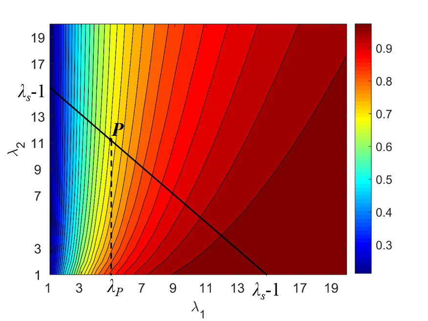
We consider the power allocation in Section III.D for L=2L=2. The first optimization problem is max⁡(R1∗+R2∗)\max\big(R^{*}_{1}+R^{*}_{2}\big), subject to λ1+λ2=λs\lambda_{1}+\lambda_{2}=\lambda_{s}. Figure 7 plots the maximum achievable sum rates and their optimal power allocation versus λs\lambda_{s}. It is seen that as λs\lambda_{s} increases, the optimal power allocation tends to become equal distribution, where the achievable sum rate enhances as ρ\rho grows from 0.10.1 to 0.50.5. The second optimization problem is to max⁡R1∗\max R^{*}_{1}, subjected to R2∗≥R2​i​n​fR^{*}_{2}\geq R_{2inf} and λ1+λ2=λs\lambda_{1}+\lambda_{2}=\lambda_{s}, as shown in Figure 8. Let PP denote the intersection of lines R=R2​i​n​fR=R_{2inf} and λ1+λ2=λs\lambda_{1}+\lambda_{2}=\lambda_{s}; and λP\lambda_{P} denote the xx-coordinates of PP. The feasible solution for the problem is that λ1=λs−λP,λ2=λP\lambda_{1}=\lambda_{s}-\lambda_{P},\lambda_{2}=\lambda_{P}.

Fig. 7: The optimal power allocation and achievable sum rate versus λs\lambda_{s}.
Refer to caption
Fig. 8: The achievable transmission rate of a single layer.

V-C Joint Detection and Decoding

Assume that λi=λa​v​e\lambda_{i}=\lambda_{ave} for 1≤i≤L1\leq i\leq L. The average symbol error rates for L=2L=2 and L=3L=3 of joint detection versus λa​v​e\lambda_{ave} are illustrated in Figures 9(a) and 9(b), respectively. Furthermore, we adopt a (12620,6310)(12620,6310) LDPC code for each signal layer, where the parity check matrix construction and low-complexity message pass decoding follow [36, 37] and [38]. The average bit error rates for L=2L=2 and L=3L=3 by joint detection and decoding versus λa​v​e\lambda_{ave} are shown in Figures 10(a) and 10(b), respectively. It is seen that for L=2L=2, ρ=0.5\rho=0.5 has the lowest error rate for both detection and decoding, which accords with the maximum achievable sum rate.

(a) The number of signal layer LL=2.
(b) The number of signal layer LL=3.
Fig. 9: The symbol error rate of joint detection.
(a) The number of signal layer LL=2.
(b) The number of signal layer LL=3.
Fig. 10: The bit error rate of joint detection and decoding with (12620,6310)(12620,6310) LDPC code.

VI Experimental Results for 22-layer-superimposed Transmission

We conduct offline experiments on the 22-layer-superposition transmission for optical wireless scattering communication to experimentally evaluate the proposed joint detection and decoding. At the transmitter side, a waveform generator is adopted to produce OOK signals. A Bias-Tee is employed to combine the AC and DC signals to drive the UV LED. At the receiver side, a photomultiplier tube (PMT) is employed as the photon-detector, which is integrated with an optical filter in a sealed box. The UV signal of wavelength around 280280nm can be detected, while the background radiation of other wavelengths is blocked. The PMT output signal is attenuated by an attenuator, amplified by an amplifier, and then filtered by a low-pass filter, which is then sampled by the oscilloscope. Finally, the photon counting processing, HMM-based MAP joint detection and decoding are realized in the received-side personal computer (PC) based on the sampled waveforms from the oscilloscope. Table I shows the specification of experimental equipment, and Figures 11 and 12 illustrate the entire experimental block diagram and the test bed realizations, respectively.

Refer to caption
Fig. 11: Diagram of the experimental superimposed communication system.
Refer to caption
Fig. 12: Demonstration of the transmitter-side (left) and receiver-side (right) test beds.
TABLE I: Specification of device for experiment.
UV LED Model TO-3zz PO#2036
Wavelength 280280nm
Optical filter Peak transmission 28.228.2%
Aperture size Φ​31.5\Phi 31.5mm ×28.3\times 28.3mm
PMT Model R7154
Spectral response 160160nm ∼\sim 320320nm
Dark counts <10<10 per second
Detection bandwidth >200>200MHz

In the experiment, the background radiation intensity is around 150150 photoelectrons per second in the indoor environment (λ0≈1.5×10⁻⁴)(\lambda_{0}\approx 1.5\times 10^{-4}). Furthermore, we adopt the following parameters for two signal layers: symbol duration Ts=1​μ​sT_{s}=1\mu s; ρ=0.5\rho=0.5; uniform power allocation for 22 signal layers (λ1=λ2=λa​v​e)(\lambda_{1}=\lambda_{2}=\lambda_{ave}); the same parity check matrix construction and decoding algorithm of LDPC codes as those in simulation; and the uniform prior probabilities for 0−10-1 symbols. For each λa​v​e\lambda_{ave}, we implement MAP joint detection and decoding and count the bit error rate based on the transmission of 10001000 frames (1.262×10⁷CLOSE(1.262\times 10^{7} random bits)).

We experimentally evaluate channel estimation for L=2,ρ1=0.5L=2,\rho_{1}=0.5, where we exploit a 255255-bit m sequence as a pilot sequence 𝒛p\boldsymbol{z}^{p}. For Lp=1L_{p}=1, 𝒛1p=𝒛p\boldsymbol{z}^{p}_{1}=\boldsymbol{z}^{p}; and for Lp=2L_{p}=2, 𝒛1p=𝒛2p=𝒛p\boldsymbol{z}^{p}_{1}=\boldsymbol{z}^{p}_{2}=\boldsymbol{z}^{p}. The performance of channel estimation versus the number of iterations is illustrated in Figure 14(a), where the result of Lp=2L_{p}=2 is from the ML estimation. It is implied that real time estimation for both Lp=0L_{p}=0 and 11 can converge to the ML solution; and assisted by the pilot sequence, the convergency of Lp=1L_{p}=1 is faster than Lp=0L_{p}=0. Furthermore, higher λ𝒔i\lambda_{\boldsymbol{s}_{i}} with large receiver-side SNR can lead to faster convergence, which is close to the simulation result on the channel estimation with the same system parameters, as shown in Figure 14(b).

Fig. 13: The average symbol and bit error rate of 22-layer superimposed communication from simulation and experimental measurements.
(a) Convergence of channel estimation from experiments.
(b) Convergence of channel estimation from simulations.
Fig. 14: Convergence of channel estimation from both experiments and simulations.

Moreover, the MAP detection with and without LDPC code (denoted as EXP) is evaluated in Figure 13, where the simulation results with the same channel parameters (denoted as SL) is plotted for comparison. It is seen that the experimental results on the channel estimation, symbol detection and joint detection/decoding are close to the simulation results, which illustrates the feasibility of the proposed channel estimation and signal detection approaches in real communication scenarios.

VII Conclusion

We have proposed superposition transmission for optical wireless scattering communication based on HMM. We have obtained the achievable rates of proposed superposition transmission, and proposed the EM-based channel estimation and joint detection and decoding. The performance of the proposed approaches are verified by numerical results. Moreover, for two- and three-layer transmission, both simulation and experimental results are employed to validate the feasibility of the proposed algorithms for channel estimation as well as joint detection and decoding.

VIII Appendix

VIII-A Comparison of Achievable Rates between OOK and 2-Pulse-Position Modulations (2-PPM)

The mutual information of single-use OOK modulation is given by

IO​O​K​(X,N)=max0<q<1⁡{ℋ⁡[∑Xq∈{0,1}ℙ⁡(Xq)​ℙO​O​K​(N|Xq)]−∑Xq∈{0,1}ℙ⁡(Xq)​ℋ​[ℙO​O​K​(N|Xq)]},\displaystyle\mathrm{I}_{OOK}(X;N)=\max\limits_{0<q<1}\Bigg\{\mathcal{H}\bigg[\sum_{X_{q}\in\{0,1\}}{\mathbb{P}(X_{q})\mathbb{P}_{OOK}(N|X_{q})}\bigg]-\sum_{X_{q}\in\{0,1\}}{\mathbb{P}(X_{q})\mathcal{H}\big[\mathbb{P}_{OOK}(N|X_{q})\big]}\Bigg\}, (36)

and that of 2-PPM is given by

I2−P​P​M(X;N1,N2)=max0<q<1max0<τ<1{ℋ[∑Xq∈{0,1}ℙ(Xq)ℙ2−P​P​M(N1,N2|Xq,τ)]−∑Xq∈{0,1}ℙ(Xq)ℋ[ℙ2−P​P​M(N1,N2|Xq,τ)]},\displaystyle\mathrm{I}_{2-PPM}(X;N_{1},N_{2})=\max\limits_{0<q<1}\max\limits_{0<\tau<1}\Bigg\{\mathcal{H}\bigg[\sum_{X_{q}\in\{0,1\}}{\mathbb{P}(X_{q})\mathbb{P}_{2-PPM}(N_{1},N_{2}|X_{q},\tau)\bigg]}-\sum_{X_{q}\in\{0,1\}}{\mathbb{P}(X_{q})\mathcal{H}\big[\mathbb{P}_{2-PPM}(N_{1},N_{2}|X_{q},\tau)\big]}\Bigg\}, (37)

where Xq∼{q,1−q}X_{q}\sim\{q,1-q\};

ℙO​O​K​(N|Xq=0)\displaystyle\mathbb{P}_{OOK}(N|X_{q}=0) =λ0NN!​e−λ0,\displaystyle=\frac{\lambda_{0}^{N}}{N!}e^{-\lambda_{0}}, (38)
ℙO​O​K​(N|Xq=1)\displaystyle\mathbb{P}_{OOK}(N|X_{q}=1) =(λ0+λ1)NN!​e−(λ0+λ1),\displaystyle=\frac{(\lambda_{0}+\lambda_{1})^{N}}{N!}e^{-(\lambda_{0}+\lambda_{1})},
ℙ2−P​P​M(N1,N2|Xq=0,τ)\displaystyle\mathbb{P}_{2-PPM}(N_{1},N_{2}|X_{q}=0,\tau) =τN1​λ0N1​(1−τ)N2​(λ0+λ1)N2N1!​N2!​e−τ​λ0−(1−τ)​(λ0+λ1),\displaystyle=\frac{\tau^{N_{1}}\lambda_{0}^{N_{1}}(1-\tau)^{N_{2}}(\lambda_{0}+\lambda_{1})^{N_{2}}}{N_{1}!N_{2}!}e^{-\tau\lambda_{0}-(1-\tau)(\lambda_{0}+\lambda_{1})},
ℙ2−P​P​M(N1,N2|Xq=1,τ)\displaystyle\mathbb{P}_{2-PPM}(N_{1},N_{2}|X_{q}=1,\tau) =τN1​(λ0+λ1)N1​(1−τ)N2​λ0N2N1!​N2!​e−τ⁡(λ0+λ1)−(1−τ)​λ0;\displaystyle=\frac{\tau^{N_{1}}(\lambda_{0}+\lambda_{1})^{N_{1}}(1-\tau)^{N_{2}}\lambda_{0}^{N_{2}}}{N_{1}!N_{2}!}e^{-\tau(\lambda_{0}+\lambda_{1})-(1-\tau)\lambda_{0}};

λ1\lambda_{1} denotes the mean number of detected photoelectrons in each symbol duration; N,N1,N2N,N_{1},N_{2} denote the number of received photoelectrons; and τ\tau denotes the duty ratio of the pulse in each symbol duration for 2-PPM. The achievable rates of OOK and 2-PPM modulation are compared in Figure 15, where OOK modulation shows higher achievable rate.

Fig. 15: The comparison between OOK and 2-PPM modulations with background intensity 1×1041\times 10^{4} per second.

VIII-B Proof of State Transition Matrix

For k=(t​ mod ​L)+1k=(t\text{ mod }L)+1, we have ⌈t+1−k+1L⌉=⌈t−k+1L⌉+1\lceil\frac{t+1-k+1}{L}\rceil=\lceil\frac{t-k+1}{L}\rceil+1, and ⌈t+1−r+1L⌉=⌈t−r+1L⌉\lceil\frac{t+1-r+1}{L}\rceil=\lceil\frac{t-r+1}{L}\rceil for r≠kr\neq k. Due to 𝑺t=[z1,⌈tL⌉,z2,⌈t−1L⌉,…,zL,⌈t−L+1L⌉]T\boldsymbol{S}_{t}=[z_{1,\lceil\frac{t}{L}\rceil},z_{2,\lceil\frac{t-1}{L}\rceil},\dots,z_{L,\lceil\frac{t-L+1}{L}\rceil}]^{T}, the rr-th element of 𝑺t\boldsymbol{S}_{t} and 𝑺t+1\boldsymbol{S}_{t+1} must satisfy zr,⌈t−r+1L⌉=zr,⌈t+1−r+1L⌉z_{r,\lceil\frac{t-r+1}{L}\rceil}=z_{r,\lceil\frac{t+1-r+1}{L}\rceil} for r≠kr\neq k. Consequently, The state transition probability ℙ⁡(𝑺t+1=𝒔t+1,j|𝑺t=𝒔t,i)=0\mathbb{P}(\boldsymbol{S}_{t+1}=\boldsymbol{s}_{t+1,j}|\boldsymbol{S}_{t}=\boldsymbol{s}_{t,i})=0, if zr,⌈t−r+1L⌉≠zr,⌈t+1−r+1L⌉z_{r,\lceil\frac{t-r+1}{L}\rceil}\neq z_{r,\lceil\frac{t+1-r+1}{L}\rceil}; and ℙ⁡(𝑺t+1=𝒔t+1,j|𝑺t=𝒔t,i)=ℙ⁡(zk,⌈t+1−k+1L⌉|zk,⌈t−k+1L⌉)\mathbb{P}(\boldsymbol{S}_{t+1}=\boldsymbol{s}_{t+1,j}|\boldsymbol{S}_{t}=\boldsymbol{s}_{t,i})=\mathbb{P}(z_{k,\lceil\frac{t+1-k+1}{L}\rceil}|z_{k,\lceil\frac{t-k+1}{L}\rceil}). Furthermore, zk,⌈t+1−k+1L⌉z_{k,\lceil\frac{t+1-k+1}{L}\rceil} is independent with zk,⌈t−k+1L⌉z_{k,\lceil\frac{t-k+1}{L}\rceil}, hence we have ℙ⁡(zk,⌈t+1−k+1L⌉|zk,⌈t−k+1L⌉)=qk,⌈t+1−k+1L⌉zk,⌈t+1−k+1L⌉​(1−qk,⌈t+1−k+1L⌉)zk,⌈t+1−k+1L⌉\mathbb{P}(z_{k,\lceil\frac{t+1-k+1}{L}\rceil}|z_{k,\lceil\frac{t-k+1}{L}\rceil})=q_{k,\lceil\frac{t+1-k+1}{L}\rceil}^{z_{k,\lceil\frac{t+1-k+1}{L}\rceil}}(1-q_{k,\lceil\frac{t+1-k+1}{L}\rceil})^{z_{k,\lceil\frac{t+1-k+1}{L}\rceil}}. In addition, zi,⌈t−i+1L⌉=𝑺t⋅𝒆iz_{i,\lceil\frac{t-i+1}{L}\rceil}=\boldsymbol{S}_{t}\cdot\boldsymbol{e}_{i} for 1≤i≤L1\leq i\leq L. Therefore, zr,⌈t−r+1L⌉≠zr,⌈t+1−r+1L⌉z_{r,\lceil\frac{t-r+1}{L}\rceil}\neq z_{r,\lceil\frac{t+1-r+1}{L}\rceil} is equivalent with (𝒔t+1,j⋅𝒆r)⊙(𝒔t,i⋅𝒆r)=0\big(\boldsymbol{s}_{t+1,j}\cdot\boldsymbol{e}_{r}\big)\odot\big(\boldsymbol{s}_{t,i}\cdot\boldsymbol{e}_{r}\big)=0, and ℙ⁡(𝑺t+1=𝒔t+1,j|𝑺t=𝒔t,i)\mathbb{P}(\boldsymbol{S}_{t+1}=\boldsymbol{s}_{t+1,j}|\boldsymbol{S}_{t}=\boldsymbol{s}_{t,i}) can be simplified into Equation (4).

VIII-C Proof of Chain Rules on Conditional Probabilities

We prove the proposition based on the following chain rule on the probability of received signal given two users since the numbers of received photoelectrons in different chips are independent of each other,

ℙ⁡(𝑵T|𝒁ℒ)\displaystyle\mathbb{P}(\boldsymbol{N}_{T}|\boldsymbol{Z}_{\mathcal{L}}) =∏t=1Tℙ⁡(Nt|Z1,⌈tL⌉,Z2,⌈t−1L⌉,…,ZL,⌈t−L+1L⌉).\displaystyle=\prod^{T}_{t=1}\mathbb{P}(N_{t}|Z_{1,\lceil\frac{t}{L}\rceil},Z_{2,\lceil\frac{t-1}{L}\rceil},\dots,Z_{L,\lceil\frac{t-L+1}{L}\rceil}). (39)

Consequently, Equation (12) can be proved by

ℙ⁡(𝒁k|𝒁ℒ\k,𝑵T)\displaystyle\mathbb{P}(\boldsymbol{Z}_{k}|\boldsymbol{Z}_{\mathcal{L}\backslash k},\boldsymbol{N}_{T}) =ℙ(Zk,1,𝒁k,[2,L]|{Zi,⌈t1−i+1L⌉},{Nt1},{Zi,⌈t~−i+1L⌉},{Nt~})\displaystyle=\mathbb{P}\big(Z_{k,1},\boldsymbol{Z}_{k,[2,L]}|\{Z_{i,\lceil\frac{{t_{1}}-i+1}{L}\rceil}\},\{N_{{t_{1}}}\},\{Z_{i,\lceil\frac{{\tilde{t}}-i+1}{L}\rceil}\},\{N_{{\tilde{t}}}\}\big) (40)
=ℙ(Zk,1,𝒁k,[2,L],{Nt1},{Nt~}∣{Zi,⌈t1−i+1L⌉},{Zi,⌈t~−i+1L⌉})∑Zk,1∑𝒁k,[2,L]ℙ(Zk,1,𝒁k,[2,L],{Nt1},{Nt~}∣{Zi,⌈t1−i+1L⌉},{Zi,⌈t~−i+1L⌉})\displaystyle=\frac{\mathbb{P}\big(Z_{k,1},\boldsymbol{Z}_{k,[2,L]},\{N_{{t_{1}}}\},\{N_{{\tilde{t}}}\}\mid\{Z_{i,\lceil\frac{{t_{1}}-i+1}{L}\rceil}\},\{Z_{i,\lceil\frac{{\tilde{t}}-i+1}{L}\rceil}\}\big)}{\sum_{Z_{k,1}}\sum_{\boldsymbol{Z}_{k,[2,L]}}\mathbb{P}\big(Z_{k,1},\boldsymbol{Z}_{k,[2,L]},\{N_{{t_{1}}}\},\{N_{{\tilde{t}}}\}\mid\{Z_{i,\lceil\frac{{t_{1}}-i+1}{L}\rceil}\},\{Z_{i,\lceil\frac{{\tilde{t}}-i+1}{L}\rceil}\}\big)}
=ℙ⁡({Nt1}∣Zk,1,{Zi,⌈t1−i+1L⌉})​ℙ​(Zk,1)​ℙ​({Nt~}∣𝒁k,[2,L],{Zi,⌈t~−i+1L⌉})​ℙ​(𝒁k,[2,L])∑Zk,1∑𝒁k,[2,L]ℙ⁡({Nt1}∣Zk,1,{Zi,⌈t1−i+1L⌉})​ℙ​(Zk,1)​ℙ​({Nt~}∣𝒁k,[2,L],{Zi,⌈t~−i+1L⌉})​ℙ​(𝒁k,[2,L])\displaystyle=\frac{\mathbb{P}\big(\{N_{{t_{1}}}\}\mid Z_{k,1},\{Z_{i,\lceil\frac{{t_{1}}-i+1}{L}\rceil}\}\big)\mathbb{P}\big(Z_{k,1}\big)\mathbb{P}\big(\{N_{{\tilde{t}}}\}\mid\boldsymbol{Z}_{k,[2,L]},\{Z_{i,\lceil\frac{{\tilde{t}}-i+1}{L}\rceil}\}\big)\mathbb{P}\big(\boldsymbol{Z}_{k,[2,L]}\big)}{\sum_{Z_{k,1}}\sum_{\boldsymbol{Z}_{k,[2,L]}}\mathbb{P}\big(\{N_{{t_{1}}}\}\mid Z_{k,1},\{Z_{i,\lceil\frac{{t_{1}}-i+1}{L}\rceil}\}\big)\mathbb{P}\big(Z_{k,1}\big)\mathbb{P}\big(\{N_{{\tilde{t}}}\}\mid\boldsymbol{Z}_{k,[2,L]},\{Z_{i,\lceil\frac{{\tilde{t}}-i+1}{L}\rceil}\}\big)\mathbb{P}\big(\boldsymbol{Z}_{k,[2,L]}\big)}
=ℙ⁡({Nt1}∣Zk,1,{Zi,⌈t1−i+1L⌉})​ℙ​(Zk,1)∑Zk,1ℙ⁡({Nt1}∣Zk,1,{Zi,⌈t1−i+1L⌉})​ℙ​(Zk,1)​ℙ⁡({Nt~}∣𝒁k,[2,L],{Zi,⌈t~−i+1L⌉})​ℙ​(𝒁k,[2,L])∑𝒁k,[2,L]ℙ⁡({Nt~}∣𝒁k,[2,L],{Zi,⌈t~−i+1L⌉})​ℙ​(𝒁k,[2,L])\displaystyle=\frac{\mathbb{P}\big(\{N_{{t_{1}}}\}\mid Z_{k,1},\{Z_{i,\lceil\frac{{t_{1}}-i+1}{L}\rceil}\}\big)\mathbb{P}\big(Z_{k,1}\big)}{\sum_{Z_{k,1}}\mathbb{P}\big(\{N_{{t_{1}}}\}\mid Z_{k,1},\{Z_{i,\lceil\frac{{t_{1}}-i+1}{L}\rceil}\}\big)\mathbb{P}\big(Z_{k,1}\big)}\frac{\mathbb{P}\big(\{N_{{\tilde{t}}}\}\mid\boldsymbol{Z}_{k,[2,L]},\{Z_{i,\lceil\frac{{\tilde{t}}-i+1}{L}\rceil}\}\big)\mathbb{P}\big(\boldsymbol{Z}_{k,[2,L]}\big)}{\sum_{\boldsymbol{Z}_{k,[2,L]}}\mathbb{P}\big(\{N_{{\tilde{t}}}\}\mid\boldsymbol{Z}_{k,[2,L]},\{Z_{i,\lceil\frac{{\tilde{t}}-i+1}{L}\rceil}\}\big)\mathbb{P}\big(\boldsymbol{Z}_{k,[2,L]}\big)}
=ℙ⁡(Zk,1∣{Nt1},{Zi,⌈t1−i+1L⌉})​ℙ​(𝒁k,[2,L]∣{Nt~},{Zi,⌈t~−i+1L⌉}),\displaystyle=\mathbb{P}\big(Z_{k,1}\mid\{N_{{t_{1}}}\},\{Z_{i,\lceil\frac{{t_{1}}-i+1}{L}\rceil}\}\big)\mathbb{P}\big(\boldsymbol{Z}_{k,[2,L]}\mid\{N_{{\tilde{t}}}\},\{Z_{i,\lceil\frac{{\tilde{t}}-i+1}{L}\rceil}\}\big),

where 𝒁k,[2,M]=[Zk,2,Zk,2,…,Zk,M]\boldsymbol{Z}_{k,[2,M]}=[Z_{k,2},Z_{k,2},\dots,Z_{k,M}], and the indexes involved in the brackets i∈ℒ\ki\in\mathcal{L}\backslash k, k≤t1≤k+L−1k\leq t_{1}\leq k+L-1 and k+L≤t~≤k+M​L−1k+L\leq\tilde{t}\leq k+ML-1. Re-factorizing Equation (40), we have

ℙ⁡(𝒁k|𝒁ℳ\k,𝑵T)\displaystyle\mathbb{P}(\boldsymbol{Z}_{k}|\boldsymbol{Z}_{\mathcal{M}\backslash k},\boldsymbol{N}_{T}) =ℙ⁡(Zk,1∣{Nt1},{Zi,⌈t1−i+1L⌉})​ℙ​(Zk,2∣{Nt2},{Zi,⌈t2−i+1L⌉})​ℙ​(𝒁k,[3,M]∣{Nt~},{Zi,⌈t~−i+1L⌉}),\displaystyle=\mathbb{P}\big(Z_{k,1}\mid\{N_{{t_{1}}}\},\{Z_{i,\lceil\frac{{t_{1}}-i+1}{L}\rceil}\}\big)\mathbb{P}\big(Z_{k,2}\mid\{N_{{t_{2}}}\},\{Z_{i,\lceil\frac{{t_{2}}-i+1}{L}\rceil}\}\big)\mathbb{P}\big(\boldsymbol{Z}_{k,[3,M]}\mid\{N_{\tilde{t}}\},\{Z_{i,\lceil\frac{\tilde{t}-i+1}{L}\rceil}\}\big), (41)

where the indexes involved in the brackets i∈ℒ\ki\in\mathcal{L}\backslash k, k+L≤t2≤k+2​L−1k+L\leq t_{2}\leq k+2L-1 and k+2​L≤t~≤k+M​L−1k+2L\leq\tilde{t}\leq k+ML-1. Re-factorize Equation (41) for M−2M-2 times, we have

ℙ⁡(𝒁k|𝒁ℒ\k,𝑵T)=∏j=1Mℙ⁡(Zk,j|{Zi,⌈tj−i+1L⌉},{Ntj}),\displaystyle\mathbb{P}(\boldsymbol{Z}_{k}|\boldsymbol{Z}_{\mathcal{L}\backslash k},\boldsymbol{N}_{T})=\prod^{M}_{j=1}\mathbb{P}\big(Z_{k,j}|\{Z_{i,\lceil\frac{t_{j}-i+1}{L}\rceil}\},\{N_{t_{j}}\}\big), (42)

where the indexes involved in the brackets i∈ℒ\ki\in\mathcal{L}\backslash k and k+(j−1)​L≤tj≤k+j​L−1k+(j-1)L\leq t_{j}\leq k+jL-1.

VIII-D Proof of conditional entropies

We prove the proposition by Equation (43) based on Proposition 1.

H⁡(𝒁k|𝒁ℒ\k,𝑵T)\displaystyle\mathrm{H}(\boldsymbol{Z}_{k}|\boldsymbol{Z}_{\mathcal{L}\backslash k},\boldsymbol{N}_{T}) =∑𝒁ℒ∈ℬM​L∑𝑵T∈ℕTℙ⁡(𝒁ℒ,𝑵T)​log2⁡ℙ⁡(𝒁k|𝒁ℒ\k,𝑵T)\displaystyle=\sum_{\!\!\!\!\!\!\!\!\!\!\boldsymbol{Z}_{\mathcal{L}}\in\mathscr{B}^{ML}}\sum_{\boldsymbol{N}_{T}\in\mathbb{N}^{T}}\!\!\!\mathbb{P}(\boldsymbol{Z}_{\mathcal{L}},\boldsymbol{N}_{T})\log_{2}\mathbb{P}(\boldsymbol{Z}_{k}|\boldsymbol{Z}_{\mathcal{L}\backslash k},\boldsymbol{N}_{T}) (43)
=∑𝒁ℒ∈ℬM​Lℙ⁡(𝒁ℒ)​∑𝑵T∈ℕTℙ⁡(𝑵T|𝒁ℒ)​log2⁡ℙ⁡(𝒁k|𝒁ℒ\k,𝑵T)\displaystyle=\sum_{\boldsymbol{Z}_{\mathcal{L}}\in\mathscr{B}^{ML}}\mathbb{P}(\boldsymbol{Z}_{\mathcal{L}})\!\!\sum_{\boldsymbol{N}_{T}\in\mathbb{N}^{T}}\!\!\!\mathbb{P}(\boldsymbol{N}_{T}|\boldsymbol{Z}_{\mathcal{L}})\log_{2}\mathbb{P}(\boldsymbol{Z}_{k}|\boldsymbol{Z}_{\mathcal{L}\backslash k},\boldsymbol{N}_{T})
=∑𝒁ℒ∈ℬM​Lℙ⁡(𝒁ℒ)​∑𝑵T∈ℕTℙ⁡(𝑵T|𝒁ℒ)​log⁡∏j=1M2⁡ℙ⁡(Zk,j|{Zi,⌈tj−i+1L⌉},{Ntj})\displaystyle=\sum_{\boldsymbol{Z}_{\mathcal{L}}\in\mathscr{B}^{ML}}\mathbb{P}(\boldsymbol{Z}_{\mathcal{L}})\!\!\sum_{\boldsymbol{N}_{T}\in\mathbb{N}^{T}}\!\!\!\mathbb{P}(\boldsymbol{N}_{T}|\boldsymbol{Z}_{\mathcal{L}})\log_{2}\prod^{M}_{j=1}\mathbb{P}\big(Z_{k,j}|\{Z_{i,\lceil\frac{t_{j}-i+1}{L}\rceil}\},\{N_{t_{j}}\}\big)
=∑𝒁ℒ∈ℬM​Lℙ⁡(𝒁ℒ)​∑𝑵T∈ℕTℙ⁡(𝑵T|𝒁ℒ)​log⁡∏j=1M2⁡ℙ⁡(Zk,j,{Ntj}|{Zi,⌈tj−i+1L⌉})ℙ⁡({Ntj}|{Zi,⌈tj−i+1L⌉})\displaystyle=\sum_{\boldsymbol{Z}_{\mathcal{L}}\in\mathscr{B}^{ML}}\mathbb{P}(\boldsymbol{Z}_{\mathcal{L}})\!\!\sum_{\boldsymbol{N}_{T}\in\mathbb{N}^{T}}\!\!\!\mathbb{P}(\boldsymbol{N}_{T}|\boldsymbol{Z}_{\mathcal{L}})\log_{2}\prod^{M}_{j=1}\frac{\mathbb{P}\big(Z_{k,j},\{N_{t_{j}}\}|\{Z_{i,\lceil\frac{t_{j}-i+1}{L}\rceil}\}\big)}{\mathbb{P}\big(\{N_{t_{j}}\}|\{Z_{i,\lceil\frac{t_{j}-i+1}{L}\rceil}\}\big)}
=∑Mj=1∑Zk,j∈ℬ(∑Zi,⌈(t−i+1)/L⌉∈ℬ)k+(j−1)​L≤t≤k+j​L−1i∈ℒ\kℙ(Zk,j)[∏i∈ℒ\kℙ({Zi,⌈tj−i+1L⌉})]∑{Ntj}∈ℕLℙ({Ntj}|Zk,j,{Zi,⌈tj−i+1L⌉})\displaystyle=\sum^{M}_{j=1}\sum_{Z_{k,j}\in\mathscr{B}}\Big(\!\!\!\sum_{Z_{i,\lceil(t-i+1)/L\rceil}\in\mathscr{B}}\!\!\!\!\!\!\Big)^{k+(j-1)L\leq t\leq k+jL-1\hfill\atop i\in\mathcal{L}\backslash k\hfill}\!\!\!\!\!\!\!\!\!\!\!\!\!\!\!\!\mathbb{P}(Z_{k,j})\Bigg[\prod_{i\in\mathcal{L}\backslash k}\mathbb{P}(\{Z_{i,\lceil\frac{t_{j}-i+1}{L}\rceil}\})\Bigg]\sum_{\{N_{t_{j}}\}\in\mathbb{N}^{L}}\!\!\!\mathbb{P}(\{N_{t_{j}}\}|Z_{k,j},\{Z_{i,\lceil\frac{t_{j}-i+1}{L}\rceil}\})
log2⁡ℙ⁡(Zk,j,{Ntj}|{Zi,⌈tj−i+1L⌉})ℙ⁡({Ntj}|{Zi,⌈tj−i+1L⌉})\displaystyle\log_{2}\frac{\mathbb{P}\big(Z_{k,j},\{N_{t_{j}}\}|\{Z_{i,\lceil\frac{t_{j}-i+1}{L}\rceil}\}\big)}{\mathbb{P}\big(\{N_{t_{j}}\}|\{Z_{i,\lceil\frac{t_{j}-i+1}{L}\rceil}\}\big)}
=∑Mj=1∑Zk,j∈ℬ(∑Zi,⌈(t−i+1)/L⌉∈ℬ)k+(j−1)​L≤t≤k+j​L−1i∈ℒ\kℙ(Zk,j)[∏i∈ℒ\k∏t=k+(j−1)​Lk+j​L−1ℙ(Zi,⌈t−i+1L⌉)]∑{Ntj}∈ℕL[∏t=k+(j−1)​Lk+j​L−1ℙ(Nt|Zk,j,{Zi,⌈t−i+1L⌉})]\displaystyle=\sum^{M}_{j=1}\sum_{Z_{k,j}\in\mathscr{B}}\Big(\!\!\!\sum_{Z_{i,\lceil(t-i+1)/L\rceil}\in\mathscr{B}}\!\!\!\!\!\!\Big)^{k+(j-1)L\leq t\leq k+jL-1\hfill\atop i\in\mathcal{L}\backslash k\hfill}\!\!\!\!\!\!\!\!\!\!\!\!\!\!\!\!\mathbb{P}(Z_{k,j})\Bigg[\prod_{i\in\mathcal{L}\backslash k}\prod_{t=k+(j-1)L}^{k+jL-1}\mathbb{P}(Z_{i,\lceil\frac{t-i+1}{L}\rceil})\Bigg]\sum_{\{N_{t_{j}}\}\in\mathbb{N}^{L}}\Bigg[\prod_{t=k+(j-1)L}^{k+jL-1}\mathbb{P}(N_{t}|Z_{k,j},\{Z_{i,\lceil\frac{t-i+1}{L}\rceil}\})\Bigg]
log2⁡ℙ⁡(Zk,j,{Ntj}|{Zi,⌈tj−i+1L⌉})ℙ⁡({Ntj}|{Zi,⌈tj−i+1L⌉})\displaystyle\log_{2}\frac{\mathbb{P}\big(Z_{k,j},\{N_{t_{j}}\}|\{Z_{i,\lceil\frac{t_{j}-i+1}{L}\rceil}\}\big)}{\mathbb{P}\big(\{N_{t_{j}}\}|\{Z_{i,\lceil\frac{t_{j}-i+1}{L}\rceil}\}\big)}
=∑Mj=1∑Zk,j∈ℬ(∑Zi,⌈(t−i+1)/L⌉∈ℬ)k+(j−1)​L≤t≤k+j​L−1i∈ℒ\kℙ(Zk,j)[∏i∈ℒ\k∏t=k+(j−1)​Lk+j​L−1ℙ(Zi,⌈t−i+1L⌉)]∑{Ntj}∈ℕL[∏t=k+(j−1)​Lk+j​L−1ℙ(Nt|Zk,j,{Zi,⌈t−i+1L⌉})]\displaystyle=\sum^{M}_{j=1}\sum_{Z_{k,j}\in\mathscr{B}}\Big(\!\!\!\sum_{Z_{i,\lceil(t-i+1)/L\rceil}\in\mathscr{B}}\!\!\!\!\!\!\Big)^{k+(j-1)L\leq t\leq k+jL-1\hfill\atop i\in\mathcal{L}\backslash k\hfill}\!\!\!\!\!\!\!\!\!\!\!\!\!\!\!\!\mathbb{P}(Z_{k,j})\Bigg[\prod_{i\in\mathcal{L}\backslash k}\prod_{t=k+(j-1)L}^{k+jL-1}\mathbb{P}(Z_{i,\lceil\frac{t-i+1}{L}\rceil})\Bigg]\sum_{\{N_{t_{j}}\}\in\mathbb{N}^{L}}\Bigg[\prod_{t=k+(j-1)L}^{k+jL-1}\mathbb{P}(N_{t}|Z_{k,j},\{Z_{i,\lceil\frac{t-i+1}{L}\rceil}\})\Bigg]
log2⁡ℙ⁡(Zk,j)​∏t=k+(j−1)​Lk+j​L−1ℙ⁡(Nt|Zk,j,{Zi,⌈t−i+1L⌉})∑Zk,j∈ℬℙ⁡(Zk,j)​∏t=k+(j−1)​Lk+j​L−1ℙ⁡(Nt|Zk,j,{Zi,⌈t−i+1L⌉})\displaystyle\log_{2}\frac{\mathbb{P}\big(Z_{k,j}\big)\prod_{t=k+(j-1)L}^{k+jL-1}\mathbb{P}(N_{t}|Z_{k,j},\{Z_{i,\lceil\frac{t-i+1}{L}\rceil}\})}{\sum_{Z_{k,j}\in\mathscr{B}}\mathbb{P}\big(Z_{k,j}\big)\prod_{t=k+(j-1)L}^{k+jL-1}\mathbb{P}(N_{t}|Z_{k,j},\{Z_{i,\lceil\frac{t-i+1}{L}\rceil}\})}

Typically, for single user transmission, the prior probability of the transmitted symbols remains constant, i. e, qi,j=qq_{i,j}=q for 1≤i≤L1\leq i\leq L and 1≤j≤M1\leq j\leq M. Consequently, each term in ∑j=1M[∙]\sum^{M}_{j=1}[\bullet] remain constant for 2≤j≤M−12\leq j\leq M-1. When j=1j=1 or j=Mj=M, ⌈t−i+1L⌉\lceil\frac{t-i+1}{L}\rceil may equal 00 or M+1M+1, we define Zi,0=Zi,M+1=0Z_{i,0}=Z_{i,M+1}=0 for 1≤i≤L1\leq i\leq L due to the finite number of transmitted symbols. Neglecting the effect of j=1j=1 and j=Mj=M, we have that ∑j=1M∑Zk,j∈ℬ[∙]=M​∑Zk,j0∈ℬ[∙]\sum^{M}_{j=1}\sum_{Z_{k,j}\in\mathscr{B}}[\bullet]=M\sum_{Z_{k,j_{0}}\in\mathscr{B}}[\bullet], where j0j_{0} can take any integer value in [2,M−1][2,M-1]; and

⌈t−i+1L⌉={j0,if 1≤i<k,k+(j0−1)​L≤t≤i+j0​L−1;j0+1,if 1≤i<k,i+j0​L≤t≤k+j0​L−1;j0−1,if k<i≤L,k+(j0−1)​L≤t≤i+(j0−1)​L−1;j0,if k<i≤L,i+(j0−1)​L≤t≤k+j0​L−1.\Big\lceil\frac{t-i+1}{L}\Big\rceil=\left\{\begin{array}[]{ll}j_{0},&\textrm{if $1\leq i<k,k+(j_{0}-1)L\leq t\leq i+j_{0}L-1$};\\ j_{0}+1,&\textrm{if $1\leq i<k,i+j_{0}L\leq t\leq k+j_{0}L-1$};\\ j_{0}-1,&\textrm{if $k<i\leq L,k+(j_{0}-1)L\leq t\leq i+(j_{0}-1)L-1$};\\ j_{0},&\textrm{if $k<i\leq L,i+(j_{0}-1)L\leq t\leq k+j_{0}L-1$}.\end{array}\right. (44)

Letting j0=2j_{0}=2, we have the following simplified form of Equation (43),

H⁡(𝒁k|𝒁ℒ\k,𝑵T)\displaystyle\mathrm{H}(\boldsymbol{Z}_{k}|\boldsymbol{Z}_{\mathcal{L}\backslash k},\boldsymbol{N}_{T}) =M∑Zk∈ℬ(∑Zi,2∈ℬ∑Zi,3∈ℬ)1≤i<k(∑Zi,1∈ℬ∑Zi,2∈ℬ)k<i≤Lℙ(Zk)[∏1≤i<kℙ(Zi,2)ℙ(Zi,3)∏k<i≤Lℙ(Zi,1)ℙ(Zi,2)]\displaystyle=M\sum_{Z_{k}\in\mathscr{B}}\bigg(\sum_{Z_{i,2}\in\mathscr{B}}\sum_{Z_{i,3}\in\mathscr{B}}\bigg)^{1\leq i<k}\bigg(\sum_{Z_{i,1}\in\mathscr{B}}\sum_{Z_{i,2}\in\mathscr{B}}\bigg)^{k<i\leq L}\mathbb{P}(Z_{k})\Bigg[\prod_{1\leq i<k}\mathbb{P}(Z_{i,2})\mathbb{P}(Z_{i,3})\prod_{k<i\leq L}\mathbb{P}(Z_{i,1})\mathbb{P}(Z_{i,2})\Bigg] (45)
∑{Nk+L,…,Nk+2​L−1}∈ℕL[∏t=k+Lk+2​L−1ℙ⁡(Nt|Zk,{Zi,⌈t−i+1L⌉})]​log2​ℙ⁡(Zk)​∏t=k+Lk+2​L−1ℙ⁡(Nt|Zk,{Zi,⌈t−i+1L⌉})∑Zk∈ℬℙ⁡(Zk)​∏t=k+Lk+2​L−1ℙ⁡(Nt|Zk,{Zi,⌈t−i+1L⌉}).\displaystyle\sum_{\{N_{k+L},\ldots,N_{k+2L-1}\}\in\mathbb{N}^{L}}\Bigg[\prod_{t=k+L}^{k+2L-1}\mathbb{P}(N_{t}|Z_{k},\{Z_{i,\lceil\frac{t-i+1}{L}\rceil}\})\Bigg]\log_{2}\frac{\mathbb{P}\big(Z_{k}\big)\prod_{t=k+L}^{k+2L-1}\mathbb{P}(N_{t}|Z_{k},\{Z_{i,\lceil\frac{t-i+1}{L}\rceil}\})}{\sum_{Z_{k}\in\mathscr{B}}\mathbb{P}\big(Z_{k}\big)\prod_{t=k+L}^{k+2L-1}\mathbb{P}(N_{t}|Z_{k},\{Z_{i,\lceil\frac{t-i+1}{L}\rceil}\})}.

VIII-E Derivation of 𝚲^(v)\hat{\boldsymbol{\Lambda}}^{(v)} in the M-Step of Channel Estimation

The likelihood function is given by

ℒ⁡(𝑵p|λ𝒔i=λ^𝒔i(v))\displaystyle\mathcal{L}(\boldsymbol{N}^{p}|\lambda_{\boldsymbol{s}_{i}}=\hat{\lambda}^{(v)}_{\boldsymbol{s}_{i}}) =∑Tpt=1log∑𝒔i∈ℬL∖Lpℙ(𝑵p,𝑺pt=𝒔i|λ𝒔i=λ^(v)𝒔i)\displaystyle=\sum^{T_{p}}_{t=1}\log\sum_{\boldsymbol{s}_{i}\in\mathscr{B}^{L\setminus L_{p}}}\mathbb{P}(\boldsymbol{N}^{p},\boldsymbol{S}^{p}_{t}=\boldsymbol{s}_{i}|\lambda_{\boldsymbol{s}_{i}}=\hat{\lambda}^{(v)}_{\boldsymbol{s}_{i}}) (46)
≥∑t=1Tp∑𝒔i∈ℬL∖LpQ(v)​(𝑺tp=𝒔i)​log⁡ℙ⁡(𝑵p,𝑺tp=𝒔i|λ𝒔i=λ^𝒔i(v))Q(v)​(𝑺tp=𝒔i).\displaystyle\geq\sum^{T_{p}}_{t=1}\sum_{\boldsymbol{s}_{i}\in\mathscr{B}^{L\setminus L_{p}}}Q^{(v)}(\boldsymbol{S}^{p}_{t}=\boldsymbol{s}_{i})\log\frac{\mathbb{P}(\boldsymbol{N}^{p},\boldsymbol{S}^{p}_{t}=\boldsymbol{s}_{i}|\lambda_{\boldsymbol{s}_{i}}=\hat{\lambda}^{(v)}_{\boldsymbol{s}_{i}})}{Q^{(v)}(\boldsymbol{S}^{p}_{t}=\boldsymbol{s}_{i})}.

Letting ℒ~(v)​(𝑵p|λ𝒔i=λ^𝒔i(v))\tilde{\mathcal{L}}^{(v)}(\boldsymbol{N}^{p}|\lambda_{\boldsymbol{s}_{i}}=\hat{\lambda}^{(v)}_{\boldsymbol{s}_{i}}) denote the last term of above inequality, we have that

ℒ~(v)​(𝑵p|λ𝒔i=λ^𝒔i(v))∼∑t=1Tp∑𝒔i∈ℬL∖LpQ(v)​(𝑺tp=𝒔i)​(Ntp​log⁡τt​λ^𝒔i(v)−log⁡Ntp!−τt​λ^𝒔i(v)).\displaystyle\tilde{\mathcal{L}}^{(v)}(\boldsymbol{N}^{p}|\lambda_{\boldsymbol{s}_{i}}=\hat{\lambda}^{(v)}_{\boldsymbol{s}_{i}})\sim\!\!\sum^{T_{p}}_{t=1}\!\!\sum_{\boldsymbol{s}_{i}\in\mathscr{B}^{L\setminus L_{p}}}\!\!Q^{(v)}(\boldsymbol{S}^{p}_{t}=\boldsymbol{s}_{i})\Big(N^{p}_{t}\log\tau_{t}\hat{\lambda}^{(v)}_{\boldsymbol{s}_{i}}\!-\!\log N^{p}_{t}!-\tau_{t}\hat{\lambda}^{(v)}_{\boldsymbol{s}_{i}}\Big).

Hence, the partial derivative of likelihood function is given by

∂∂λ𝒔i(v)​ℒ~(v)​(𝑵p=𝒏|λ𝒔i=λ^𝒔i(v))=∑t=1TpQ(v)​(𝑺tp=𝒔i)​(Ntpλ^𝒔i(v)−τt).\displaystyle\frac{\partial}{\partial\lambda^{(v)}_{\boldsymbol{s}_{i}}}\tilde{\mathcal{L}}^{(v)}(\boldsymbol{N}^{p}=\boldsymbol{n}|\lambda_{\boldsymbol{s}_{i}}=\hat{\lambda}^{(v)}_{\boldsymbol{s}_{i}})=\sum^{T_{p}}_{t=1}Q^{(v)}(\boldsymbol{S}^{p}_{t}=\boldsymbol{s}_{i})\Bigg(\frac{N^{p}_{t}}{\hat{\lambda}^{(v)}_{\boldsymbol{s}_{i}}}-\tau_{t}\Bigg). (47)

Letting ∂∂λ𝒔j​ℒ​(𝑵p=𝒏|λ𝒔j=λ^𝒔j(v))=0\frac{\partial}{\partial\lambda_{\boldsymbol{s}_{j}}}\mathcal{L}(\boldsymbol{N}^{p}=\boldsymbol{n}|\lambda_{\boldsymbol{s}_{j}}=\hat{\lambda}^{(v)}_{\boldsymbol{s}_{j}})=0, we have that

λ^𝒔j(v)\displaystyle\hat{\lambda}^{(v)}_{\boldsymbol{s}_{j}} =arg⁡max​ℒ~(v)​(𝑵p=𝒏|λ𝒔i=λ^𝒔i(v))=∑t=1TpQ(v)​(𝑺tp=𝒔i)​Ntp∑t=1TpQ(v)​(𝑺tp=𝒔i)​τt.\displaystyle=\arg\max\tilde{\mathcal{L}}^{(v)}(\boldsymbol{N}^{p}=\boldsymbol{n}|\lambda_{\boldsymbol{s}_{i}}=\hat{\lambda}^{(v)}_{\boldsymbol{s}_{i}})=\frac{\sum^{T_{p}}_{t=1}Q^{(v)}(\boldsymbol{S}^{p}_{t}=\boldsymbol{s}_{i})N^{p}_{t}}{\sum^{T_{p}}_{t=1}Q^{(v)}(\boldsymbol{S}^{p}_{t}=\boldsymbol{s}_{i})\tau_{t}}. (48)

References

  • [1] Z. Xu and B. M. Sadler, “Ultraviolet communications: potential and state-of-the-art,” IEEE Commun. Mag., vol. 46, no. 5, May 2008.
  • [2] C. Xu, H. Zhang, and J. Cheng, “Effects of haze particles and fog droplets on NLOS ultraviolet communication channels,” Opt. Express, vol. 23, no. 18, pp. 23259–23269, 2015.
  • [3] Y. Sun and Y. Zhan, “Closed-form impulse response model of non-line-of-sight single-scatter propagation,” JOSA A, vol. 33, no. 4, pp. 752–757, 2016.
  • [4] N. Raptis, E. Pikasis, and D. Syvridis, “Power losses in diffuse ultraviolet optical communications channels,” Opt. Lett., vol. 41, no. 18, pp. 4421–4424, 2016.
  • [5] K. Wang, C. Gong, D. Zou, and Z. Xu, “Turbulence channel modeling and non-parametric estimation for optical wireless scattering communication,” IEEE/OSA J. Lightwave Technol., vol. 35, pp. 2746–2756, Jul. 2017.
  • [6] M. Davis, “Capacity and cutoff rate for Poisson-type channels,” IEEE Trans. Inform. Theory, vol. 26, no. 6, pp. 710–715, Jun. 1980.
  • [7] A. D. Wyner, “Capacity and error exponent for the direct detection photon channel. I-II,” IEEE Trans. Inform. Theory, vol. 34, no. 6, pp. 1449–1461, Jun. 1988.
  • [8] M. R. Frey, “Information capacity of the Poisson channel,” IEEE Trans. Inform. Theory, vol. 37, no. 2, pp. 244–256, Feb. 1991.
  • [9] A. Lapidoth and S. M. Moser, “On the capacity of the discrete-time Poisson channel,” IEEE Trans. Inform. Theory, vol. 55, no. 1, pp. 303–322, Jan. 2009.
  • [10] A. Lapidoth, J. H. Shapiro, V. Venkatesan, and L. Wang, “The discrete-time Poisson channel at low input powers,” IEEE Trans. Inform. Theory, vol. 57, no. 6, pp. 3260–3272, Jun. 2011.
  • [11] K. Chakraborty and P. Narayan, “The Poisson fading channel,” IEEE Trans. Inform. Theory, vol. 53, pp. 2349–2364, Jul. 2007.
  • [12] K. Chakraborty, S. Dey, and M. Franceschetti, “Outage capacity of MIMO Poisson fading channels,” IEEE Trans. Inform. Theory, vol. 54, pp. 4887–4907, Nov. 2008.
  • [13] L. Lai, Y. Liang, and S. S. Shitz, “On the capacity bounds for Poisson interference channels,” IEEE Trans. Inform. Theory, vol. 61, pp. 223–238, Jan. 2015.
  • [14] H. Kim, B. Nachman, and A. El Gamal, “Superposition coding is almost always optimal for the Poisson broadcast channel,” IEEE Trans. Inform. Theory, vol. 62, pp. 1782–1794, Apr. 2016.
  • [15] N. Mehravari and T. Berger, “Poisson multiple-access contention with binary feedback,” IEEE Trans. Inform. Theory, vol. 30, no. 5, pp. 745–751, May 1984.
  • [16] A. Lapidoth and S. Shamai, “The Poisson multiple-access channel,” IEEE Trans. Inform. Theory, vol. 44, no. 2, pp. 488–501, Feb. 1998.
  • [17] S. I. Bross, M. V. Burnashev, and S. Shamai, “Error exponents for the two-user Poisson multiple-access channel,” IEEE Trans. Inform. Theory, vol. 47, no. 5, pp. 1999–2016, May 2001.
  • [18] G. Wang, C. Gong, and Z. Xu, “Signal characterization for multiple access non-line of sight scattering communication,” IEEE Trans. Commun., vol. 66, pp. 4138–4154, Sept. 2018.
  • [19] D. Raychaudhuri, “Performance analysis of random access packet-switched code division multiple access systems,” IEEE Trans. on Commun., vol. 29, no. 6, pp. 895–901, 1981.
  • [20] H. Ding, G. Chen, A. K. Majumdar, B. M. Sadler, and Z. Xu, “Correction to Modeling of non-line-of-sight ultraviolet scattering channels for communication,” IEEE J. Select. Areas Commun., vol. 29, pp. 250–250, Jan. 2011.
  • [21] Y. Zuo, H. Xiao, J. Wu, W. Li, and J. Lin, “Closed-form path loss model of non-line-of-sight ultraviolet single-scatter propagation,” Opt. Lett., vol. 38, pp. 2116–2118, Dec. 2013.
  • [22] C. Gong and Z. Xu, “Channel estimation and signal detection for optical wireless scattering communication with inter-symbol interference,” IEEE Trans. Wireless Commun., vol. 14, pp. 5326–5337, Oct. 2015.
  • [23] C. Gong and Z. Xu, “LMMSE SIMO receiver for short-range non-line-of-sight scattering communication,” IEEE Trans. Wireless Commun., vol. 14, pp. 5338–5349, Oct. 2015.
  • [24] C. Gong and Z. Xu, “Non-line of sight optical wireless relaying with the photon counting receiver: A count-and-forward protocol,” IEEE Trans. Wireless Commun., vol. 14, pp. 376–388, Jan. 2015.
  • [25] L. Rabiner and B. Juang, “An introduction to hidden Markov models,” IEEE ASSP Mag., vol. 3, no. 1, pp. 4–16, Jun. 1986.
  • [26] Y. Ephraim and N. Merhav, “Hidden markov processes,” IEEE Trans. Inform. Theory, vol. 48, no. 6, pp. 1518–1569, Jun. 2002.
  • [27] X. Liu, C. Gong, B. Liu, S. Li, and Z. Xu, “Hidden markov model based signal characterization for weak light communication,” IEEE/OSA J. Lightwave technol., vol. 36, pp. 1730–1738, Sept. 2018.
  • [28] T. K. Moon, “The expectation-maximization algorithm,” IEEE Signal Processing Mag., vol. 13, no. 6, pp. 47–60, Nov. 1996.
  • [29] A. P. Dempster, N. M. Laird, and D. B. Rubin, “Maximum likelihood from incomplete data via the EM algorithm,” Journal of the royal statistical society. Series B (methodological), pp. 1–38, 1977.
  • [30] G. D. Forney, “The viterbi algorithm,” Proc. IEEE, vol. 61, no. 3, pp. 268–278, Mar. 1973.
  • [31] L. Bahl, J. Cocke, F. Jelinek, and J. Raviv, “Optimal decoding of linear codes for minimizing symbol error rate (corresp.),” IEEE Trans. Inform. Theory, vol. 20, no. 2, pp. 284–287, Feb. 1974.
  • [32] J. Hagenauer, E. Offer, and L. Papke, “Iterative decoding of binary block and convolutional codes,” IEEE Trans. Inform. Theory, vol. 42, no. 2, pp. 429–445, Feb. 1996.
  • [33] S. Benedetto, D. Divsalar, G. Montorsi, and F. Pollara, “A soft-input soft-output APP module for iterative decoding of concatenated codes,” IEEE Commun. Lett., vol. 1, no. 1, pp. 22–24, Jan. 1997.
  • [34] T. M. Cover and J. A. Thomas, Elements of information theory. John Wiley & Sons, 2012.
  • [35] D. Hernando, V. Crespi, and G. Cybenko, “Efficient computation of the hidden Markov model entropy for a given observation sequence,” IEEE Trans. Inform. Theory, vol. 51, no. 7, pp. 2681–2685, Jul. 2005.
  • [36] M. Yang, W. E. Ryan, and Y. Li, “Design of efficiently encodable moderate-length high-rate irregular LDPC codes,” IEEE Trans. Commun., vol. 52, no. 4, pp. 564–571, Apr. 2004.
  • [37] M. P. Fossorier, “Quasicyclic low-density parity-check codes from circulant permutation matrices,” IEEE Trans. Inform. Theory, vol. 50, no. 8, pp. 1788–1793, Aug. 2004.
  • [38] J. Chen, A. Dholakia, E. Eleftheriou, M. P. Fossorier, and X.-Y. Hu, “Reduced-complexity decoding of LDPC codes,” IEEE Trans. Commun., vol. 53, no. 8, pp. 1288–1299, Aug. 2005.