Optimal Harvest-or-Transmit Strategy for Energy Harvesting Underlay Cognitive Radio Network

After some manipulations in the constraints, the equivalent convex MINLP $\textbf{P}_{2}$ of optimization problem $\textbf{P}_{1}$ is given as:

where $f(\bar{\mathbf{p}}_{s})=\sum_{i=1}^{M}\log_{2}\left(1+\frac{h_{ss}^{i}p_{s}^{i}}{\sigma^{2}+h_{ps}^{i}p_{p}^{i}}\right)+\sum_{i=M+1}^{N}\log_{2}\left(1+\frac{h_{ss}^{i}p_{s}^{i}}{\sigma^{2}}\right)$. The equivalence between (1) and (2) can be understood as follows. When $I_{H}^{i}=1$ for some $i\leq M$, the constraints (2c) or (2d) results in $p_{s}^{i}\leq 0$, which along with constraint $p_{s}^{i}\geq 0$ results in $p_{s}^{i}=0$. In this case, constraint (2e) would consider only those $p_{s}^{i}$’s which are positive. On the other hand when $I_{H}^{i}=1$ for some $i\leq M$, the constraint (2d) given an outer bound on $p_{s}^{i}$ and hence, has no effect. In this case, the constraints (2e) and (2f) will dominate and represent the energy causality constraints in (1e) and (1f).

The problem (2) is a convex MINLP problem since the objective function is concave in $\bar{\mathbf{p}}_{s}$ and the constraints contain affine inequalities. Since the continuous variable $\bar{\mathbf{p}}_{s}$ and the integer variable $\bar{\mathbf{I}}_{H}$ are now linearly separable, this problem can be solved efficiently using GBD algorithm [15].

In iteration $(l-1)$, we obtain an optimal $\bar{\mathbf{I}}_{H}^{(l-1)*}$ from $(l-1)^{th}$ iteration. Then, the primal problem in iteration $l$ is given as:

The optimization problem (4) is convex in $\bar{\mathbf{p}}_{s}$ [16] and can be solved using CVX [17]. The solution of the primal problem in $l$th iteration, $\bar{\mathbf{p}}^{(l)*}_{s}$ is used to obtain the solution of the master problem in next iterate, $\bar{\mathbf{I}}^{(l)*}_{H}$ for fixed $\bar{\mathbf{p}}_{s}$ and dual variables $\theta,\bar{\mathbf{\boldsymbol{\lambda}}},\bar{\mathbf{\boldsymbol{\gamma}}},\bar{\mathbf{\boldsymbol{\delta}}}$ and $\bar{\mathbf{\boldsymbol{\mu}}}$ associated with constraints (2c), (2d), (2e), (2f) and (2g) respectively.

The Lagrangian of the primal problem is given in (3). The Karush-Kuhn-Tucker (KKT) stationarity conditions are:

where $\Psi_{i}=\frac{h_{ss}^{i}}{\sigma^{2}+h_{ps}^{i}p_{p}^{i}+h_{ss}^{i}p_{s}^{i*}},\,\forall i$. The complementary slackness conditions are

where $\zeta=\left\{\sum_{j=1}^{M}p_{p}^{i}+E_{0}\right\}$. The dual variables associated with non-negativity constraints can be neglected for mathematical ease. However these constraints can be included later by projection onto the positive orthant. Using the KKT conditions, the optimal transmit power in $l$th iteration is given as:

where $\zeta_{1}=\theta^{*}+\mu_{1}^{*}h_{sp}^{1}+\sum_{j=1}^{M-1}\gamma^{*}_{j}+\sum_{j=1}^{N-M}\delta_{j}^{*}$, $\zeta_{i}=\mu_{i}^{*}h_{sp}^{i}+\lambda^{*}_{i-1}+\sum_{j=i-1}^{M-1}\gamma_{j}^{*}+\sum_{j=1}^{N-M}\delta_{j}^{*},\,i=2,\ldots,M$, and $[x]^{+}$ represents $\max\{x,0\}$. The optimal primal and dual variables in $l$th iterations are obtained using CVX [17]. The master problem for $l$th iteration is explained in next subsection.

We require the Lagrangian of the primal problem for the formulation of master problem, which is given in (3) on the top of the next page, where $\theta,\bar{\mathbf{\boldsymbol{\lambda}}},\bar{\mathbf{\boldsymbol{\gamma}}},\bar{\mathbf{\boldsymbol{\delta}}}$ and $\bar{\mathbf{\boldsymbol{\mu}}}$ are Lagrange multipliers for constraints (2c), (2d), (2e), (2f) and (2g) respectively. Let $\theta^{*},\bar{\mathbf{\boldsymbol{\lambda}}}^{*},\bar{\mathbf{\boldsymbol{\gamma}}}^{*},\bar{\mathbf{\boldsymbol{\delta}}}^{*}$ and $\bar{\mathbf{\boldsymbol{\mu}}}^{*}$ be the optimal Lagrangian variables. For given $\bar{\mathbf{p}}_{s}^{(l)*},\theta^{(l)*},\bar{\mathbf{\boldsymbol{\lambda}}}^{(l)*},\bar{\mathbf{\boldsymbol{\gamma}}}^{(l)*},\bar{\mathbf{\boldsymbol{\delta}}}^{(l)*}$ and $\bar{\mathbf{\boldsymbol{\mu}}}^{(l)*}$ obtained from primal problem in $l$th iteration, we formulate the master problem as:

The problem (8) is a mixed integer linear program (MILP) of $t$ and $\bar{\mathbf{I}}_{H}$ and hence, can be solved optimally using MOSEK [18].

GBD Algorithm: In the $l$th iteration, the master problem gives a solution $t$, an upper bound to the solution of original problem $\textbf{P}_{1}$. Also, in each iteration, one additional constraint (8b) is added to the master problem. Hence, the optimum of the master problem is non-increasing with number of iterations.

The primal problem gives a solution which is a lower bound to the optimum of original problem $\textbf{P}_{1}$ as it provides solution for fixed $\bar{\mathbf{I}}_{H}$. In each iteration, the lower bound is set equal to the maximum of the lower bounds obtained in current and previous iteration.

In the $l$th iteration the primal problem is solved for the solution obtained by master problem in $(l-1)$th iteration. Then, for the obtained solution of the primal problem in iteration $l$, we solve the master problem. This process continues and due to non-increasing (non-decreasing) nature of the upper bound (lower bound), optimal solution can be obtained the GBD algorithm converges in finite number of iterations [15].

The primal problem is convex and can be solved in polynomial time. However, the master problem is NP-hard as it is an integer programming problem. However, GBD can be solved efficiently using any commercial optimization software such as MOSEK [18]. The GBD algorithm is summarized in Algorithm 1, where $\mathcal{S}$ is a set of constraint (8b) in which an additional constraint is added in each iteration.

In Fig. 2, the effect of $P_{int}$ on the average EH and average Tx time for the first $M$ slots is shown. After $M$ slots, the PU becomes silent and the SU can not harvest RF energy from it. We assume that the PT transmits with power $p_{p}=1$ W in all the $M$ slots and initial energy in the battery $E_{0}=2$ J. It is evident that as $P_{int}$ decreases, the average EH time increases and average Tx time decreases (the average Tx time is the duration as long as PT remains active). When $P_{int}$ approaches zero, average EH-time approaches $M$ and average Tx-time approaches 0, i.e., the ST harvests energy as long as PT is active.

Fig. 3 shows the average achievable rate of ST under the optimal policy for different energy harvesting efficiency and different interference constraints at PR. The average is obtained over different channel realizations. For the simulation purpose, the number of primary slots, $M$ is assumed to be $N-2$. From the Fig. 3, it is evident that as the interference constraint at the primary receiver loosens, i.e., $P_{int}$ increases, and thus secondary transmitter is able to transmit with higher power, which results in higher achievable rate. When the interference constraint becomes too stringent, the secondary transmitter can not transmit as long as the PU is present. So, in this case, it harvests in first $M$ slots and transmits in remaining $N-M$ slots with total available energy of $E_{0}+M\alpha p_{p}$ and since ST does not get enough time to transmit, its achievable rate decreases as $P_{int}$ decreases.

Fig. 4 shows the comparison between the optimal and the myopic policy proposed in [12]. Since each slot at the ST is dedicated for either harvesting energy from the PU or transmitting its data, for smaller number of slots, the ST may not use the available slots efficiently for its transmission and therefore, the average achievable rate in our policy is less than that of in [12]. However, as the number of secondary slots $N$ increases, the proposed policy outperforms the myopic policy [12] as shown in Fig. 4. This is because in our policy, the ST takes the future channel gains into account and optimizes its transmit power over all the slots jointly.

Fig. 5 shows the average achievable rate versus the power transmitted by PT for fixed $\alpha$ and different values of $P_{int}$ averaged over different channel realizations. For simulation purpose we assumed $M$ and $N$ to be 6 and 10 respectively and $\alpha=0.9$. From the figure, it is inferred that the rate increases with $p_{p}$ because with increasing $p_{p}$, ST harvests more energy in each harvesting slot and can transmit with higher power.

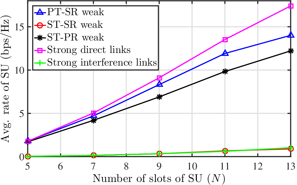
Fig. 6 shows the effect of different channel conditions on achievable rate. For simulation purpose, we assume the variance of weak links to be 0.01 and variance of strong links to be 0.1, $E_{0}=2$ J and $\alpha=0.9$. From the figure, it can be observed that when direct links are strong, the achievable rate is maximum as due to weak interference links, ST causes less interference to PR and receives less interference from PT. This allows ST to increase its transmission power which results in higher rate. The weak ST-SR and strong interference link case performs worst in all the scenarios because in both of these cases, SR receives more interference from PT and ST causes more interference to PR due to which ST can not transmit with higher power. Also, when ST-PR and PT-SR links are weak, performance degrades due to similar reasons.

References

- [1] X. Huang, T. Han, and N. Ansari, “On green-energy-powered cognitive radio networks,” IEEE Commun. Survey & Tutorials, vol. 17, pp. 827–842, Second 2015.
- [2] S. Park, H. Kim, and D. Hong, “Cognitive radio networks with energy harvesting,” IEEE Trans. Wireless Commun., vol. 12, pp. 1386–1397, Mar. 2013.
- [3] Pratibha, K. H. Li, and K. C. Teh, “Dynamic cooperative sensing-access policy for energy-harvesting cognitive radio systems,” IEEE Trans. Veh. Technol., vol. 65, pp. 10137–10141, Dec. 2016.
- [4] S. Park and D. Hong, “Optimal spectrum access for energy harvesting cognitive radio networks,” IEEE Trans. Wireless Commun., vol. 12, pp. 6166–6179, Dec. 2013.
- [5] W. Chung, S. Park, S. Lim, and D. Hong, “Optimal transmit power control for energy-harvesting cognitive radio system,” in Proc. 2013 IEEE VTC, pp. 1–5.
- [6] S. Yin, E. Zhang, Z. Qu, L. Yin, and S. Li, “Optimal cooperation strategy in cognitive radio systems with energy harvesting,” IEEE Trans. Wireless Commun., vol. 13, pp. 4693–4707, Sep. 2014.
- [7] C. Zhai, J. Liu, and L. Zheng, “Cooperative spectrum sharing with wireless energy harvesting in cognitive radio network,” IEEE Trans. Veh. Technol., vol. PP, no. 99, pp. 1–1, 2015.
- [8] G. Zheng, Z. Ho, E. A. Jorswieck, and B. Ottersten, “Information and energy cooperation in cognitive radio networks,” IEEE Trans. Signal Process., vol. 62, pp. 2290–2303, May 2014.
- [9] J. J. Pradha, S. S. Kalamkar, and A. Banerjee, “On information and energy cooperation in energy harvesting cognitive radio,” in Proc. 2015 IEEE PIMRC, pp. 943–948.
- [10] P. He and L. Zhao, “Optimal power control for energy harvesting cognitive radio networks,” in Proc. 2015 IEEE ICC, pp. 92–97.
- [11] K. Pathak and A. Banerjee, “On energy cooperation in energy harvesting underlay cognitive radio network,” in Proc. 2016 NCC, pp. 1–6.
- [12] V. Rakovic, D. Denkovski, Z. Hadzi-Velkov, and L. Gavrilovska, “Optimal time sharing in underlay cognitive radio systems with RF energy harvesting,” in Proc. 2015 IEEE ICC, pp. 7689–7694.
- [13] K. Pathak and A. Banerjee, “On optimal offline time sharing policy for energy harvesting underlay cognitive radio,” in Proc. 2016 SPCOM, pp. 1–5.
- [14] T. R. Ramya and S. Bhashyam, “On using channel prediction in adaptive beamforming systems,” in Proc. 2007 IEEE COMSWARE, pp. 1–6.
- [15] A. M. Geoffrion, “Generalized Benders decomposition,” Journal of Optimization Theory and Applications, vol. 10, no. 4, pp. 237–260.
- [16] S. Boyd and L. Vandenberghe, Convex Optimization. New York, NY, USA: Cambridge University Press, 2004.
- [17] M. Grant and S. Boyd, “CVX: Matlab software for disciplined convex programming, version 2.1.” http://cvxr.com/cvx, Mar. 2014.
- [18] “MOSEK Software.” http://www.mosek.com.