Local angles and dimension estimation
from data on manifolds

Suppose our data form an i.i.d. sample, $X_{1},\dots,X_{n}$ from a distribution $P$ on $\mathbb{R}^{m}$ with support on a Riemannian $C^{2}$ manifold $M$ of dimension $d<m$. Given a point $p\in M$, the question to be addressed is to determine the dimension $d$ of the tangent space of $M$ at $p$ using only information from sample points near $p$ (we want to allow for the value of $d$ to depend on the point $p$ and for $M$ to be disconnected).

The simplest version of our dimension identification procedure is described by the following steps:

1. (1)

   For an appropriate value of the constant $C$, to be specified below, let $k:=\lceil C\log(n)\rceil$. Assume, relabeling the sample if necessary, that $X_{1},\dots,X_{k}$ are the $k$ nearest neighbors of $p$ in the sample, according to the euclidean distance in $\mathbb{R}^{m}$.

2. (2)

   Define the angle-variance $U$-statistic, $U_{k,n}$, by the formula

   $$U_{k,n}:=\frac{1}{\binom{k}{2}}\sum_{1\leq i<j\leq k}\left(\arccos\left\langle\frac{X_{i}-p}{\|X_{i}-p\|},\frac{X_{j}-p}{\|X_{j}-p\|}\right\rangle-\frac{\pi}{2}\right)^{2},$$

   (2)

   where $\langle\cdot,\cdot\rangle$ denotes the dot product on $\mathbb{R}^{m}$.

3. (3)

   Estimate the unknown dimension $d$ as $\widehat{d}$, equal to the integer $r$ such that $\beta_{r}$ is closest to $U_{k,n}$, for a sufficiently large sample size $n$, where $\beta_{r}$ is the quantity defined by

   $$\beta_{r}:=\begin{cases}\frac{\pi^{2}}{4}-2\sum_{j=0}^{s}\frac{1}{(2j+1)^{2}}\text{ if $r-2=2s+1$ is odd or}\\ \frac{\pi^{2}}{12}-2\sum_{j=1}^{s}\frac{1}{(2j)^{2}}\text{ if $r-2=2s$ is even.}\par\end{cases}$$

   (3)

The key idea of our estimator goes as follows: For large $n$ and the chosen value of $k$, the nearest neighbors of $p$ in the data set, behave as uniform data on a small ball around $p$ in the embedded tangent space of $M$ at this point, and the corresponding unit vectors, $(X_{i}-p)/\|X_{i}-p\|$, are nearly uniform on the unit sphere of the tangent space, $S^{d-1}$. For uniform data on $S^{d-1}$, the expected angle between two random vectors is always $\pi/2$ (regardless of $d$), but the variance of this angle decreases rapidly with $d$. Formula (3) gives the value of this variance for every dimension $r$. Since our results below show that the $U$-statistic, $U_{k,n}$, will converge in probability to $\beta_{d}$ for the actual dimension of $M$ at $p$, estimation of $d$ by choosing the $r$ such that $\beta_{r}$ closest to $U_{k,n}$ will be consistent. An additional fact that helps in this convergence is that the variance of $U_{k,n}$, which depends on the fourth moment of the angles, is also converging rapidly to zero.

The following subsection establishes useful facts about angles between random points on the unit sphere $S^{d-1}$ of $\mathbb{R}^{d}$ and, in particular, about moments of the function

when computed on data uniformly distributed on $S^{d-1}$. Section 3, building on subsection 2.2, develops the theoretical results that serve as basis for the use of $U_{k,n}$ on manifolds.

At first glance the formulas for $\beta_{d}$ and $\sigma_{d}$ might seem a little complicated. In order to derive our results we need tangible decrease rates in terms of the dimension. The following claim gives us an easy way to interpret these quantities.

In this subsection we state the theoretical results that serve as basis for the proposed methodology. Proofs are given in the following subsection. The setting is the following: An i.i.d. sample, $X_{1},\dots,X_{n}$, is available from a distribution $P$ on $\mathbb{R}^{m}$. Additionally we have access to a distingushied point $p$, and near this point the data live on a Riemannian $C^{2}$ manifold $M$, of dimension $d<m$. Furthermore, at $p$ the distribution $P$ has a Lipschitz continuous non-vanishing density function $g$, with respect to the volume measure on $M$. Without loss of generality, we assume that $p=0$. Then, we have

In what follows, with a slight abuse of notation, we will write $X_{1},X_{2},\dots,X_{k}$ to denote the $k$ nearest neighbors of 0 in the sample and assume that these follow the distribution with density $g_{n}$ of Proposition 3.1. Let $\pi:\mathbb{R}^{m}\rightarrow T_{p}M$ be the orthogonal projection onto the (embedded) tangent space to $M$ at $p=0$. For a nonzero $X\in\mathbb{R}^{m}$, let $W:=\pi(X)$, $\widehat{X}:=\frac{X}{\|X\|}$ and $\widehat{W}:=\frac{W}{\|W\|}$. $\widehat{W}$ takes values in the $(d-1)$-dimensional unit sphere $S^{d-1}$ of the tangent space of $M$ at $0$.

Our first Lemma bounds the difference between the inner products $\langle\widehat{X_{i}},\widehat{X_{j}}\rangle$ and $\langle\widehat{W_{i}},\widehat{W_{j}}\rangle$ in terms of the length of projections. In this Lemma, the random nature of the $X_{i}$ is irrelevant.

Using Lemma 3.2, we can establish the following approximation. Let $X_{1},\dots,X_{k}$ be the $k$-nearest-neighbors from the sample to $p=0$ in $\mathbb{R}^{m}$ . Define $W_{i}$ and $\widehat{W_{i}}$ as above and let $V_{k,n}$ be given by the formula

When $X$ comes from the distribution producing the sample, but is restricted to fall very close to 0, the distribution of $\pi X$ will be nearly uniform in a ball centered at 0 in $T_{p}M$. This will allow us to establish a coupling between the normalized projection $\widehat{W}$ and a variable $Z$, uniformly distributed on the unit sphere of $T_{p}M$, an approximation that leads to the asymptotic distribution of $U_{k,n}$. Some geometric notation must be introduced to describe these results. Since near 0, $M\subseteq\mathbb{R}^{m}$ is a Riemannian submanifold of dimension $d$, it inherits, from the euclidean inner product in $\mathbb{R}^{m}$, a smoothly varying inner product $l_{p}:T_{p}M\times T_{p}M\rightarrow\mathbb{R}$, given by $l_{p}(u,v)=\langle i_{*}(u),i_{*}(v)\rangle$, where $i:M\rightarrow\mathbb{R}^{m}$ is the inclusion with differential $i_{*}$. This metric determines a differential $d$-form $\Omega_{M}$ which, in terms of local coordinates $\partial_{i}$ for $T_{p}M$ and dual coordinates $dx_{i}$ of $T_{p}M^{*}$ with $i=1,\dots d$, is given by $\Omega_{M}:=\sqrt{\det(\langle\partial_{i},\partial_{j}\rangle)_{1\leq i,j\leq d})}dx_{1}\wedge\dots\wedge dx_{d}$. The differential form endows $M$ with a volume measure $\nu(U)=\int_{U}\Omega_{M}$. We say that a random variable $A$ on $M$ has density $g:M\rightarrow\mathbb{R}$ if the distribution $\mu_{A}$ of $A$ satisfies $\mu_{A}(D)=\int_{D}g\Omega_{M}$ for all borel sets $D$ in $M$.

If $X$ is a random variable taking values on $M$ with density $g$ and $r$ is a positive real number, let $X(r)$ be a random variable with distribution $g_{r}$ given by the normalized restriction of $g$ to $M\cap B_{r}(0)$, that is:

Define $W(r):=\pi(X(r))$. The following geometric Lemma will be used for relating the densities of $X(r)$ and $W(r)$.

Let $D(r)$ be a random variable uniformly distributed in $B_{r}(0)\cap T_{p}M$ and note that $Z=\widehat{D}(r):=\frac{D(r)}{\|D(r)\|}$ is uniformly distributed on the unit sphere $S^{d-1}$, regardless of the value of $r$. Our next Lemma shows that under weak hypotheses there is a coupling between $W(r)$ and $D(r)$ which concentrates on the diagonal as $r$ decreases.

The previous Lemma leads to the asymptotic distribution of the statistic $U_{k,n}$.

This limit theorem is obtained by the various approximation steps given in the preliminary results together with the classical Central Limit Theorem for degenerate $U$ statistics, as described in Chapter 5 of [28]. Depending on the relative values of the $\lambda_{i}$’s appearing in the statement of the Theorem, it could happen that the limiting distribution just obtained approaches a Gaussian distribution as the dimension increases (this would happen if the $\lambda_{i}$ were such that Lindeberg’s condition holds).

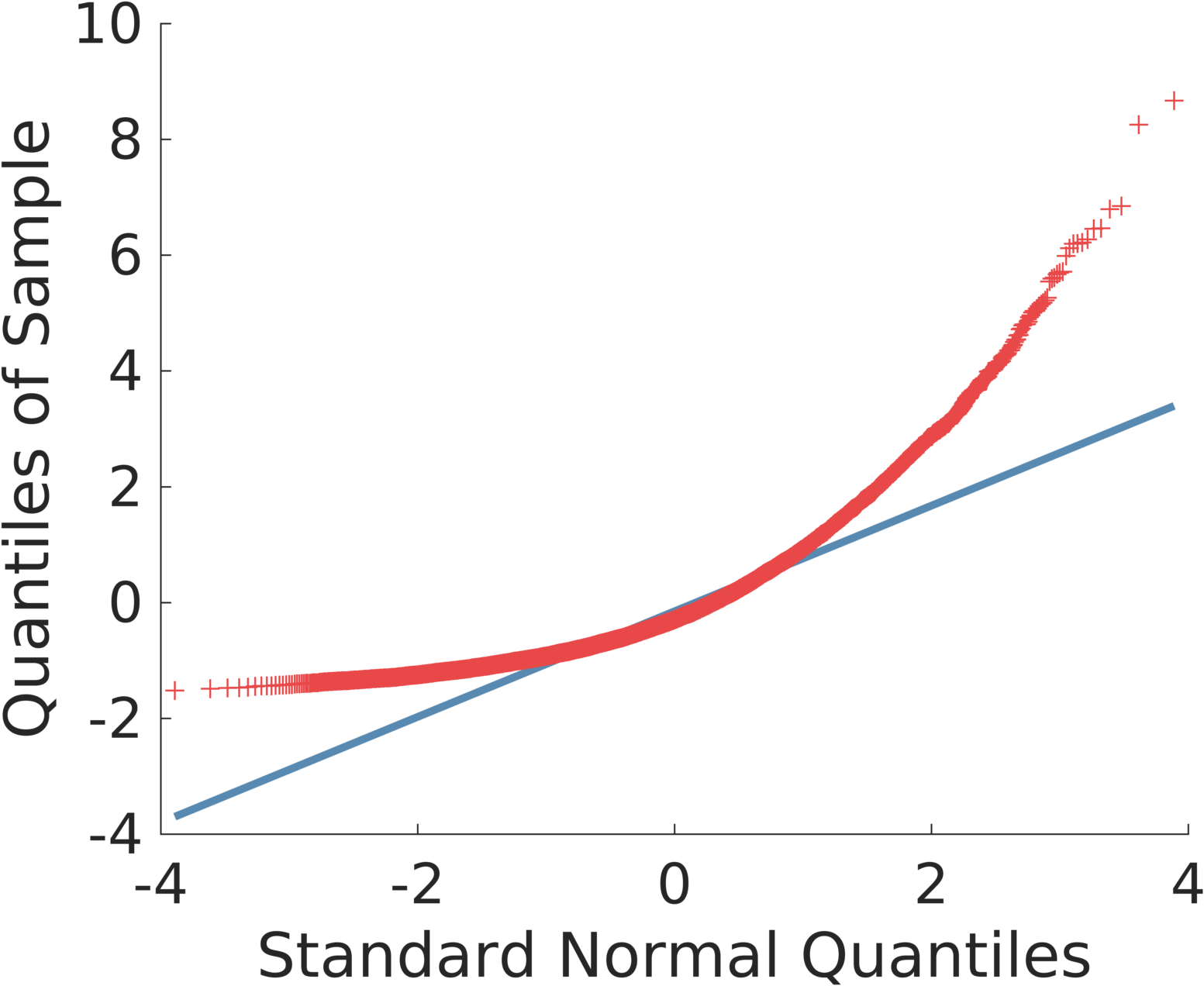
Although theoretical study of the $\lambda_{i}$’s is left for future work, we conjecture that as $d$ increases the limiting distribution converges to a Gaussian distribution. Numerical experiments seem to support our conjecture, see Figure 1.

In order to get a consistency result for our basic local dimension estimator, we will use the following fact.

Recall from Section 2 that our basic procedure estimates the dimension $d$ as $\widehat{d}$, equal to the integer $r$ such that $\beta_{r}$ is closest to $U_{k,n}$. This procedure is consistent, as stated next.

$\phantom{3}{}_{\phantom{3}}$

Proof of Proposition 3.1.
Let us recall a probability bound for the Binomial distribution. For $N$ an integer valued random variable with Binomial($n,p$) distribution and expected value $\lambda=np$, one of the Chernoff-Okamoto inequalities (see Section 1 in [16]) states that, for $t>0$, $\mathbb{P}(N\leq\lambda-t)\leq\exp(-t^{2}/2\lambda)$. Letting $t=\lambda/2$, we get

For fixed and small enough $r>0$, let $B_{r}(0)$ denote the ball of radius $r$ around $0\in\mathbb{R}^{m}$. For a random vector $X$, with the distribution $P$ of our sample $X_{1},X_{2},\dots,X_{n}$, by our assumptions on $P$ and $M$ near 0, we have that

where $\nu_{d}$ is the volume (Lebesgue measure) of the unit ball in $\mathbb{R}^{d}$ and $\alpha$ is a positive number. Let $N=N_{r}$ denote the amount of sample points that fall in $B_{r}(0)\cap M$. We have that $\lambda=\mathbb{E}(N)\leq\alpha\nu_{d}r^{d}n$. We choose $r$ such that $\lambda\leq C\ln n$, for a constant $C$ to be specified in a moment. Then, by (8), we get

Pick any value of $C>8$. For this choice, the bound in (9) will add to a finite value when summed over $n$. By the Borel-Cantelli Lemma, the inequality $N>\frac{C}{2}\ln n$ will hold for all $n$ sufficiently large. It follows that if $k=\frac{C}{2}\ln n$, the $k$-nearest-neighbors of 0 in the sample, will fall in $B_{r}(0)$ for every $n$ sufficiently large and the chosen value of $r$, namely

which is $\mbox{O}_{\Pr}((\ln n/n)^{1/d}))$. The proof of the first part of the Proposition ends by renaming $C$.
The statement of the second part of Proposition 3.1 is intuitive and has been used in the literature without proof. Luckily, Kaufmann and Reiss [18] provide a formal proof of these type of results in a very general setting. In particular, (ii) of Proposition 3.1 holds by formula (6) of [18]. $\Box$

Before proving Proposition 3.3, we need a Lemma on the behavior of the $\arccos$ function.

References

- [1] Aldous, D. and J. Shun (2010) Connected spatial networks over random points and a route-length statistic. Statistical Science 25, 275 - 288.
- [2] Arcones, M. A. and Giné, E. (1993) Limit Theory for -Processes. Annals of Probability 21, No. 3, 1494-1542.
- [3] Belkin, M. and Niyogi, P. (2004) Semi-supervised learning on Riemannian manifolds. Invited Paper inMachine Learning. Special Issue on Clustering 56, 209-239.
- [4] Bowman, A. W. and Foster, P. J. (1993) Adaptive smoothing and density-based tests of multivariate normality. Journal of the American Statistical Association 88 No. 422, 529-537.
- [5] Breiding, P., Kalisnik, S., Sturmfels, B. and Weinstein, M. (2018) Learning Algebraic Varieties from Samples. arXiv:1802.094[math.AG]
- [6] Brito, M. R., Quiroz, A. J. and Yukich, J. E. (2002) Graph theoretic procedures for dimension identification. Journal of Multivariate Analysis 81, 67-84.
- [7] Brito, M. R., Quiroz, A. J. and Yukich, (2013) Intrinsic dimension identification via graph-theoretic methods. Journal of Multivariate Analysis 116, 263–277.
- [8] Campadelli, P., Casiraghi, E., Ceruti, C. and Rozza, A. (2015) Intrinsic Dimension Estimation: Relevant Techniques and a Benchmark Framework. Mathematical Problems in Engineering 2015 Article ID: 759567, 21 pages.
- [9] Ceruti, C., Bassis, S., Rozza, A., Lombardi, G., Casiraghi, E. and Campadelli, P. (2014) DANCo: An intrinsic dimensionality estimator exploiting angle and norm concentration. Pattern Recognition 47, No. 8, 2569-2581.
- [10] Costa, J. A., Girotra, A. and Hero, A .O. (2005) Estimating local intrinsic dimension with k-nearest neighbor graphs. In IEEE/SP 13th Workshop on Statistical Signal Processing, 417-422. IEEE Conference Publication.
- [11] Devroye, Luc, Györfi, László and Lugosi, Gábor. (2013) A probabilistic theory of pattern recognition (Vol. 31). Springer Science and Business Media.
- [12] Duda, R. O., Hart, P. E. and Stork, D. G. (2001) Pattern Classification. 2nd. edition. John Wiley and Sons, New York.
- [13] Farahmand, A., Szepesvári, C. and Audibert, J-Y (2007) Manifold-adaptive dimension estimation. In Proceedings of the 24th International Conference on Machine Learning, Z. Ghahramani, editor, 265-272. ACM, New York.
- [14] Grassberger, P. and Procaccia, I. (1983) Measuring the strangeness of strange attractors. Physica 9D, 189-208.
- [15] Hein, M. and Audibert, J.-Y. (2005) Intrinsic dimensionality estimation of submanifolds in . In Proceedings of the 22nd International Conference on Machine learning, 289-296, ACM.
- [16] Janson, S. (2002). On concentration of probability. In Bollobás, B. (Ed.) Contemporary Combinatorics, 10. Proceedings of the Workshop on Probabilistic Combinatorics at the Paul Erdös Summer Research Center, Budapest, 1998, pp. 289-301.
- [17] Johnson, M. E. (1987) Multivariate Statistical Simulation. John Wiley and Sons, New York.
- [18] Kaufmann, E. and Reiss, R.-D. (1992) On Conditional Distribution of Nearest Neighbors. Journal of Multivariate Analysis 42, 67-76.
- [19] Kegl, B. (2003) Intrinsic dimension estimation using packing numbers. In Advances in Neural Information Processing Systems, Volume 15, Eds. S. Becker, S. Thrun and K. Obermayer. M.I.T. Press, Cambridge, Massachusetts.
- [20] Levina, E. and Bickel, P. J. (2005) Maximum likelihood estimation of intrinsic dimension. In Advances in Neural Information Processing Systems, Volume 17, Eds. L. K. Saul, Y. Weiss and L. Bottou.
- [21] Lombardi et. al., 2011 Lombardi, G., Rozza, A., Ceruti, C., Casiraghi, E. and Campadelli, P. (2011). Minimum Neighbor Distance Estimators of Intrinsic Dimension. In D. Gunopulos et al. (Eds.): ECML PKDD 2011, Part II, LNAI 6912, pp. 374-389. Springer-Verlag. Berlin.
- [22] Mardia, K. V., Kent, J. T. and Bibby, J. M. (1979) Multivariate Analysis. Academic Press, New York.
- [23] Penrose, M. D. and Yukich, J. E. (2001) Central limit theorems for some graphs in computational geometry. Annals of Applied Probability 11, 1005-1041.
- [24] Penrose, M. D. and Yukich, J. E. (2013) Limit theory for point processes in manifolds. Annals of Applied Probability 23, No. 6, 2161-2211.
- [25] Pettis, K. W., Bailey, T. A. Jain, A. K. and Dubes, R. C. (1979) An intrinsic dimensionality estimator from near-neighbor information. IEEE Transactions on Pattern Analysis and Machine Intelligence 1, 25-37.
- [26] Randles, R. H. and Wolfe, D. A. (1979) Introduction to the Theory of Nonparametric Statistics. John Wiley and Sons, New York.
- [27] Roweis, S. T. and Saul, L. K. (2000) Nonlinear dimensionality reduction by locally linear embedding. Science, 290, 2323-2326.
- [28] Serfling, R. J. (1980) Approximation Theorems of Mathematical Statistics. John Wiley and Sons, New York.
- [29] Sindhwani, V., Belkin, M. and Nigoyi, P. (2006) The Geometric Basis of Semi-supervised Learning. Book chapter in Semi-supervised Learning, O. Chapelle, B. Schölkopf and A. Zien, editors, M.I.T. Press, Cambridge, Massachusetts.
- [30] Södergren, A. (2011) On the distribution of angles between the N shortest vectors in a random lattice Journal of the London Mathematical Society, 84, No. 3, 749-764.
- [31] Sricharan, K. Raich, R. and Hero, A. O. (2010) Optimized intrinsic dimension estimation using nearest neighbor graphs. In IEEE International Conference on Acoustics, Speech and Signal Processing (ICASSP), 5418-5421. IEEE Conference Publication.
- [32] Steele, J. M., Shepp, L. A. and Eddy, W. F. (1987) On the number of leaves of a Euclidean minimal spanning tree. Journal of Applied Probability, 24, 809-826.
- [33] Tenenbaum, J. B., de Silva, V. and Langford, J. C. (2000) A global geometric framework for nonlinear dimensionality reduction. Science 290, 2319-2323.
- [34] Villani, C. (2009) Optimal Transport. Old and New. Volume 338 in series Grundlehren der matematischen Wissenschaften. Springer. Berlin, Heidelberg.
- [35] Yukich, J. E. (1998) Probability Theory of Classical Euclidean Optimization Problems. Lecture Notes in Mathematics, 1675, Springer, New York.