Multiple outbreaks in epidemic spreading with local vaccination and limited vaccines
Abstract
How to prevent the spread of human diseases is a great challenge for the scientific community and so far there are many studies in which immunization strategies have been developed. However, these kind of strategies usually do not consider that medical institutes may have limited vaccine resources available. In this manuscript, we explore the Susceptible-Infected-Recovered (SIR) model with local dynamic vaccination, and considering limited vaccines. In this model, susceptibles in contact with an infected individual, are vaccinated -with probability - and then get infected -with probability . However, when the fraction of immunized individuals reaches a threshold , the vaccination stops, after which only the infection is possible. In the steady state, besides the critical points and that separate a non-epidemic from an epidemic phase, we find for a range of another transition points, and , which correspond to a novel discontinuous phase transition. This critical value separates a phase where the amount of vaccines is sufficient, from a phase where the disease is strong enough to exhaust all the vaccination units. For a disease with fixed , the vaccination probability can be controlled in order to drastically reduce the number of infected individuals, using efficiently the available vaccines.
Furthermore, the temporal evolution of the system close to or , shows that after a peak of infection the system enters into a quasi-stationary state, with only a few infected cases. But if there are no more vaccines, these few infected individuals could originate a second outbreak, represented by a second peak of infection. This state of apparent calm, could be dangerous since it may lead to misleading conclusions and to an abandon of the strategies to control the disease.
I Introduction
Human interactions have a structure that can be well described in the form of a complex network [1, 2, 3, 4]. In the last few years, new technologies allowed us to record large amount of data of contact patterns [5, 6, 7, 8]. This data has become accessible to researches that use data-driven network modeling approaches to analyze and understand spreading in social systems, for example, how epidemic and even rumors spread in real populations.
Scientists have focused [9, 10, 11, 12, 13], on modeling and analyzing disease spreading since it can lead to catastrophic health consequences as well as large economic losses. Several mathematical approaches have been developed and used to study different epidemic models, improving the understanding of disease spreading on complex networks [14, 15] (and references therein).
Since one of the goals of health authorities is to minimize health catastrophes and economic impact of health policies, many studies have focused on establishing immunization and mitigation strategies for enhancing the functionality of a society and reduce the economic cost [16, 17]. For example, vaccination programs [18] are very efficient in providing immunity to individuals and as a consequence, the final number of infected people decreases considerably. However, these strategies are usually very expensive and unrealistic, because vaccines against new strains are usually not available during the initial propagation stage. As a consequence, non-pharmaceutical interventions are needed to protect the society. One of the most effective and studied strategy to slow an epidemic is quarantine. However, it has the disadvantage that full isolation has a negative impact on the economy of the region and it is difficult to implement it in a large population. Thus, it is important to find a balance between these two strategies. Another policy, such as social distancing strategies, have been modeled and implemented in order to reduce the average contact time between individuals [19, 20]. This kind of strategies, usually include closing schools, cough etiquette, travel restrictions, intermittent connections, etc. Unfortunately, in most cases, these strategies do not prevent a pandemic, but only delays its spread.
One of the most remarkable cases of a disease spreading was the pandemic occurred by the H1N1 strain in 2009, which caused about deaths. Initially, the disease propagated over the network of close contacts, and then through the airline network, transporting infected individuals to different cities, thus spreading the disease all over the world. One of the most used models to mimic these kind of epidemics is the Susceptible-Infected-Recovered () model [21, 22, 23, 24]. In this model an individual can be in only one of three possible states: Susceptible (S), Infected (I) or Recovered (R). An individual in state S in contact with an I, changes to an I state with probability . After a period of time the infected individual changes to an state and stops transmitting the disease. This model presents, in the steady state, two regimes governed by an effective probability of contagion , such that for the system is in an epidemic-free phase and for it is in an epidemic phase, where the disease reaches a high fraction of the population. The model has been also successfully applied to model the case of SARS and other diseases of influenza type [25, 26]. For decades, researchers have studied different scenarios of the epidemic model [27, 28, 29, 30] and develop mitigation strategies to prevent the epidemic [31, 32, 33, 34, 18], such as isolation, quarantine and random and targeted vaccination. Particularly, Valdez et al. [35] studied, using the SIR model, the effect of an intermittent social distancing strategy on the propagation of epidemics in adaptive complex networks. Based on local information, a susceptible individual interrupts the contact with an infected individual with a certain probability and restores it after a fixed period of time. In a similar way, Ref. [36] extended the model and was able to successfully predict the date of extinction of the Ebola’s outbreak in Liberia in . Ebola outbreaks have been studied by the scientific community due to the high impact of this epidemic on certain regions of southwest Africa, mainly in Guinea, Sierra Leona and Liberia. Fortunately, there exists available data for the scientific community enabling to study more accurately the behavior and propagation of this disease [36, 37].
During this Ebola outbreak, a vaccine trial has been performed and used in Guinea in 2015 in the capital city. It has been found that the strategy of the vaccine trial applied to mitigate the transmission of Ebola-Virus-Disease () in Guinea in 2015, was very efficient [38]. The vaccine trial tested the efficacy of an experimental vaccine against Ebola. The trial used a “ring” vaccination’ strategy based on the approach that was used to eradicate the smallpox [39]. This involves the identification of a newly diagnosed Ebola case, and then the vaccination of all his contacts and the contacts of those contacts, which are usually their family members, neighbors, co-workers and friends. In practical terms, the close contacts of a newly identified Ebola case have been vaccinated, if they consent to it. This is the basis of the motivation of the present study where we immunize the neighbors of an infected individual in network models. Moreover, the amount of vaccines, sometime due to economic restrictions, may not be enough to protect all the susceptible neighbors of the infected individuals during the whole spreading process. Thus, we propose and study here models with the scenario of limited vaccines availability, i.e. not enough for all the vulnerable population. Generally speaking, the available resources to control, avoid, or maybe enhance a spreading process are limited, and many studies have focused in how to optimally use these scarce resources against a disease [40], or even to deal with illicit drug usage [41].
We are interested in testing how this limited amount of accessible vaccines affects the spread of the epidemic. Motivated by this, we present here a model of localized vaccination that mimics the vaccine trial in Guinea, in which only neighbors of infected individuals could be immunized using limited vaccination units. This could help to understand how the propagation of a disease is affected by the localized and limited vaccination. Therefore, the question we wish to answer is how to use, in an efficiently way, this limited amount of vaccines with the aim of reducing the propagation of an epidemic.
In our model, the state of an individual can be Susceptible (S), Vaccinated (V), Infected (I) or Recovered (R). A susceptible individual in contact with an infected one will become vaccinated with probability , until the total number of vaccines is used. If he does not become vaccinated, then with probability he will become infected. Then, after a certain period of time , the infected individuals will recover.
Using an edge-based compartmental model and the generating functions theory [24, 42], we obtain and study the evolution equations for the fraction of S, I, R and V individuals and find a perfect agreement between theoretical and simulation results. Then, we study the steady state of the epidemic process, for which there is no more infected individuals. We find two different phases, an epidemic and a non-epidemic phase, separated by a critical threshold , which depend on . Below the disease can not spread and the fraction of recovered individuals approaches to zero. On the other hand if is fixed, there is a critical vaccination probability , above which the epidemic can not develop, since the disease is successfully blocked by immunized individuals.
Above , depending on the parameters, we find either a continuous phase transition or a discontinuous phase transition for a second epidemic break at higher critical threshold , which depends on . Similarly for fixed , below we find a discontinuous transition for in the fraction of recovered individuals. In Refs. [43, 44, 45] the authors also found a discontinuous transition but in the density of infected individuals, and using an endemic epidemic model (susceptible-infected-susceptible), where the recovery of sick individuals depends on the availability of healing resources.
We also find, that depending on the parameters there are values of and that characterize a crossover between two regimes, one for which the available amount of vaccines is sufficient to immunize the population during the whole process and the other in which it is not.
II The Model
At the initial state, all the individuals in the network are susceptible except one, the patient zero, which is in the infected compartment or state. Before spreading the disease, all the susceptible neighbors of this individual receive a vaccine with probability . Notice that this vaccination is local and dynamic, and is done through the links that connect infected to susceptible nodes. Then the patient zero will try to infect all its neighbors that have not been vaccinated, and this event will occur with probability . In the next time step of the process, all the susceptible neighbors of the infected nodes will be vaccinated with probability again or will be infected with probability . The infected individuals will move to the recovered state R after units of time since they become infected, and the vaccinated or immunized individuals will remain in state V. While the disease spreads through the population, the number of vaccinated people increases, until the health institutes run out of vaccines. We define as the fraction of available vaccines over the entire population. When this limit is reached, no more individuals can be immunized and hence those in the infected state will infect their neighbors with probability . In the steady state the epidemic is over when the fraction of infected individuals is zero, thus the individuals can only be in state S, R or V. For demonstration of the model see Fig. 1.
This model is clearly different from random vaccination, in which a fraction of individuals selected at random are immunized. In the random strategy, some vaccinated individuals may never be in contact with an infected individual and thus would not be vaccinated, in the present strategy. On the other hand the dynamical vaccination intends to create a barrier of immunized individuals that could stop the spreading of the disease, thus making a more effective usage of the available vaccines.

III Theoretical Formalism
The edge-based compartmental model (EBCM) [24, 8], was applied to model the SIR and was adapted by Valdez et al. for discrete time, and a fixed recovery time [27]. We can solve theoretically the evolution and the steady state of this model with unlimited vaccines [46] and also adapt it here for the limited case. The EBCM is based on a generating function formalism, implemented in branching and percolation processes on complex networks. This approach allows to study not only the steady state but also the temporal evolution of the process. First, we derive the general equations for the case of unlimited vaccines and then we explain the effect of the depletion of the vaccines. Denoting the fraction of susceptible, infected, vaccinated and recovered individuals at time by , , and , respectively, the EBCM approach lies on describing the evolution of the probability that a randomly chosen node is susceptible. In order to compute , a link is randomly chosen and then a direction is given, in which the node in the target of the arrow is called the root node, and the base is its neighbor, called base node. We denote to the probability that at time , the base node does not transmit the disease to the root node and neither induces the immunization of the root node. In this approach, the state of the base node can not be affected by the root node, so that we can treat the state of the root’s neighbors as independent [23, 24, 27]. A node remains as susceptible if none of its neighbors cause its infection or immunization, then the fraction of individuals in the susceptible state at time is given by
| (1) |
where is the generating function of the degree distribution, , of the network [47]. To compute we have to take into account all the possible states of the base node. Suppose an edge that connects the root node and the base node. Then, this edge has not been used yet to infect or vaccinate the root node if the base node is
- •
in state S, with probability .
- •
infected but did not spread the disease to the root node, nor induced the immunization of the root node, which is expressed by .
- •
in state R but during the time it was infected, it did not propagate the disease to the root node, nor induced vaccination to the root node. This probability is denoted by .
- •
vaccinated or immunized, with probability .
We summarize these probabilities in Table 1.
| Quantity | Possible states of the base node |
|---|---|
| Susceptible | |
| Infected and did not infect nor did it induce the vaccination of the root node | |
| Recovered and did not infect nor did it induce the vaccination of the root node | |
| Vaccinated |
In Fig. 2 a) we demonstrate the configurations of the root and the base node.

Thus, accounting all these cases (see Fig. 2 b), is given by
| (2) |
Similar to in Eq. (1), we can write an expression for (see Fig. 2 b). The neighbor of the root node, with degree , is in state S if the disease does not spread through its links and if none of its neighbors, omitting the root node, do not induce its vaccination. Recall that the edge coming from the root node is not considered. Hence the probability that the base node is susceptible at time is and thus,
| (3) |
where is the generating function of the excess degree distribution of the network and is the average degree [48]. The evolution equations that describe the process for unlimited vaccination, i.e. , are (see Appendix A for detailed derivation),
| (4) | ||||
In the first equation, decreases if the base node is infected at time , and induces the vaccination of the root node with probability , or if it spreads the disease to the root, with probability . Note that takes into account that the base node and the root node had no prior interaction. The second equation represents the evolution of the probability that the base node is in state S, which is the finite difference of (see Eq. (3)). The third equation is a bit more complicated. The root node has, with probability , an infected neighbor at time that did not induce its immunization or caused its infection. This probability changes if the infected base node causes the immunization of the root node or infects it, which is reflected in the first term. In the second term we have the susceptible individuals that become infected at time and will be in state I in the next time step. Unlike [27], where the authors used the EBCM to solve the classical SIR model, this term does not account all the variation of , since a fraction of the susceptible individuals go to state V. The fraction of the nodes in state S that go to state I is weighted with the factor , which is the probability that the disease spreads through a link. The last term in the 3rd equation takes into account the susceptible individuals that got infected at time units earlier, and did not change the state of the root node during this time. The probability that they do not spread the disease or induce the vaccination to the root node during this period of time is , where
| (5) |
and is the probability that during the period an infected base node did not infect nor induced the vaccination to the root node. Finally, the last equation takes into account the immunized neighbors of the root node. The variation of increases with time and is proportional to the negative change of . In this case the factor , is the probability that the link between the root node and the base node is used to immunize. We explain these additional probabilities in Table 2.
After computing using Eqs.(4), we can compute the evolution of the fraction of susceptible, infected and vaccinated individuals at time by,
| (6) | ||||
| Probability | Definition |
|---|---|
| The base node did not infect nor did it induce the vaccination of the root node | |
| A susceptible node adopts the state I if its state change | |
| A susceptible node adopts the state V if its state change | |
| A link is used to infect or vaccinate during units |
Notice than using these magnitudes we can compute the fraction of recovered individuals, . The derivation of these equations is similar to Eqs. (4). In the first equation, the change in the fraction of susceptible individuals is the finite difference of (Eq.(1)). Next, in the second equation the variation of the vaccinated individuals is proportional to the change in the susceptible individuals. This is since , and the factor takes into account the transition from state S to V. In the third equation, the change in the fraction of infected individuals is also proportional to the variation of the susceptible individuals, but here the factor is related to the transition from state S to I. Hence, is the fraction of new infected individuals at time . On the other hand, is the fraction of individuals that got infected temporal units earlier. Thus, this fraction represents the individuals that move to state R at time , and hence contribute negatively to the fraction of infected individuals.
The set of equations (4) and (6) describes the temporal evolution of the process with unlimited vaccines (). Now we assume that we have a limited amount of vaccination units, lower than the number of individuals in the system. Thus we impose a limit as the maximal fraction of vaccinated individuals.
The evolution of the system is the same as the unlimited case until reaches the vaccination limit, . At this point there is no available vaccines and thus the vaccination probability becomes zero, allowing the disease to spread without barriers. Hence the equations should be iterated normally until , and then setting for the rest of the process. Nevertheless, since in Eq. (6), changes by finite increments, it is unlikely that matches with exactly. Thus it is not clear when iterating the equations, the precise moment at which the immunization process has to be stopped. We explain in Appendix B the procedure that has been performed to solve this problem and to reproduce exactly the results from the computational simulations.
IV Results


We perform stochastic simulations of the localized and limited vaccination SIR model over single networks with nodes, whose degree distribution is Erdős Rényi (ER) with an average degree . The networks are built using the Molloy-Reed algorithm [49].
IV.1 Temporal Evolution
To demonstrate the validity of the theoretical formalism, in Fig. 3 we show simulations and theory of the temporal evolution of the process for an infection probability , a vaccination probability , a vaccination limit , and a recovery time . The dashed lines are the theoretical results from the EBCM described in the previous section, while the solid lines represent different realizations of the stochastic simulations. We can see the excellent agreement between the theoretical equations (6) and the simulation results.
It can be seen from Fig. 3 that initially, as the fraction of infected and vaccinated individuals increase with time, the fraction of susceptible individuals decreases. Each infected node reaches the state R after units of time and consequently the fraction of recovered individuals increases with time. In the classical SIR model, the fraction of infected individuals reaches a maximum and then decreases, but in our case of limited vaccines, after a specific time the behavior of the curves changes. At this time the system runs out of vaccine units and thus no more individuals can be immunized against the disease. At this point the fraction of susceptible nodes shows a plateau, since as seen in Fig. 3(b), the epidemic almost vanished. and there are only few infected individuals that can infect the susceptible people. This plateau, which is also observed for the recovered individuals (Fig. 3(c)), seems to indicate that the system begins to stabilize, since the magnitudes change slowly with time. However, when suddenly the vaccines are exhausted, the fraction of infected individuals starts to increase again, reaching a second peak (Fig. 3(b)) that could be even higher than the first one. This increase obviously cause a further decrease and increase of the susceptible and recovered individuals respectively. Finally the disease starts to fade away as the fraction of infected individuals decreases, then the system reaches the steady state and all the magnitudes stabilize.
From now on, in the rest of the manuscript, our results will be based only from the theoretical equations, since we find excellent agreement (Fig. 3) with the stochastic simulations.
Next we will show the temporal behavior of the process for different values of the infection probability, . In the standard SIR model, without vaccination, there is a critical value below which there is no epidemic. This value satisfies the equality [50], where is the transmissibility, the effective probability of contagion, and is the branching factor of the degree distribution of the network. and are the first and second moments of the degree distribution respectively. From this relation, in which , the critical infection probability can be obtained as [21]. In the present model of limited dynamical vaccination, the relation between and holds but in this case the transmissibility depends also on the vaccination probability (see Appendix D for the expression of ). Closed expressions of for are quite complicated, however for the critical infection probability is simply . We see that this probability depends on but not on the vaccination limit . Besides , in our model there are also specific values of associated with dramatic changes in the behavior of the magnitudes at the steady state. Unlike , these values depend on the number of immunization units. Next we will show how the magnitudes evolve with time when is one of these specific values.
Fig. 4 exhibits the temporal evolution of all magnitudes for , , and for several values of . For this particular set of parameters , nevertheless in this figure we will focus on another important value greater than , which we call . In Fig. 4 (a) , and


we observe that in this case the fraction of infected individuals shows only one peak, and also the other magnitudes show a standard behavior. However if the infection probability is just a little higher, , suddenly two peaks appear in the fraction of infected nodes, as seen in the inset of Fig. 4 (b). Similar to Fig. 3, when the fraction of vaccinated individuals reaches the vaccination limit, in this case , the fraction of susceptible and recovered nodes enter in a quasi-stationary state, in which they barely change. At this stage there is a negligible number of infected individuals, however since the vaccination stops, there are enough infected-susceptible pairs to start a second outbreak. This causes the second peak and a further decrease in the number of susceptible individuals, as well as a further increase in the fraction of recovered nodes. Thus, at the steady state experiences an abrupt transition with . We will see later in Figs. 5 and 7 how the nature of the abrupt transitions depends highly on the limited vaccines units, .
In Figs. 4 (c) and (d), for larger values of we observe that the two peaks start to get closer, until eventually they start to fuse together forming a single peak as in Fig. 4 (a), but much higher. On the other hand, for larger values the curves become smoother since there is only a single outbreak.
IV.2 Steady State
To understand how the results are affected by the infection probability , in Fig. 5 we show the fraction of vaccinated, recovered and susceptible individuals in the steady state as a function of for a fixed vaccination probability , and for different values of limited vaccines , for an ER network with . The green solid lines represent the case of unlimited vaccines, .i.e., . In Fig. 5 (a) we see that for increasing , the fraction of vaccinated individuals increases, since more infected individuals means more susceptible neighbors to immunize. Nevertheless, we observe that this curve reaches a maximum and then decreases for larger values of . This can be understood as follows. When the probability of infection becomes high, the majority of neighbors of an infected node get infected instead of being immunized, and thus there is a decrease in the fraction of vaccinated individuals [46]. It is important to point out that the existence of this maximum is highly influenced by the vaccination probability and the topology of the network. In Appendix E (Fig. 10) we show the fraction of vaccinated and recovered individuals at the steady state for networks with a heterogeneous power law degree distribution, and for different values of .
Next we observe what happens if we impose a limit on the fraction of available vaccines. For , represented by the red squares, we see in Fig. 5 (a) a plateau between two values of . This happens since V can not surpass the vaccination limit. The lower of these values is , which we introduce in Fig. 3, and we call the other , which is greater than (see Fig. 5 (a)). Between these two values is the range of for which V reaches its limit value, . Now we ask what is the effect of the vaccination limit on the fraction of recovered individuals. In Fig. 5 (b) we observe that between and , denoted by the vertical dashed lines, the curves of recovered fraction show significantly increased values compared to the case of unlimited vaccines. In this region at some value, , the vaccine units are exhausted, and then the disease spreads without barriers, affecting a great number of individuals that could not be immunized.
For example, for , represented in Fig. 5 by black triangles, we observe a similar behavior. In in this case , but an interesting phenomena takes place at where a discontinuous jump occurs due to the shortage of vaccination units. This abrupt transition, in Fig. 5 (b) and (c), can be understood from Figs. 4 (a) and (b). Below there is a single outbreak, while above it a second outbreak causes the abrupt jumps observed in Fig. 5. It is expected therefore that for , an even smaller supply of immunization units, the condition of the population becomes worse, as seen in Fig. 5. The curve with blue circles shows that there is no , and thus for any the fraction of infected is significantly higher, compared to the case of unlimited vaccines. The dashed lines that denote these points indicate the emergence of a second peak of infection, as can be seen in Figs. 4 (b) and (c).
In Fig. 5 (c) we show the fraction of susceptible individuals, which decrease with and also show a discontinuous jump at , associated with .


In Fig. 5 (d) we compute the time it takes the process to reach the steady state, as seen in Fig. 4. Processes near the transition point, usually have longer duration times compared to those far from this point, as found for example in the process of cascading failures [51, 52]. Taking this into consideration, we can see that for , represented in this figure by a green dotted line, there is only one peak at [46], which is associated with a continuous phase transition. This peak is seen for all , since the critical point does not depend on . However, for , and , represented respectively by a blue solid line, a dash-dotted black line, and a red dashed line, we observe another peak at longer times, which is located at , which depends on . Consequently, if we return to Fig. 4, where we show the temporal evolution for , we see indeed that for (Fig. 4 (b)) the process takes much longer time to reach the steady state compared to (Fig. 4 (a)).
Thus, we can infer that similar to , the probability of infection denotes a transition point, that separates a region in which the immunization strategy stops the spreading of the disease, and another in which the vaccination units are insufficient to stop it. On the other hand, we do not observe a peak at , indicating that this is not a transition point. Instead, this point denotes a crossover between the regime of insufficient vaccines and a regime in which the immunization units can not be used completely, since the probability of infection is too high. Moreover we recall that the existence of is related to the topology of the network, see Appendix E (Fig. 10). To see also how the curves of Fig. 5 behave for a different recovery time , see Fig. 9 in appendix E where we show the steady state for and for , the vaccination limit used in Fig. 3.
Next we fix the infection probability and analyze how the magnitudes at the steady state change with the vaccination probability . In Fig. 6 we show the fraction of recovered and vaccinated individuals as a function of for different vaccination limits. First we focus on the cases in Figs. 6 (a) and (c), and in Figs. 6 (b) and (d). Similar to Fig. 5 the fraction of vaccinated individuals increases with and reaches a maximum, after which it starts decreasing. This occurs because many of the paths that would be used by the disease to spread, are blocked by immunized individuals. Thus, since there are few people infected there are fewer contacts around them to vaccinate. Furthermore, there is a critical vaccination probability for which the disease stops to propagate, since all the paths are completely blocked due to vaccination. For we can show that [46]. We see that for these values of the amount of vaccines is sufficient. Next we examine smaller values of , for which the system runs out of vaccines at some point.
In all figures we observe that as increases from zero, the number of vaccinated individuals rises and the number of recovered individuals decreases, until a specific vaccination probability , for which the vaccines are depleted. We see in Fig. 6 (a) and Fig. 6 (b) that after this point the fraction of recovered individuals has a lower decline rate, being practically insignificant for small values of . For instance, from Fig. 6 (b) it is clear that vaccination with probability or yield the same results. However, suddenly at , a small increase in the fraction of immunized individuals can block many spreading paths of the disease, which results in a dramatic drop in the number of recovered individuals. This discontinuous jump is analogous to the behavior observed in Fig. 5 at , and one can easily relate to .
Thus, for a disease with fixed and for a fixed number of available vaccines , based on the vaccination rate we can predict the number of infected individuals in the system when the epidemic comes to an end. Furthermore and very importantly, for a given and , we can chose the optimal rate of vaccination, , such that the fraction of infected be minimal or even zero.


The numerical values of , , and can be calculated theoretically using the generating functions formalism and branching theory [53, 47] (see Appendix D for the derivation of the formula).
Finally in Fig. 7 we show the model phase diagrams, which exhibit different regions depending on the parameters. In Fig. 7 (a), where , the solid curve in the plane represents the values of for each , while the dashed curve represents . This curves enclose the vaccines-depletion region (in purple), where we see that for a small vaccination limit and a high infection probability the system runs out of immunization units. On the other hand, the region of sufficient vaccines (in yellow), is characterized by (i) low infection probabilities, for which little vaccines are needed to stop the disease, and (ii) if and are both high, the vaccines do not get exhausted. The reason for (ii) is that the disease rapidly spreads before all the vaccines can be used. Finally the dotted line represents the value of , below which there is no epidemic.
In Fig. 7 (b) we fix and show the phase diagram in the plane . Here the solid and dashed curves represent and respectively. Here we see that when increases the depletion region becomes broader because more vaccines are applied. However when further increases, the immunization strategy gets more effective against the disease, and then a smaller amount of vaccines is required to control the epidemic. Furthermore when , the disease can not propagate since all the paths are blocked by immunized individuals.


Using these phase diagrams we can learn how the regions of insufficient vaccines change with the available immunization resources in medical institutes, the infection probability, which depends on the disease, and the vaccination probability, which may depend on the medical workers.
V Discussion
In this manuscript we have explored the implications of a limited number of vaccines in the model with local vaccination. We find that at the steady state, there is a region of values of the infection probability , in which the medical institutions run out of immunization units. This region is delimited by and or, by and depending on the vaccination limit . We also find that is a transition point, at which the curve of recovered individuals has a discontinuous jump, whose height depends on . This type of behavior, in which a discontinuous transition is observed, has been seen when the dynamics of propagation of epidemics is coupled with social processes [54, 55]. Furthermore, we analyze the temporal evolution of the process close to . We find that for , the temporal evolution of the fraction of infected individuals presents two peaks. When the disease is about to vanish the vaccines are exhausted, and then the infection probability is sufficiently large for an extremely small fraction of infected individuals to cause a sudden second outbreak. On the contrary, we observed that is not a transition point but a crossover, and that its existence depends on the topology of the network.
On the other hand we analyze the steady state of the process as a function of , finding other points of interest. One of them is , below which the vaccination probability is too low to use all the vaccines, thus the immunization units are not exhausted but the epidemic is not effectively halted. Another point is , above which the vaccination probability is high enough to control the epidemic with the available immunization resources, and shows a discontinuous transition in the fraction of recovered individuals. These results are of significant importance since the vaccination probability is one of the few parameters that can be controlled by the health institutes. Thus, can be chosen to minimize the number of infected individuals or even halt the epidemic in the primary stages, according to the available resources.
We solved the model using an EBCM, finding an excellent agreement with the stochastic simulations. Also, we used the branching theory to find the values of , , and . In future studies we will analyze different features of the local vaccination model, as the immunization of first and second neighbors of infected individuals. Thus, intending imitate more accurately the ring vaccination strategy used against the Ebola outbreak in Guinea during .
Acknowledgements
SH thanks the Israel Science Foundation, ONR, the Israel Ministry of Science and Technology (MOST) with the Italy Ministry of Foreign Affairs, BSF-NSF, MOST with the Japan Science and Technology Agency, the BIU Center for Research in Applied Cryptography and Cyber Security, and DTRA (Grant no. HDTRA-1-10-1- 0014) for financial support. LAB wish to thank DTRA (Grant no. HDTRA-1-10-1- 0014) for financial support. MAD, LGAZ and LAB wish to thank to UNMdP and CONICET (PIP 00443/2014) for financial support.
Appendix A Edge-based compartmental model (EBCM)
In this appendix we derive the set of equations (4) using the EBCM. For simplicity we will assume continuous time and rates and of infection and vaccination respectively. Also the recovery time is replaced by a recovery rate . Once we derive the equations of temporal evolution we can adapt them for discrete time steps.
As we saw earlier the probability that the root node of the network, selected at random, do not get infected or vaccinated through a link by the base node is , and satisfies Eq. (2). This variable can change only if the link between the root and the base node is used to infect or vaccinate. Since these events occur with rates and respectively, thus
| (7) |
Therefore, since then
| (8) |
On the other hand, a node is in state if is not susceptible and if was more likely to receive a vaccine rather than be infected, hence
| (9) | ||||
Similar to Eq.(8) we can write
| (10) |
Next we study the variation of , the probability that the base node is recovered and also, that during the time it was infected did not cause the infection or the vaccination of the root node. Since individuals recover with rate hence
| (11) |
To obtain first we have to rewrite Eq.(7). The probability that the disease or the vaccination spread through at least one link to the root node is and thus
| (12) |
| (13) |
Now integrating this equation and considering that and are negligible at the beginning of the process, then simply
| (14) |
| (15) |
and finally using Eq.(7) we can write a single differential equation for
| (16) |
This equation together with , , and describes the evolution of the fraction of susceptible, infected, vaccinated and recovered individuals on a complex network for continuous time.
Alternatively, we can derive Eq. (2) with respect to time and use Eqs. (8), (10) and (11) to write a differential equation for
| (17) |
Appendix B Temporal evolution of the discrete-time equations close to the threshold
When iterating Eqs. (4), one approach is to set in the temporal step that would surpass , ensuring that , but not that at the steady state. This would cause many fluctuations when computing as a function of at the steady state. Thus, to reproduce exactly the results from the computational simulations another approach should be used. Next we detail the procedure we use to avoid this fluctuations. At time we calculate , and if it turns out that is greater than , then we calculate what is the value of that satisfies . Thus, instead of setting , we use a smaller probability , where is the vaccination probability at the beginning of the process. This adjustment of may have to be performed a couple of times until finally , but also .
Thus in order deal with the limit of the vaccine units while iterating the equations, we have to use a vaccination probability that has a slight dependence on time. Furthermore, we have to take into account how this procedure affects , since it depends on , as we can see in Eq. (5). Suppose that we choose a set of parameters for which at some point the population runs out of vaccines and we iterate the theoretical equations. Then, at the beginning of the process is given by Eq. (5), and when the process ends , which is simply the transmissibility of the SIR model [21]. Recall that is the probability that a node in state I infects one of its neighbors or induces its vaccination during the time that this node remains in this state. Consider that during the time that a node is infected the probability of vaccination changes. Thus in this case the effective probability of infection or immunization is lower than the one described in Eq. (5) but higher than the transmissibility of the SIR model. Considering the different probabilities of vaccination that may have to be used during the process we can write a general expression for at time ,
| (18) |
This expression takes in account that depends on time and is proved in detail in Appendix C. If for all , then Eq. (18) leads to Eq. (5):
Appendix C Derivation of when depends on time
is the probability that a node infects one of its neighbors or induces its immunization during the time that it is infected, which is the recovery time . In the standard SIR model this probability is known as the transmissibility and is calculated as follows:
| (19) | ||||
At we simply consider the probability of infection . At we have to consider that the infection did not occur at , which happens with probability . Next for , now we have to consider that there was no infection at and , which happens with probability , and so on.
For the vaccination model we have to include the immunization probability . For simplicity we define and as the effective probabilities of infection and immunization respectively, during units of time. Thus, similar to Eq.(19)
| (20) | ||||
Note that if , then is the same as Eq. (19). Thus plays the role of the transmissibility in the dynamical vaccination model. Furthermore, we can write Eq. (20) in a closed form
| (21) | ||||
and thus
| (22) |
which is Eq. (5). When depends on time, a closed expression can not be found. Suppose that , and consider a node that was infected at , then Eq. (20) takes the form
| (23) | ||||
which can be summarized in the following expressions
| (24) | ||||
Eq. (24) represents the immunization and infection transmission for , since we are considering a single node infected at . We can generalize these equations for any time
| (25) | ||||
and finally adding and leads to Eq. (18).
Appendix D Computation of and
In the steady state of our model, the fraction of vaccinated individuals when there is no limit in the number of vaccines is [46]:
| (26) |
where is the same factor used in Eq. (4) and satisfies the transcendental equation
is the probability that the branches of infection expand indefinitely, and is the probability that an infected node spreads the disease through a link, also known as transmissibility[46]
| (27) |
Note that this expression is the same as in Eq. (21). If we compute the process for fixed and start increasing , when the fraction of vaccinated nodes reach the limit . Then for greater values of the number of vaccinated individuals in the steady state is equal to , but beyond if exists, the vaccination threshold is no more reached. If we observe closely Fig. 5, we see that for these values of , the unlimited-vaccines curve equals the vaccination limit . Thus we can find and by solving the following system:
| (28) | ||||
where is the transmissibility for and fixed . The same applies for and . For a Poisson network and hence we can write a single transcendental equation to find or :
| (29) |
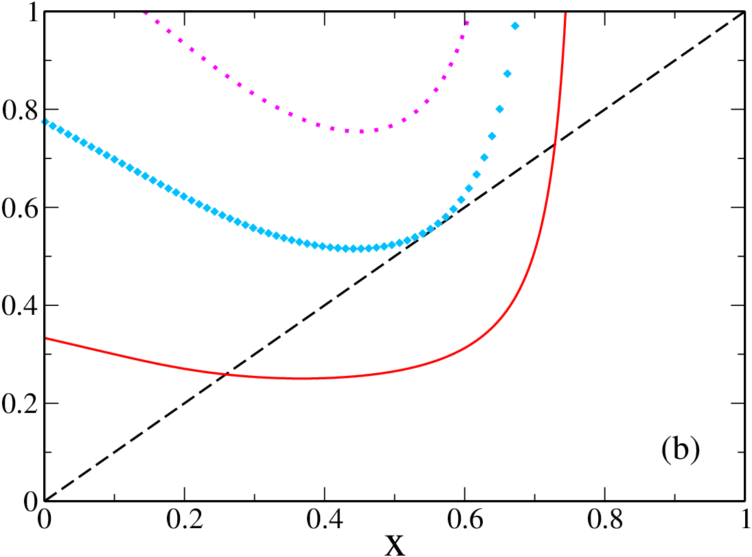
This equation has one, two, or none solutions between and depending on the parameters. Two different solutions correspond to and while a single solution means that does not exist. Moreover if is large enough, there is no solution, which means that there are always available vaccines when needed.
Based on a similar reasoning we can find and for fixed . From Eqs. (28) we can derive a similar expression to Eq. (29) for a Poisson network:
| (30) |
which has two or none solutions depending on .
In Fig. 8 we show the graphical solution of the previous equations for different values of . In (a) we graphically solve Eq. (29) for fixed . For the curve intersects the identity in only one point, which corresponds to . On the contrary for there are two intersection points, which denotes the existence of . For the curve is tangential to the identity, and thus . When there is no solution. Similarly we show in Fig. 8 (b) the solutions of Eq. (29) for fixed . In this case for now we have two intersection points, which correspond to and . For the curve is tangential to the identity and hence there is a single solution, which means . As we can see beyond this point there is no solution.

Appendix E Supplementary figures of the steady state
In Fig. 9 we show how the steady state changes when the recovery time is greater than . Note that this figure is similar to Fig. 5, with the same vaccination probability , vaccination limits and , and a different recovery time . We see that , unlike which barely changes, is lower than for . Furthermore, because the individuals are infected during a larger period of time, the fraction of recovered is larger and so is the discontinuous jump.
On the other hand in Fig. 10 (a) we show the fracion of vaccinated and recovered individuals in the steady state as a function of the infection probability , for a network with a power law degree distribution, and for different vaccination probabilities . The vaccination limit and the recovery time are fixed, and . We observe that for low values of the curves of vaccinated individuals exhibit a maximum while, for larger values they are monotonically increasing. As explained in the main text, exists as long as the curve of vaccinated individuals has a maximum, hence in this case for only exists. In addition, in Fig. 10 (b) we show the fraction of recovered individuals, which as expected decrease when the vaccination probability is higher.


References
- [1] S. Boccaletti, V. Latora, Y. Moreno, M. Chavez, and D. Hwang, Phys. Rep. 424, 175 (2006).
- [2] A. Barrat, M. Barthélemy, R. Pastor-Satorras, and A. Vespignani, Proc. Natl. Acad. Sci. USA 101, 3747 (2004).
- [3] M. E. J. Newman, Networks: An Introduction (Oxford University Press, 2010).
- [4] R. Cohen and S. Havlin, Complex Networks: Structure, Robustness and Function (Cambridge University Press, 2010).
- [5] C. Cattuto, W. V. den Broeck, A. Barrat, V. Colizza, J.-F. Pinton, and A. Vespignani, PLoS ONE 5, e11596 (2010).
- [6] M. C. Gonzalez, C. A. Hidalgo, and A.-L. Barabasi, Nature 453, 779 (2008).
- [7] J. Gómez-Gardeñes, V. Latora, Y. Moreno, and E. Profumo, Proceedings of the National Academy of Sciences 105, 1399 (2008).
- [8] E. M. Volz, J. C. Miller, A. Galvani, and L. A. Meyers, PLoS Comput. Biol. 7, e1002042 (2011).
- [9] N. T. J. Bailey, The Mathematical Theory of Infectious Diseases (Griffin, London, 1975).
- [10] R. M. Anderson and R. M. May, Infectious Diseases of Humans: Dynamics and Control (Oxford University Press, Oxford, 1992).
- [11] R. Pastor-Satorras and A. Vespignani, Phys. Rev. E 65, 036104 (2002).
- [12] M. De Domenico, C. Granell, M. A. Porter, and A. Arenas, Nature Physics 12 (2016).
- [13] C. Castellano and R. Pastor-Satorras, Phys. Rev. Lett 105, 218701 (2010).
- [14] R. Pastor-Satorras, C. Castellano, P. Van Mieghem, and A. Vespignani, Rev. Mod. Phys. 87, 925 (2015).
- [15] W. Wang, M. Tang, H. E. Stanley, and L. A. Braunstein, Reports on Progress in Physics 80, 036603 (2017).
- [16] R. Cohen, S. Havlin, and D. ben-Avraham, Phys. Rev. Lett. 91, 247901 (2003).
- [17] L. K. Gallos, F. Liljeros, P. Argyrakis, A. Bunde, and S. Havlin, Phys. Rev. E 75, 045104 (2007).
- [18] Z. Wang, C. T. Bauch, S. Bhattacharyya, A. d’Onofrio, P. Manfredi, M. Perc, N. Perra, M. Salathé, and D. Zhao, Physics Reports 664, 1 (2016).
- [19] L. D. Valdez, P. A. Macri, and L. A. Braunstein, Physica A: Statistical Mechanics and its Applications 392, 4172 (2013).
- [20] L. Wang, Y. Zhang, T. Huang, and X. Li, Phys. Rev. E 86, 032901 (2012).
- [21] M. E. J. Newman, Phys. Rev.E 66, 016128 (2002).
- [22] Y. Moreno, R. Pastor-Satorras, and A. Vespignani, The European Physical Journal B-Condensed Matter and Complex Systems 26, 521 (2002).
- [23] E. Volz, Journal of mathematical biology 56, 293 (2008).
- [24] J. C. Miller, Journal of mathematical biology 62, 349 (2011).
- [25] V. Colizza, A. Barrat, M. Barthélemy, and A. Vespignani, Proceedings of the National Academy of Sciences 103, 2015 (2006).
- [26] L. A. Meyers, B. Pourbohloul, M. E. Newman, D. M. Skowronski, and R. C. Brunham, Journal of theoretical biology 232, 71 (2005).
- [27] L. D. Valdez, P. A. Macri, and L. A. Braunstein, PLOS ONE 7, 1 (2012a).
- [28] E. Volz and L. A. Meyers, Proceedings of the Royal Society of London B: Biological Sciences 274, 2925 (2007).
- [29] C. Xia, L. Wang, S. Sun, and J. Wang, Nonlinear Dynamics 69, 927 (2012).
- [30] C. Buono, L. G. Alvarez-Zuzek, L. A. Braunstein, and P. A. Macri, PLOS ONE 9, e92200 (2014).
- [31] C. Buono and L. A. Braunstein, EPL (Europhysics Letters) 109, 26001 (2015).
- [32] L. G. Alvarez-Zuzek, H. E. Stanley, and L. A. Braunstein, Scientific Reports 5, 12151 (2015a).
- [33] C. Lagorio, M. Dickison, F. Vazquez, L. A. Braunstein, P. A. Macri, M. V. Migueles, S. Havlin, and H. E. Stanley, Phys. Rev. E 83, 026102 (2011).
- [34] L. G. Alvarez-Zuzek, C. Buono, and L. A. Braunstein, in Journal of Physics Conference Series, Vol. 640 (2015) p. 012007.
- [35] L. D. Valdez, P. A. Macri, and L. A. Braunstein, Phys. Rev. E 85, 036108 (2012b).
- [36] L. D. Valdez, H. H. Aragão Rêgo, H. E. Stanley, and L. A. Braunstein, Sci. Rep. 5, 12172 (2014).
- [37] M. F. C. Gomes, A. Pastore y Piontti, L. Rossi, D. Chao, I. Longini, M. E. Halloran, and A. Vespignani, PLOS Current Outbreaks (2014).
- [38] P. S. Gsell, A. Camacho, A. J Kucharski, C. H Watson, A. Bagayoko, S. V. Danmadji Nadlaou, et al., The Lancet Infectious Diseases 17, 1276 (2017).
- [39] F. Fenner, D. A. Henderson, I. Arita, Z. Jezek, and I. D. Ladnyi, Smallpox and its eradication (World Health Organization, 1988).
- [40] A. Lokhov, Y. and D. Saad, Proceedings of the National Academy of Sciences 14, 8138 (2017).
- [41] G. Tragler, J. P. Caulkins, and G. Feichtinger, Operations Research 49, 325 (2001).
- [42] J. C. Miller, A. C. Slim, and E. M. Volz, Journal of the Royal Society Interface 9, 890 (2012).
- [43] L. Bötcher, O. Woolley-Meza, N. A. Araújo, H. J. Herrmann, and D. Helbing, Scientific Reports 5, 16571 (2015).
- [44] X. Chen, T. Zhou, L. Feng, J. Liang, F. Liljeros, S. Havlin, and Y. Hu, ArXiv e-prints (2016), arXiv:1611.00212 [physics.soc-ph] .
- [45] X. Chen, R. Wang, M. Tang, S. Cai, H. E. Stanley, and L. A. Braunstein, New Journal of Physics 20, 013007 (2018).
- [46] L. G. Alvarez-Zuzek, M. A. Di Muro, S. Havlin, and L. A. Braunstein, ArXiv e-prints (2018), arXiv:1804.10593 [physics.soc-ph] .
- [47] M. E. J. Newman, S. H. Strogatz, and D. J. Watts, Phys. Rev. E 64, 026118 (2001).
- [48] M. E. J. Newman, Phys. Rev. E 67, 026126 (2003).
- [49] M. Molloy and B. Reed, Random Structures and Algorithms 6, 161 (1995).
- [50] R. Cohen, K. Erez, D. ben-Avraham, and S. Havlin, Phys. Rev. Lett. 85, 4626 (2000).
- [51] R. Parshani, S. V. Buldyrev, and S. Havlin, Proc. Natl. Acad. Sci. 108, 1007 (2011).
- [52] D. Zhou, A. Bashan, R. Cohen, Y. Berezin, N. Shnerb, and S. Havlin, Phys. Rev. E 90, 012803 (2014).
- [53] D. S. Callaway, M. E. J. Newman, S. H. Strogatz, and D. J. Watts, Phys. Rev. Lett. 85, 5468 (2000).
- [54] F. Velásquez-Rojas and F. Vazquez, Physical Review E 95, 052315 (2017).
- [55] J. Gómez-Gardeñes, L. Lotero, S. Taraskin, and F. Pérez-Reche, Scientific reports 6, 19767 (2016).