The Distribution and Excitation of CH3CN in a Solar Nebula Analog
Abstract
Cometary studies suggest that the organic composition of the early Solar Nebula was rich in complex nitrile species such a CH3CN. Recent ALMA detections in protoplanetary disks suggest that these species may be common during planet and comet formation, but connecting gas phase measurements to cometary abundances first requires constraints on formation chemistry and distributions of these species. We present here the detection of seven spatially resolved transitions of CH3CN in the protoplanetary disk around the T-Tauri star TW Hya. Using a rotational diagram analysis we find a disk-averaged column density of NT=1.45 cm-2 and a rotational temperature of Trot=32.7 K. A radially resolved rotational diagram shows the rotational temperature to be constant across the disk, suggesting that the CH3CN emission originates from a layer at z/r0.3. Through comparison of the observations with predictions from a disk chemistry model, we find that grain-surface reactions likely dominate CH3CN formation and that in situ disk chemistry is sufficient to explain the observed CH3CN column density profile without invoking inheritance from the protostellar phase. However, the same model fails to reproduce a Solar System cometary abundance of CH3CN relative to H2O in the midplane, suggesting that either vigorous vertical mixing or some degree of inheritance from interstellar ices occurred in the Solar Nebula.
I Introduction
a Observations of comets and meteorites show that the planet and comet forming midplane of the young Solar Nebula had a rich organic volatile composition [45, e.g.,]. ALMA observations and the recent Rosetta mission have both explicitly shown that comets are abundant in nitrile species such as HCN and CH3CN [17, 39, e.g.,]. Tracing the chemistry of this family of organic molecules is of particular interest, as HCN and related nitriles are the starting point for the eventual synthesis of important bio-molecules such as glycine [9, 48, 49, 47, e.g.,].
In the protoplanetary disks where other planetary systems are just starting to form, the smallest nitriles CN and HCN have long been well-known [21, 60, e.g.,]. Larger nitriles such as HC3N have only been found more recently [13], and ALMA is just now beginning to reveal more complex species such as CH3CN [46, 7]. The provenance of these species in disks is unclear, however, and will play a role in setting their final abundances in the forming cometary bodies. Organics may be directly inherited from the chemically rich protostellar stage [36, e.g.,], formed in situ in the disk [54, 63, e.g.,], or both pathways may contribute. If inheritance from the protostellar stage dominates then nitrile abundances will likely be similar across disks within a given stellar association, while dominant in situ formation may imply that cometary nitrile abundances will be highly disk dependent.
Testing the origin of nitriles such as CH3CN in disks will require constraining their abundances and formation routes, allowing comparison to predictions from the different inheritance scenarios. As CH3CN can efficiently form through both gas-phase and grain-surface reactions, however, resolved observations of the disk abundance distribution are necessary to determine its dominant formation route. Thus far, observational constraints have been sparse [46, 7]. Based on the inferred abundance of CH3CN in MWC 480, [46] concluded that in situ grain surface chemistry must play an important role. This same chemistry should produce CH3CN the disk midplane, affecting the composition of forming comets and planetesimals. Better constraints on the distribution and excitation of CH3CN in disks are therefore crucial to test this hypothesis and connect disk chemistry with cometary measurements.
In this paper we present the detection of seven lines of CH3CN in the disk around TW Hya. A well-studied, old [38, 66, 10 Myr; e.g.,] T Tauri star, TW Hya hosts the closest [40, 59.51 pc;] protoplanetary disk, and is a good analog for the Solar Nebula [53, 6, 0.8 M⊙, spectral type K7; e.g.,]. We present the observations and the details of their reduction and imaging in §2. In §3, we use a rotational diagram analysis to empirically constrain the CH3CN column density and rotational temperature, both disk-averaged and radially resolved, and compare with predictions from detailed chemical models. In §4 we discuss these results and their implications for midplane CH3CN abundances and incorporation into planetesimals and forming comets. A summary is given in §5.
II Observations
II.1 Observational details
| Transition | Symmetry | Frequency | Eu | S | Int. Flux Dens.a | Filter response |
|---|---|---|---|---|---|---|
| (MHz) | (K) | (D2) | (mJy km s-1) | () | ||
| 120–110 | A | 220747.3b | 68.9 | 183.7c | 82 7 | 17.8 |
| 121–111 | E | 220743.0b | 76.0 | 182.5c | 78 7 | 15.9 |
| 122–112 | E | 220730.3b | 97.4 | 178.6c | 41 7 | 7.2 |
| 130–120 | A | 239137.9b | 80.3 | 199.1c | 81 7 | 13.1 |
| 131–121 | E | 239133.3b | 87.5 | 197.9c | 70 7 | 9.3 |
| 132–122 | E | 239119.5b | 108.9 | 194.3c | 28 7 | 5.7 |
| 133–123 | A | 239096.5b | 144.6 | 188.5c | 12 7 | 3.5 |
TW Hya was observed on 29-Dec-2016 and 09-Jan-2017 in Band 6 as part of the ALMA Cycle 4 project 2016.1.01046.S. The first execution block included 43 antennas with projected baseline lengths between 15 and 460 m (11–353 k). The second execution block included 47 antennas with projected baseline lengths between 15 and 384 m (11–295 k). The on-source integration times were 32 and 31 minutes, respectively, for a total on-source integration time of 63 minutes. The correlator setup was identical for both execution blocks and included a Time Division Mode (TDM) continuum window centered at 237 GHz with a bandwidth of 2 GHz as well as Frequency Division Mode (FDM) spectral windows centered at 219.560, 220.740, and 239.112 GHz. These spectral windows had bandwidths of 58.59 MHz and channel spacings of 61 kHz (0.08 km s-1), and they targeted the C18O J=2–1, CH3CN J=12–11, and CH3CN J=13–12 molecular transitions, respectively. As CH3CN is a prolate symmetric top with C3v symmetry its rotational spectrum has a k-ladder structure with two spin symmetry states (A/E), allowing a single set of observations to probe a wide range of upper state energies. We cover three transitions in the J=12–11 k-ladder and four transitions in the J=13–12 k-ladder, tabulated in Table 1. The 123–113 transition was not covered in our spectral setup.
For both executions, the quasar J1058+1033 was used for bandpass calibration and the quasar J1037-2934 was used for phase calibration. Callisto was used as the flux calibrator for the first execution, and Ganymede was used as the flux calibrator for the second execution. We additionally used the disk continuum emission in each execution block to perform three rounds of phase self-calibration and one round of amplitude self-calibration in CASA version 4.3. These solutions were then applied to the spectral line observations.
II.2 Results
The observations were first analyzed using a matched filtering technique for identifying weak line emission, described in [43]. The C18O J=2–1 transition was imaged using CLEAN at the native spectral resolution (61 kHz, 0.08 km s-1) with Briggs weighting (robust=0.5), producing a high SNR image cube (peak SNR=32). This image cube was then used as a filter for the CH3CN spectral windows using the VISIBLE code11 1 VISIBLE is publicly available at https://github.com/AstroChem/VISIBLE. From the resultant filter impulse response spectra we detected all three transitions in the J=12–11 k-ladder covered by the spectral setup and all four transitions in the J=13–12 k-ladder with spectral coverage. The peak filter responses for each transition are given in Table 1.

The seven detected transitions were then individually imaged using CLEAN with natural weighting and a velocity resolution of 0.2 km s-1, centering each image cube on the transition rest frequency. The J=13–12 transitions had a small uv-taper (‘outertaper’ = 035) applied to force the synthesized beam to match that of the J=12–11 transitions (105 083). The rms of the image cubes was 3.2 mJy beam-1 in each channel, and channel maps are presented in Appendix A. Moment-0 maps of the transitions are shown in Fig. 1 and were created by integrating all emission between 2.1–3.7 km s-1 with no clipping threshold.
Deprojected and azimuthally averaged radial intensity profiles (Fig. 2) were calculated from the moment-0 maps in Fig. 1 using an inclination of 7 and PA of 155 [50, 1, 2]. All transitions are centrally peaked, but the beam size is relatively large (50-60 AU) compared to the extent of the emission, leaving open the possibility of a ringed morphology at small radii. The transitions all have similar profile shapes, with their relative strengths decreasing with increasing ka.
Spectra were extracted for each transition using two methods. First, an elliptical mask 35 in diameter was used (line profiles in Fig. 3), which corresponds to a radial extent of 105 AU and encapsulates all emission given the radial profiles in Fig. 2. Second, a Keplerian mask convolved with the synthesized beam was used to extract the shaded profiles in Fig. 3, offering a better estimate of the true flux of each transition. The convolved Keplerian mask was truncated at a radial distance of 105 AU, and thus covers the same total solid angle as the elliptical mask. Flux measurements, listed in Table 1, were made by integrating the Keplerian extracted spectra between 2.1 and 3.7 km s-1. Uncertainty on each flux measurement was determined through bootstrapping, repeating the extraction and integration 10,000 times on an identical number of randomly-selected nearby emission-free channels (sampled with replacement). The standard deviation of these values is reported as the uncertainty on the flux measurement.
III CH3CN column density and excitation temperature
The k-ladder structure of CH3CN’s rotational spectrum allows multiple transitions to be observed simultaneously, spanning a wide range of upper state energies. With this lever arm, the CH3CN column density and excitation temperature can be well-constrained through a rotational diagram analysis [27, e.g.,]. We initially assume local thermodynamic equilibrium (LTE) excitation, as the critical densities of the J=13–12 and J=12–11 CH3CN transitions are 2.6106 and 2.0106 cm-3, respectively, at a typical disk molecular layer temperature of 40K [57, extrapolated to higher J and interpolated in temperature from]. Typical disk gas densities are 1106 cm-3, apart from the upper regions of the disk atmosphere (z/r0.6), which we do not expect these observations to probe.
III.1 Disk-averaged analysis
We first calculate a disk-averaged column density and excitation temperature. Under an assumption of optically thin emission, the column density of molecules in the upper state of each transition, , is related to the emission surface brightness, through the equation:
| (1) |
where is the Einstein coefficient and is the linewidth [12, e.g.,]. The disk-averaged emission intensity is , where is the flux density and is the solid angle subtended by the source. Substituting for and inverting Eq. 1:
| (2) |
is the integrated flux density reported for each transition in Table 1, and we use the total solid angle covered by the beam-convolved Keplerian mask as an estimate of .
Following Gordy & Cook [28], the upper state level population can be related to the total column density by the Boltzmann equation:
| (3) |
where is the degeneracy of the upper state level, is the molecular partition function, is the rotational temperature, and is the upper state energy. CH3CN is a symmetric top with C3v symmetry, and the upper state degeneracy can be written as
| (4) |
where , for , and for , and is the reduced nuclear spin degeneracy. For CH3CN, can be defined as
| (5) |
The partition function can be approximated for a molecule with C3v symmetry as
| (6) |
where is a unitless symmetry parameter, equal to 3 for a molecule with C3v symmetry, and A and B are the molecular rotational constants. Values for these rotational constants and all other spectral line data were taken from the Spectral Line Atlas of Interstellar Molecules (SLAIM)22 2 Available at http://www.splatalogue.net. [51, F.J. Lovas, private communication,].
In a conventional rotational diagram analysis [27, e.g.,], taking the logarithm of Eq. 3 allows for a linear least squares regression:
| (7) |
If the level populations, , are semi-log plotted against the upper state energies, , then the rotational temperature, , and total column density, , can be derived from the best fit slope and intercept, respectively. Under the assumption of optically thin emission, , Eq. 2 can be used to calculate . The optical depth of the observed CH3CN transitions is unknown a priori, however. In the case that the optical depth , an optical depth correction factor must be applied:
| (8) |
and thus the true level populations become
| (9) |
such that Eq. 7 is rewritten as
| (10) |
The optical depths of individual transitions are often directly determined through hyperfine ratios or observations of isotopomers, but can also be related back to the upper state level populations:
| (11) |
can therefore be written as a function of and substituted into Eq. 10 to construct a likelihood function which can then be used for minimization.
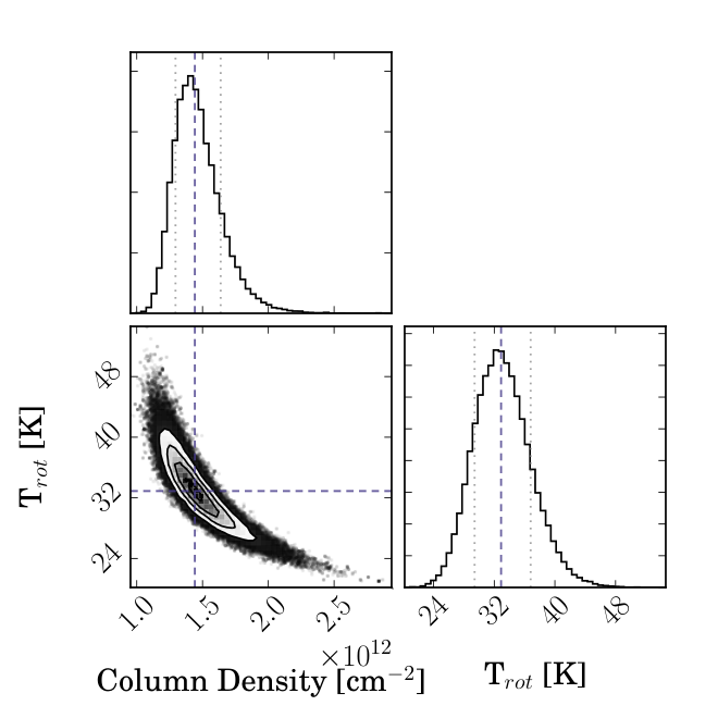
Given this likelihood function, we use the affine-invariant Markov chain Monte Carlo (MCMC) code emcee [25] to fit the data and generate posterior probability distributions of both and (see Fig. 12 in Appendix B). These probability density functions describe the range of possible column densities and rotational temperatures that are consistent with our observed data. Random draws from these posteriors are plotted in blue in Fig. 4, with corrected values of plotted against . We find a disk-averaged column density of NT=1.45 cm-2 and a rotational temperature of Trot=32.7 K, where parameters and uncertainties are listed as the 50th, 16th, and 84th percentiles from the marginalized posterior distributions, respectively. Corresponding values of range between 0.002–0.012, confirming that these transitions of CH3CN are optically thin. These values show a good fit to both the complete dataset as well as the individual J=12–11 and J=13–12 k-ladders (shown in orange and red, respectively), consistent with the assumption of LTE excitation.
III.2 Radially resolved analysis
As the observed CH3CN transitions are strongly detected and moderately resolved (with a beam size of 50 AU), NT and Trot can be further constrained as a function of radius. We repeat the rotational diagram analysis previously described, but now use intensities from the radial profiles of each transition from Fig. 2 rather than disk-averaged intensities. Posterior distributions for NT and Trot are calculated at intervals of 1 AU and are plotted in Fig. 5. The rotational diagrams (not shown) remain log-linear and well-behaved out to 70 AU but become non-linear exterior to this distance, leading to the large uncertainties in Trot.
The observed NT profile decreases with radius from 5 to 0.9 cm-2. This is consistent with the disk-averaged column density of NT=1.45 cm-2, which is overplotted in red in Fig. 5. The disk-averaged column density is biased towards the low end of the radially resolved column density range. The majority of the emission (and therefore molecular column) is concentrated in the inner regions of the disk (R50 AU) and the disk-averaged intensities (integrated out to R=105 AU) are therefore diluted. Trot shows a flat radial profile, ranging between 30–34 K, consistent with the disk-averaged rotation temperature, Trot=32.7 K.
III.3 Comparison to chemical models
We compare the empirical contraints derived in §3.1 and §3.2 to the predictions of a time-dependent chemical model [24, 14] evolved for 1 Myr. The assumed density and temperature structures, constrained by the TW Hya SED and previous HD observations [6] in [15], are shown in Fig. 6 panels a and b, respectively. The initial chemical abundances of the model, listed in Table 2, are based on values from [15] but with updated CO and H2O depletion factors. CO is depleted by a factor of 20 to approximately compensate for the known carbon depletion in TW Hya [23, 37, 55, e.g.]. H2O is depleted in the model by a factor of 100 [19, e.g.]. No CH3CN is included in the initial abundances, and thus all CH3CN in the model is produced in situ. The FUV and X-ray radiation fields within the disk (Fig. 6, panels c,d) were calculated using the Monte Carlo code and cross sections from [11], the observed TW Hya FUV spectrum [32, 33], and a best-fit X-ray model for TW Hya from [15]. A reduced cosmic ray ionization rate was assumed, as TW Hya has been found to have a reduced cosmic ray ionization rate due to exclusion either by winds or magnetic fields [15, s-1; SSX model;].

| Species | Abundancea | Species | Abundancea |
|---|---|---|---|
| H2 | He | ||
| N2 | CO | ||
| H2O(gr) | H | ||
| HCO+ | C2H | ||
| CS | SO | ||
| C+ | Si+ | ||
| Mg+ | Fe+ |
The chemical reaction network contains a total of 5970 reactions and 600 species. Within this network, three reactions are primarily responsible for the formation of CH3CN [63, 62]. In the gas phase, formation occurs through the radiative association reaction [31]
| (12) |
followed by dissociative recombination
| (13) |
It should be noted, however, that the implicit isomerization of CH3NCH+ to CH3CNH+ in Eq. 12 as written would likely require a three-body interaction to be efficient [3, e.g.] and is not firmly established in the literature as a viable process at the low densities present in protoplanetary disks. An analogous reaction for HNC is also possible
| (14) |
with a disk-integrated HNC/HCN ratio of 0.1-0.2 having been previously measured for TW Hya [29]. Destruction pathways for gas-phase CH3CN include UV photodissociation into CH3 + CN and reactions with C+.
On grain surfaces, there are two viable formation pathways through a Langmuir-Hinshelwood mechanism: (1) sequential hydrogenation of C2N or (2) a neutral-neutral grain surface reaction between CH3 and CN [61, 63]. A reactive desorption efficiency of 1% and a photodesorption yield of 10-3 were assumed, with an additional assumption that the CH3CN molecule always desorbs intact. The validity of these assumptions and their impact are discussed in more detail in §4.1.3. Thermal desorption and freeze-out in the model are treated using the Polyani-Wigner relation, with an assumed binding energy of 4680 K for CH3CN [16].
To isolate the respective contributions of gas phase and grain-surface formation mechanisms, we ran the chemical model twice, once with grain-surface reactions turned on and once with them turned off. Fig. 7 shows the resultant gas phase CH3CN abundance profiles (panels a,b). Both gas phase and grain-surface reactions contribute to the total CH3CN reservoir, but form distinct vertical layers. Gas phase reactions produce CH3CN in a layer at z/r 0.5, where the gas temperature is 50 K. The upper boundary of this layer sits along the FUV =1 surface, and is primarily set by the UV photo-dissociation of CH3CN. The lower boundary is set where the reactant CH is no longer formed in appreciable quantities due to the FUV and X-ray optical depths. Grain-surface reactions meanwhile produce a layer of CH3CN in the gas phase at z/r 0.3 (Tgas 35 K), with formation dominated by sequential C2N hydrogenation. C2N is primarily formed in the gas phase through the reaction
| (15) |
and then freezes out onto grain surfaces. The upper boundary of the grain-surface CH3CN layer is set by this freeze-out of C2N and the lower boundary is set by high optical depths limiting photodesorption of CH3CN off the grain surfaces.

The model abundance profiles were vertically integrated to calculate column density profiles (Fig. 7 panels c,d). The model column density profiles, shown in black, were then convolved with the synthesize beam of the observations to produce the smoothed profiles shown in red. From these profiles, it is clear that grain-surface contributions in the full network model increase the integrated column density by a factor of 4–10 across the disk. Comparing the beam smoothed model profiles with the observed column density profile in Fig. 5, we find that gas phase reactions alone are insufficient to reproduce the observed column densities, while inclusion of grain-surface reactions reproduces the observed column densities within a factor of 2 across the disk.
Although the beam smoothed profiles allow a rough comparison to our best fit observed column density profile, a more detailed comparison requires an identical analysis procedure for both the observations and chemical model results. We therefore used the chemical model output to calculate simulated emission profiles for the observed CH3CN transitions using the radiative transfer code RADMC-3D [20]. A distance of 59.5 pc, PA of 155, and stellar mass of 0.8 M⊙ (to determine line broadening) were assumed for the radiative transfer [38, 50, 1, 2]. An inclination of 8 was assumed, which approximately accounts for the slight warp in the TW Hya disk [52] and was found to fit our observations relatively well (see Appendix A). Simulated ALMA observations were then calculated for each transition using the vissample package [43] and the antenna configuration of the original observations.
From these simulated observations, we repeated the analysis described in §3.1 and calculated a disk-averaged rotational temperature and column density, overplotted in dashed black in Fig. 4. The disk-averaged calculated column density of NT=1.491012 cm-2 and rotational temperature of Trot=36.6 K both agree with the observed column density of NT=1.451012 cm-2 and rotational temperature of Trot=32.7 K within the errors.
Similarly, we extracted deprojected and azimuthally-averaged radial intensity profiles and repeated the analysis described in §3.2 to calculate resolved column density and rotational temperature profiles, overplotted in dashed black in Fig. 5. Both profiles match the observations relatively well. The model rotational temperature profile is up to 15 K warmer than the observations however, especially at radii 50 AU. This might be expected given the distribution of CH3CN seen in Fig. 7, panel a, peaking at small radii and in a temperature layer 50 K. This point is discussed further in §4.1.
IV Discussion
IV.1 CH3CN abundance structure and formation chemistry
IV.1.1 Insights from observations
A rotational diagram analysis of our observations shows that CH3CN in TW Hya emits at a near constant temperature of 30–35 K across the disk. From our assumed physical model of TW Hya, this temperature suggests emission from a vertical layer at z/r0.3. These first observational constraints on the vertical distribution of CH3CN are in good qualitative agreement with the layered CH3CN distribution predicted by the chemical models in [46]. Similarly, we find that our observed radial column density profile is in good qualitative agreement with the predictions of [63] and the observational results of [46], which both found column density profiles between 1012–1013 cm-2 that monotonically decreased with radius.
IV.1.2 Comparison of chemical models and observations
We attempted to gain an intuition for the dominant CH3CN formation pathway by comparing these observational results with two chemical models, with and without grain-surface chemistry. The full chemical network predicts emission which is in remarkably good agreement with our observations, especially given that the model has not been adjusted in any manner to match the data. The model with no grain-surface reactions underpredicts our measured fluxes by over an order of magnitude, suggesting that grain-surface formation of CH3CN may be the main in situ formation pathway. We additionally find that at all times in the full-network model, the total grain-surface formation rate dominates over the gas-phase formation rate by factors of 2-10. Dominant grain-surface formation is further supported by our observed temperature layer (30–35 K, z/r0.3) being better matched to the grain-surface formation layer than the gas-phase formation layer in Fig. 7. The limited spatial resolution of our observations and the caveats of our chemical model presented in §4.1.3, however, prevent a more robust quantitative analysis of the relative gas-phase and grain-surface contributions.
Although the full network model predicts adequate integrated fluxes, some differences remain between the model and observations. First, the radial profile of the model column density is slightly more centrally peaked (even after beam convolution) than the observed column density profile (Figs. 5 and 7). Second, although the best-fit disk-averaged column density and rotational temperature are well-matched between the model and observations, the radially resolved model temperature profile is up to 15 K warmer than the observed temperature profile.
These differences are inherently linked; a more centrally peaked column density results in more emission at small radii, where the gas temperature is higher for a given z/r. A number of phenomena therefore could possibly explain these discrepancies. First, a central depletion in the CH3CN emission cannot be ruled out by our observations, given their relatively low spatial resolution. By stacking the observations and examining the resultant channel maps, we are able to constrain the possible radial extent of such a feature to be less than 16 AU (see Appendix A). Second, the chemical model may over-estimate gas-phase CH3CN production, resulting in an enhanced contribution of warm (50 K) CH3CN at small radii. Third, the temperature of the CH3CN emission is likely sensitive to our assumptions about the physical structure of TW Hya and its FUV and X-ray radiation fields in particular, as the boundaries of the CH3CN layer are directly linked to the optical depths of the radiation fields (see §3.3). High resolution observations of smaller molecules such as HCN may allow future model refinement by anchoring the assumed initial conditions and disk physical characteristics.
IV.1.3 Chemical model assumptions and caveats
A number of assumptions made in our chemical modeling complicate our interpretation of both the observations and models. First, molecules larger than CH3CN are not included in the model and CH3CN likely acts as a chemical ‘sink’, enhancing model abundances. Second, given the uncertainties associated with the dominant gas-phase reaction (see §3.3), it is unclear to what extent this pathway contributes to the observed CH3CN abundance. If the assumed efficiency of this reaction in the model is too high, this may partially explain the higher rotational temperature found for the model compared to the data. Third, we assumed that CH3CN is always able to photodesorb intact from grain-surfaces. Recent investigation on CH3OH photodesorption suggests that larger molecules such as CH3CN fragment and thus may have difficulty efficiently photodesorbing intact from grain surfaces [10, 18, 64]. If this is the case, reactive desorption may play a larger role as a mechanism for non-thermal CH3CN desorption. Finally, our model initial conditions assume flat depletion of CO and H2O across the disk. In reality, spatial variations in depletion and sequestration will result in a modified C/O ratio, which in turn will affect CH3CN abundances. In particular, the formation of cyanides such as CH3CN has been shown to be sensitive to carbon and oxygen abundances, with an enhanced C/O ratio resulting in more efficient cyanide formation [19]. The expected nitrile enhancements for older disks with grain growth and radial drift have been tentatively observed by [30], and a similar effect was invoked by [5] to explain hydrocarbon rings around TW Hya.
IV.2 Implications for cometary CH3CN abundances
Our observations probe gas-phase abundances at a vertical layer in the disk of z/r0.3. In contrast, comets form in the disk midplane and their bulk compositions are primarily set by grain-surface chemical abundances, rather than gas-phase abundances. Interpreting the implications of our observations for the chemical composition of comets therefore requires extrapolation to the disk midplane through our chemical model. Fig. 8 panels a,b show the grain-surface abundances of CH3CN in our chemical models with grain-surface chemistry turned on and off, respectively. Although no CH3CN is formed on grain-surfaces in the latter model, freeze-out still results in a non-negligible CH3CN grain-surface abundance.
To compare these grain-surface abundances to measured cometary CH3CN abundances in the Solar System [45, 10-4 relative to H2O, e.g.,], panels c,d of Fig. 8 show CH3CN(gr)/H2O(gr) abundance ratios across the disk model. Initial H2O(gr) abundances in the midplane are inherited from the protostellar phase. We correct for the depletion factor assumed for gas-phase H2O in the disk surface [19, e.g.](see §3.3), as ices in the disk midplane are not expected to be depleted. Gas-phase reactions alone (Fig. 8, panel d) are clearly insufficient to reproduce cometary CH3CN abundances 710-5–310-4 [45, e.g.,] near the midplane (ie z/r0.1). Incorporation of grain-surface reactions (Fig. 8, panel c), however, produces abundances closer to cometary values (up to 510-4) in the comet forming regions of the disk (R10–30 AU), consistent with the results of [63].

Fig. 9 plots CH3CN(gr)/H2O(gr) ratios as a function of z/r at a variety of radii in the disk, comparing these values to the range of known cometary CH3CN(gr)/H2O(gr) ratios. In situ formation in the comet forming zone (R10–30 AU) is insufficient to produce cometary abundances of CH3CN at the midplane, but can easily yield these abundances at slightly higher disk layers (z/r0.04), especially at smaller radii. A detailed understanding of the coupling between chemistry and vertical motion of material within the disk will be necessary to determine if CH3CN produced higher in the disk can be efficiently transported to the midplane for incorporation into comets [56, 26, e.g.,]. In particular, such an analysis would require chemical modeling which incorporates both dust settling and turbulent diffusion, as these phenomena have pronounced effects on CH3CN abundance distributions and the coupling between gas-phase and grain surface abundances [56, 46, e.g.,].
We note that the CH3CN(gr)/H2O(gr) ratios shown in Fig. 9 are lower limits, as no inheritance from the protostellar stage is included in our models. Chemical modeling in [22] suggests that such inheritance is possible, with interstellar ices abundances preserved in environments which are shielded from cosmic rays [15, e.g., TW Hya,]. Observational evidence for protostellar inheritance of CH3CN is mixed, however. [46] find CH3CN/HC3N/HCN ratios in MWC 480 that are inconsistent with those found in protostellar regions such as IRAS 16293-2422 [59, e.g.,], while [7] find CH3CN/HC3N ratios in a number of disks which are consistent with protostellar values.
The detection of CH3CN around TW Hya offers an additional opportunity to evaluate the possibility of protostellar inheritance, as this is the only disk where CH3OH has been detected thus far [65]. We find an approximate CH3CN/CH3OH column density ratio of unity, which is substantially higher than the few percent found in comets and around protostars [45, 8]. As discussed in [7], two scenarios could explain this finding: a higher photodesorption efficiency for CH3CN than CH3OH (where both species could either be inherited from the protostellar stage or form through in situ grain surface chemistry), or gas phase production of nitriles such as CH3CN could be enhanced by a high C/O ratio as discussed in §4.1.3. Thus although our observations are inconsistent with preserved interstellar abundance ratios, it is possible that inheritance contributes to the total CH3CN abundance in TW Hya.
V Summary
In summary, we have detected emission from seven transitions of CH3CN toward TW Hya. A disk-averaged rotational analysis finds a column density of NT=1.82 cm-2 and a rotational temperature of Trot=29.3 K, and a radially resolved analysis shows this temperature to be flat across the disk. We interpret these results to suggest that CH3CN emission originates from a layer at z/r0.3 throughout the disk. Comparing these observations with the results of a disk chemistry model, we suggest that grain-surface reactions likely dominate CH3CN formation. In situ formation in the model is sufficient to explain observed CH3CN fluxes, although further model refinement is necessary to accurately reproduce CH3CN radial and vertical abundance profiles. Finally, we examine the CH3CN(gr)/H2O(gr) ratio predicted by our model and find that cometary abundances of CH3CN are not present in the disk midplane, but can be found in slightly higher disk layers (z/r0.04), suggesting that inheritance, dust settling, turbulent mixing, or a combination of these effects is necessary to replicate cometary CH3CN abundances in the disk midplane.
References
- [1] Andrews, S. M., Wilner, D. J., Hughes, A. M., et al. 2012, ApJ, 744, 162
- [2] Andrews, S. M., Wilner, D. J., Zhu, Z., et al. 2016, ApJ, 820, L40
- [3] Anicich, V. G., Sen, A. D., McEwan, M. J., & Smith, S. C. 1994, J. Chem. Phys., 100, 5696
- [4] Astropy Collaboration, Robitaille, T. P., Tollerud, E. J., et al. 2013, A&A, 558, A33
- [5] Bergin, E. A., Du, F., Cleeves, L. I., et al. 2016, ApJ, 831, 101
- [6] Bergin, E. A., Cleeves, L. I., Gorti, U., et al. 2013, Nature, 493, 644
- [7] Bergner, J. B., Guzmán, V. G., Öberg, K. I., Loomis, R. A., & Pegues, J. 2018, ApJ, 857, 69
- [8] Bergner, J. B., Öberg, K. I., Garrod, R. T., & Graninger, D. M. 2017, ApJ, 841, 120
- [9] Bernstein, M. P., Dworkin, J. P., Sandford, S. A., Cooper, G. W., & Allamandola, L. J. 2002, Nature, 416, 401
- [10] Bertin, M., Romanzin, C., Doronin, M., et al. 2016, ApJ, 817, L12
- [11] Bethell, T. J., & Bergin, E. A. 2011, ApJ, 740, 7
- [12] Bisschop, S. E., Jørgensen, J. K., Bourke, T. L., Bottinelli, S., & van Dishoeck, E. F. 2008, A&A, 488, 959
- [13] Chapillon, E., Dutrey, A., Guilloteau, S., et al. 2012, ApJ, 756, 58
- [14] Cleeves, L. I., Bergin, E. A., & Adams, F. C. 2014, ApJ, 794, 123
- [15] Cleeves, L. I., Bergin, E. A., Qi, C., Adams, F. C., & Öberg, K. I. 2015, ApJ, 799, 204
- [16] Collings, M. P., Anderson, M. A., Chen, R., et al. 2004, MNRAS, 354, 1133
- [17] Cordiner, M. A., Remijan, A. J., Boissier, J., et al. 2014, ApJ, 792, L2
- [18] Cruz-Diaz, G. A., Martín-Doménech, R., Muñoz Caro, G. M., & Chen, Y.-J. 2016, A&A, 592, A68
- [19] Du, F., Bergin, E. A., & Hogerheijde, M. R. 2015, ApJ, 807, L32
- [20] Dullemond, C. P., Juhasz, A., Pohl, A., et al. 2012, RADMC-3D: A multi-purpose radiative transfer tool, Astrophysics Source Code Library, , , ascl:1202.015
- [21] Dutrey, A., Guilloteau, S., & Guelin, M. 1997, A&A, 317, L55
- [22] Eistrup, C., Walsh, C., & van Dishoeck, E. F. 2016, A&A, 595, A83
- [23] Favre, C., Cleeves, L. I., Bergin, E. A., Qi, C., & Blake, G. A. 2013, ApJ, 776, L38
- [24] Fogel, J. K. J., Bethell, T. J., Bergin, E. A., Calvet, N., & Semenov, D. 2011, ApJ, 726, 29
- [25] Foreman-Mackey, D., Hogg, D. W., Lang, D., & Goodman, J. 2013, PASP, 125, 306
- [26] Furuya, K., & Aikawa, Y. 2014, ApJ, 790, 97
- [27] Goldsmith, P. F., & Langer, W. D. 1999, ApJ, 517, 209
- [28] Gordy, W., & Cook, R. L. 1984, Microwave molecular spectra, [3rd ed.] edn. (New York : Wiley), ”A Wiley-Interscience Publication.”. http://uclibs.org/PID/109941
- [29] Graninger, D., Öberg, K. I., Qi, C., & Kastner, J. 2015, ApJ, 807, L15
- [30] Guzmán, V. V., Öberg, K. I., Huang, J., Loomis, R., & Qi, C. 2017, ApJ, 836, 30
- [31] Herbst, E. 1985, Astrophysical Journal, 291, 226
- [32] Herczeg, G. J., Linsky, J. L., Valenti, J. A., Johns-Krull, C. M., & Wood, B. E. 2002, ApJ, 572, 310
- [33] Herczeg, G. J., Wood, B. E., Linsky, J. L., Valenti, J. A., & Johns-Krull, C. M. 2004, ApJ, 607, 369
- [34] Hunter, J. D. 2007, Computing in Science Engineering, 9, 90
- [35] Jones, E., Oliphant, T., Peterson, P., et al. 2001–, SciPy: Open source scientific tools for Python, , . http://www.scipy.org/
- [36] Jørgensen, J. K., van der Wiel, M. H. D., Coutens, A., et al. 2016, A&A, 595, A117
- [37] Kama, M., Bruderer, S., Carney, M., et al. 2016, A&A, 588, A108
- [38] Kastner, J. H., Zuckerman, B., Weintraub, D. A., & Forveille, T. 1997, Science, 277, 67
- [39] Le Roy, L., Altwegg, K., Balsiger, H., et al. 2015, A&A, 583, A1
- [40] Lindegren, L., Lammers, U., Bastian, U., et al. 2016, A&A, 595, A4
- [41] Loomis, R., Öberg, K., Andrews, S., et al. 2018a, VISIBLE: VISIbility Based Line Extraction, v0.1.0, Zenodo, doi:10.5281/zenodo.1174549. https://doi.org/10.5281/zenodo.1174549
- [42] —. 2018b, VISIBLE: VISIbility Based Line Extraction, , , ascl:1802.006
- [43] Loomis, R. A., Öberg, K. I., Andrews, S. M., et al. 2018c, ArXiv e-prints, arXiv:1803.04987
- [44] McMullin, J. P., Waters, B., Schiebel, D., Young, W., & Golap, K. 2007, in Astronomical Society of the Pacific Conference Series, Vol. 376, Astronomical Data Analysis Software and Systems XVI, ed. R. A. Shaw, F. Hill, & D. J. Bell, 127
- [45] Mumma, M. J., & Charnley, S. B. 2011, ARA&A, 49, 471
- [46] Öberg, K. I., Guzmán, V. V., Furuya, K., et al. 2015, Nature, 520, 198
- [47] Patel, B. H., Percivalle, C., Ritson, D. J., D., D., & Sutherland, J. D. 2015, Nat Chem, 7, 301, article. http://dx.doi.org/10.1038/nchem.2202
- [48] Powner, M. W., Gerland, B., & Sutherland, J. D. 2009, Nature, 459, 239
- [49] Powner, M. W., Sutherland, J. D., & Szostak, J. W. 2010, Journal of the American Chemical Society, 132, 16677, pMID: 21043502. http://dx.doi.org/10.1021/ja108197s
- [50] Qi, C., Ho, P. T. P., Wilner, D. J., et al. 2004, ApJ, 616, L11
- [51] Remijan, A. J., Markwick-Kemper, A., & ALMA Working Group on Spectral Line Frequencies. 2007, in Bulletin of the American Astronomical Society, Vol. 39, American Astronomical Society Meeting Abstracts, 963
- [52] Rosenfeld, K. A., Qi, C., Andrews, S. M., et al. 2012, ApJ, 757, 129
- [53] Rucinski, S. M., & Krautter, J. 1983, A&A, 121, 217
- [54] Sakai, N., Sakai, T., Hirota, T., et al. 2014, Nature, 507, 78
- [55] Schwarz, K. R., Bergin, E. A., Cleeves, L. I., et al. 2016, ApJ, 823, 91
- [56] Semenov, D., & Wiebe, D. 2011, ApJS, 196, 25
- [57] Shirley, Y. L. 2015, PASP, 127, 299
- [58] van der Walt, S., Colbert, S. C., & Varoquaux, G. 2011, Computing in Science Engineering, 13, 22
- [59] van Dishoeck, E. F., Blake, G. A., Jansen, D. J., & Groesbeck, T. D. 1995, ApJ, 447, 760
- [60] van Zadelhoff, G.-J., van Dishoeck, E. F., Thi, W.-F., & Blake, G. A. 2001, A&A, 377, 566
- [61] Wakelam, V., Herbst, E., & Selsis, F. 2006, A&A, 451, 551
- [62] Wakelam, V., Loison, J.-C., Herbst, E., et al. 2015, ApJS, 217, 20
- [63] Walsh, C., Millar, T. J., Nomura, H., et al. 2014, A&A, 563, A33
- [64] Walsh, C., Vissapragada, S., & McGee, H. 2017, ArXiv e-prints, arXiv:1710.01219
- [65] Walsh, C., Loomis, R. A., Öberg, K. I., et al. 2016, ApJ, 823, L10
- [66] Weinberger, A. J., Anglada-Escudé, G., & Boss, A. P. 2013, ApJ, 762, 118
Appendix A Channel Maps
Channel maps of the observed CH3CN transitions are shown in Figs. 10 and 11, generated from the image cubes described in §2 at 0.2 km s-1. Residuals after subtracting the synthesized observations from the full network chemical model described in §3.3 are shown in the figures as well, alternating rows with the observations. Although these residuals are small, a trend is seen where the model over-produces emission in the central channels and under-produces emission at 0.4 km s-1. This can likely be attributed to the small deviation from Keplerian rotation at small radii in TW Hya [52], which we only partially able to account for by slightly increasing the overall inclination of our model (from 6 to 8).
To investigate the distribution of CH3CN at small radii, we additionally stacked the transitions within each k-ladder to improve the signal-to-noise ratio (SNR). The filter responses of each transition were used as an estimate of their inherent SNR, and applied as stacking weights when the measurement sets were combined in the uv-plane. The stacked measurement sets were identically imaged to the individual transitions, and show evidence for emission up to 0.8 km s-1 from the systemic velocity. This velocity corresponds to a radius of 16 AU, assuming a stellar mass of 0.8 M⊙ and inclination of 7 degrees. The data are therefore compatible with the presence of a depression in CH3CN surface density at small radii, but constrain the outer radius of such a potential feature to be less than 16 AU.

Appendix B MCMC Fit Covariance
A corner plot showing the posterior probability distributions and covariances for the rotational diagram fit shown in Fig. 4 is shown in Fig. 12. Similar covariances are observed for the fit to each radial bin in Fig. 5.