The California-Kepler Survey VII. Precise Planet Radii Leveraging Gaia DR2 Reveal the Stellar Mass Dependence of the Planet Radius Gap
Abstract
The distribution of planet sizes encodes details of planet formation and evolution. We present the most precise planet size distribution to date based on Gaia parallaxes, Kepler photometry, and spectroscopic temperatures from the California-Kepler Survey. Previously, we measured stellar radii to 11% precision using high-resolution spectroscopy; by adding Gaia astrometry, the errors are now 3%. Planet radius measurements are, in turn, improved to 5% precision. With a catalog of 1000 planets with precise properties, we probed in fine detail the gap in the planet size distribution that separates two classes of small planets, rocky super-Earths and gas-dominated sub-Neptunes. Our previous study and others suggested that the gap may be observationally under-resolved and inherently flat-bottomed, with a band of forbidden planet sizes. Analysis based on our new catalog refutes this; the gap is partially filled in. Two other important factors that sculpt the distribution are a planet’s orbital distance and its host star mass, both of which are related to a planet’s X-ray/UV irradiation history. For lower mass stars, the bimodal planet distribution shifts to smaller sizes, consistent with smaller stars producing smaller planet cores. Details of the size distribution including the extent of the ‘sub-Neptune desert’ and the width and slope of the gap support the view that photoevaporation of low-density atmospheres is the dominant evolutionary determinant of the planet size distribution.
I Introduction
NASA’s prime Kepler mission (2009–2013; Borucki et al. 2010; Borucki 2016) is continuing to revolutionize our understanding of planetary astrophysics. Kepler’s success flows from its near continuous high precision photometric monitoring of 150,000 stars over a four year mission. Among many discoveries, the large and homogeneous Kepler dataset enabled demographic studies of large numbers of exoplanets as small as Earth (see, e.g., Howard et al. 2012; Fressin et al. 2013; Petigura et al. 2013). One startling result from these studies is that nearly every Sun-like star has a planet larger than Earth but smaller than Neptune. Given the lack of such planets orbiting the Sun, Kepler demonstrated that the Solar System is not a typical outcome of planet formation, in at least that one key respect.
Initially, the basic structure of these ubiquitous 1 to 4 planets was unknown. It was unclear whether these planets were predominately rocky or had substantial gaseous envelopes. Early clues came from mass measurements of a few tens of Kepler planets based on the radial velocity (RV) and transit-timing variation (TTV) techniques (Marcy et al. 2014; Holman et al. 2010). These measurements revealed a transition in exoplanet bulk composition at 1.5 , with smaller planets having bulk densities consistent with rock and larger planets having extended low-density envelopes (Weiss & Marcy 2014; Rogers 2015).
The distribution of Kepler planets as a function of size, orbital period, and other properties encodes key aspects of planet formation physics including the growth of solid cores, the accretion/loss of gaseous envelopes, and the extent to which planets migrate. Insight into these processes requires accurate knowledge of host star properties. Until recently, the properties of the vast majority of Kepler planet host stars were based on photometry alone, i.e. from the Kepler Input Catalog (KIC) and its updates (Brown et al. 2011; Huber et al. 2014; Mathur et al. 2017). Importantly, stellar radii determined from photometry are uncertain at the 40% level, which hides important features in the planet population.
To address the limitations of photometric stellar properties, our team conducted the California-Kepler Survey (CKS), which obtained high-resolution optical spectra of 1305 planet hosting stars (Petigura et al. 2017, P17 hereafter). Among other properties, these spectra enabled more precise stellar radii with 11% precision (Johnson et al. 2017, J17 hereafter). In Fulton et al. (2017), F17 hereafter, we recomputed planet occurrence given these improved properties and found that the radius distribution of small planets is bimodal with a paucity of planets between 1.5 and 2.0 . In previous studies, this feature was washed out to large uncertainties. The radius gap occurs at the transition radius separating planets with and without gaseous envelopes.
A gap in the radius distribution was predicted by several groups who considered the effect of photo-evaporation on planetary envelopes by X-ray and extreme ultraviolet (XUV) radiation (Lopez & Fortney 2013; Owen & Wu 2013; Jin et al. 2014; Chen & Rogers 2016). The observation of the radius gap lends much credibility to photoevaporation as a key process that sculpts the population of sub-Jovian class planets. However, while photoevaporation is a leading theory explaining this feature, alternative mechanisms have been proposed, such as mass loss powered by luminosity of a planet’s cooling core (Ginzburg et al. 2018).
The apparent width of the radius gap in F17 was 25% in . Because the gap was only marginally wider than the uncertainties (13%), its true width and depth was uncertain. Indeed, Van Eylen et al. (2017) studied a smaller sample of 100 planets with percent-level precision enabled by asteroseismology, and suggested that the gap may be wider an deeper than it appears in F17.
Here, we re-examine the planet population at higher resolution by incorporating recently released parallax measurements from ESA’s Gaia mission (Gaia Collaboration et al. 2016a). Launched in 2013, Gaia is conducting an all-sky astrometric survey of stars. Gaia’s first data release (DR1) included 14 months of Gaia measurements, leveraging the Tycho catalog to constrain proper motions (Gaia Collaboration et al. 2016b; Lindegren et al. 2016). Gaia DR1 included parallax measurements of only a handful of Kepler planet hosts and were not precise enough to improve radii over those from spectroscopy alone. Gaia DR2 (Gaia Collaboration et al. 2018)11 1 Released on 2018-04-25 is the first Gaia-only catalog and is based on 22 months of observations. DR2 provides sub-1% distances to the majority of Kepler planet hosts, enabling more precise stellar and planetary radii.
Our paper is organized as follows: Section II describes our sample selection. We derive new stellar radii in Section III, with 2.7% precision. In Section IV, we derive new planet radii and examine the exoplanet population with our high-resolution sample. We also characterize astrophysical spread in the planet size distribution and note correlations between the exoplanet population and stellar mass. We conclude in Section V, connecting our observations to planet formation theory.
II Initial Sample Selection
We began with the sample of planet host stars in the CKS sample. The CKS sample selection, spectroscopic observations, and spectroscopic analysis are described in detail in P17. In brief, the sample was initially constructed by selecting all Kepler Objects of Interest (KOIs) brighter than Kp = 14.2 mag. A KOI is a Kepler target star which showed periodic photometric dimmings indicative of planet transits. However, not all KOIs have received the necessary follow-up attention needed to confirm the planets. Over the course of the CKS project, we included additional targets to cover different planet populations, including multi-candidate hosts, ultra-short period candidates, and habitable zone candidates.
We cross-matched the CKS sample with the Gaia DR2 catalog by querying all Gaia sources within 1 arcsec of the KIC coordinates. In rare cases, Gaia detected more than one source within 1 arcsec, and we selected the source with the smallest difference between and Kp magnitudes. We cross-matched 1257 targets in this way.
III Stellar Radii
III.1 Introduction
Our re-derived stellar radii () follow from the Stefan–Boltzmann law,
| (1) |
where is the bolometric stellar luminosity, is the Stefan–Boltzmann constant, and is the effective temperature. is related to bolometric magnitude via
| (2) |
where is defined to be W.22 2 See IAU 2015 Resolution B2 and Mamajek et al. (2015). may be measured from a single broadband photometric apparent magnitude , if the distance modulus , line-of-sight extinction , and bolometric correction are known:
| (3) |
Therefore, our derived stellar radii depend on five parameters: , , , , . We discuss the provenance of these in parameters in Sections III.2–III.6 along with their respective contributions to the error budget, which are summarized in Table 1. Section III.7 explains our detailed modeling of , which closely follows that of Huber et al. (2017). We validate our stellar radii through a comparison with asteroseismology in Section III.8. We also compare our radii to the purely spectroscopic measurements of J17 in Section III.9 and to those computed by the Gaia project in Section III.10.
III.2 Photometry
We used -band photometric measurements because dust extinction is less severe in the infrared (see Section III.3). The Two Micron All-Sky Survey (2MASS; Skrutskie et al. 2006) measured for our target stars with a median precision of 0.02 mag, which corresponds to 1% errors in .
We elected to use a single photometric band so that our constraints would depend only on spectroscopy. Compared broadband colors, spectroscopy has the advantage that it yields more precise temperatures that are insensitive to reddening. For Kepler field stars, there are significant degeneracies between reddening and photometric that result in uncertainties of 200 K (see Pinsonneault et al. 2012 and P17). Given that uncertainties often dominate the final uncertainty, we restricted our analysis to .
As an aside, we expect that Gaia DR2 will transform our understanding of the 3D distribution of dust in the Milky Way Galaxy. This will reduce reddening- degeneracies for Kepler field stars, and result in improved measurements of from broadband colors. However, such a dust modeling effort is beyond the scope of this work.
III.3 Extinction
We consulted the 3D dimensional dust map of Green et al. (2018) to quantify and correct for -band extinction. The map tabulates reddening in PS1 and 2MASS passbands as a function of a function of galactic latitude, galactic longitude, and distance. Our median target has a reddening of mag.
To convert between between and , one must multiply by an extinction vector . Green et al. (2018) adopted from Schlafly et al. (2016) who studied the variation in observed stellar colors with reddening. Unfortunately, the Schlafly et al. (2016) methodology is insensitive to the gray component of the extinction curve, i.e. . As a matter of convenience, Green et al. (2018) resolved this ambiguity by setting = 0, which implies = 0.161. However, if one adopts , one may derive by solving the following system of equations:
We adopted = 1.74 from Nishiyama et al. (2008), which yields = 0.063 and = 0.224. The value of itself is uncertain. As a point of reference, Indebetouw et al. (2005) found = 1.55, which yields = 0.141 and = 0.302. To account for the uncertainty in , we add 30% additional fractional uncertainty to .
The expected -band extinction ranges from = 0.001–0.054 mag, with a median value of = 0.011 mag. The low typical extinction highlights the advantage of -band. Neglecting extinction entirely would result in a 0.5% error in for our median target, which is smaller than other terms in the error budget. For completeness, we incorporated derived from the Green et al. (2018) maps into our radius calculations (Section III.7).
III.4 Parallaxes
We used parallaxes from Gaia DR2 and required that the parallax uncertainties be smaller than 10%. The median parallax precision of the remaining 1189 stars is 1.3 % and contributes 1.3 % to our error budget. The Gaia team recommends adopting systematic error floor of 0.1 mas, which accounts for zero-point and spatially correlated systematics. Fortunately, the Kepler field is one of the best characterized regions of the sky and independent methods may be used to measure and correct for these systematics. Zinn et al. (2018) used precise distances to asymptotic giant branch (AGB) stars to measure offsets in Gaia parallaxes for the Kepler field and found that the Gaia parallaxes were too small by 0.053 mas. In this work, we apply a correction of +0.053 mas to the Gaia parallaxes to account for this offset.
III.5 Effective Temperatures
Stellar effective temperatures factor into our measurement of stellar radii in two ways: through the Stefan–Boltzmann law (Section III.1) and through the bolometric corrections (Section III.6). We used the CKS spectroscopic which have an internal precision 60 K (P17). We note that offsets of 100 K are often observed when comparing different spectroscopic catalogs as well as when comparing spectroscopic temperatures to temperatures determined by other techniques, such as the infrared flux method or interferometry (Brewer et al. 2016). Therefore, these temperatures are accurate on an absolute scale to 100 K. However, since our radii are all derived using CKS , the precision, rather than its absolute accuracy, factors into the precision of our stellar radii. A precision of 60 K corresponds to errors on .
III.6 Bolometric Corrections
With , , and we may compute absolute -band magnitude, . Converting to requires a bolometric correction . We computed using the isoclassify package (Huber et al. 2017) which interpolates over the MIST grid of bolometric corrections (Choi et al. 2016). For each star, we found the range of consistent with our spectroscopically determined and [Fe/H]. The uncertainties on dominate the uncertainty of because has the largest influence on shape of the stellar SED. For a Sun-like star a 60 K uncertainty translates to a 0.03 mag error on or 1.5% errors in . Errors on stemming from uncertain and [Fe/H] are negligible by comparison.
We note that errors enter into the Stefan-Boltzmann Law and in ways that largely cancel. For our stars, -band probes the Rayleigh-Jeans tail of the SED, where flux scales like . Therefore, at a fixed , , which is largely canceled by the term in Equation 1.
The bolometric corrections also include model-dependent errors. Huber et al. (2017) assessed these errors by comparing stellar radii derived from the MIST grids to those derived using the BASTA grids (Casagrande & VandenBerg 2014) and estimated 0.03 mag errors. As with , we expect these model-dependent errors to be largely common-mode and are thus more relevant for the accuracy rather than the precision of our stellar radii.
III.7 Detailed Modeling
In the previous sections, we enumerated the various measurements that we used to compute and estimated their final contribution to the error budget, which we summarize in Table 1. To compute the radii, we used the isoclassify package in its “direct” mode (Huber et al. 2017). For each star, we provided isoclassify with , [Fe/H], , and . Then, isoclassify computed the posterior probability on using Equations 1–3. As an intermediate step, isoclassify must infer a distance given the parallax measurement. This is done using Bayesian inference, incorporating an exponentially decreasing volume density prior with a length scale of 1.35 kpc, as recommended by Astraatmadja & Bailer-Jones (2016). Figure 1 shows the distribution of the formal precision, which have a median value of 2.7%. The radii are provided in Table 2.
One advantage of deriving radii from the Stefan-Boltzmann law is they are minimally model-dependent; they rely on models only for the bolometric corrections (Section III.6). A disadvantage is that this analysis does not constrain stellar mass and age. We performed a parallel analysis with isoclassify using its “grid” mode. In this mode, isoclassify computes the range of masses, radii, and ages that are consistent with the observational constraints and the MIST isochrone grids. We include these parameters in Table 2 as a matter of convenience. We caution that their formal uncertainties do not include systematic uncertainties associated with the MIST models. Such uncertainties are likely largest for the coolest stars in our sample.
Finally, we must consider the effects of flux contamination from unresolved binaries on our radius measurements. If a given target star has a companion within the 2MASS software aperture, typically 4 arcsec (Skrutskie et al. 2006), the target star appears brighter and we infer a larger radius. In Section IV.2, we screen out contaminating sources using the Gaia source catalog, which has an effective angular resolution of 0.4 arcsec (Arenou et al. 2018), and existing high resolution follow-up imaging. As an additional check, we ran isoclassify in the “grid” mode while providing , , [Fe/H], and constraints, but no parallax constraints. For each star, isoclassify returned a parallax consistent with the input constraints and the MIST models. If the “isochrone parallax” is significantly larger than the Gaia parallax the star is likely an unresolved binary. We include this “isochrone parallax” in Table 2 and recommend using radii where the two parallax measurements are consistent to four sigma.
III.8 Validation with Asteroseismic Radii
As in Paper-II, we assessed the final precision and accuracy of our stellar radii with a comparison to stellar radii derived using asteroseismology. We first compared against radii from Silva Aguirre et al. (2015), S15 hereafter, who performed an asteroseismic analysis of 33 Kepler planet hosts and achieved a median radius uncertainties of 1%. Importantly, the S15 analysis modeled individual oscillation frequencies, which achieves higher precision than simpler asteroseismic scaling relationships. We compared the stellar radii for the 29 CKS stars in common with the S15 study (Figure 2). Our radii are 0.9% larger on average, with a 1.9% RMS scatter in the ratio, which is consistent with the quadrature sum of the formal uncertainties of both sets of radii.
Because the S15 radii span a narrow range in of 0.7–2.0 , we performed a second comparison against radii from Huber et al. (2013), H13 hereafter, which span 0.7–10 . H13 relied on scaling relationships using the small frequency separation and peak frequency . These relationships are lower precision than the more detailed analysis of S15 at 3% fractional precision. Our radii are 0.03% smaller on average, with a 3.5% RMS scatter in the ratio, which is consistent with the quadrature sum of the formal uncertainties of both sets of radii.
Our comparisons with S15 and H13 show that our stellar radius precision is comparable to, or smaller than, those from asteroseismology. In principle our methodology for measure stellar radii can be used to test systematics in the asteroseismic scaling relationships as in (Huber et al. 2017). Such an effort is beyond the scope of this work.
III.9 Comparison with Johnson et al. (2017) Radii
Figure 3 compares our radii against those from J17, which relied on spectroscopy alone. The RMS scatter in the ratios is 13.9%, which is consistent with the 11% median uncertainty quoted in J17. We also note that the J17 radii on average fall below the one-to-one line between 1 and 3 . We observed this trend in J17 when comparing the J17 radii to asteroseismic radii. It is not surprising that we observe this same trend in a larger sample given our new radii closely track asteroseismology. This demonstrates the potential for Gaia to serve as a benchmark with which to test synthetic spectra and model atmospheres. We also note a handful of outliers in the comparison. These could be due to stars with unresolved companions contributing extra -band flux and making the CKS+Gaia radii seem larger. They may also be due to rare and unknown failure modes in the spectroscopic analysis of P17.
III.10 Comparison with Gaia DR2 Stellar Radii
The Gaia project also provided radii based on SED modeling that fits for effective temperature, extinction, and radius given the known distance. Figure 3 compares our radii with the Gaia project radii for 1077 stars in common. On average Gaia DR2 radii are 3.0% larger than ours with a 6.2% RMS scatter in the ratio, which is consistent with the formal median uncertainty of 6.9% reported in Gaia DR2.
| Parameter | Median Value | Median Uncertainty |
|---|---|---|
| 5698 K | 60 K | |
| 12.24 mag | 0.02 mag | |
| 0.011 mag | 0.004 mag | |
| 1.5 mas | 1.3% | |
| 9.26 mag | 0.01 mag | |
| 1.46 mag | 0.03 mag | |
| 1.1 | 2.7% | |
| 1.7% | 4.1% | |
| 2.1 | 5.2% |
IV Planet Population
IV.1 Distribution of Detected Planets
Using our updated stellar radii we derived planet radii using the values of / tabulated in Mullally et al. (2015). We also computed the incident stellar flux using our updated and . These and measurements are listed in Table 3. Figure 4 shows the distribution of planets in the - and - planes.
As in F17, we observe a narrow gap separating two populations of planets at 2 . While the gap is clearly visible in this sample of 1901 planets, we caution that the distribution of detected planets does not convey the underlying distribution of planets, due to selection effects that we discuss in Section IV.2.
IV.2 Intrinsic Distribution of Planets
Here, we measure planet occurrence, the number of planets per star, as a function of , , and . In order to measure the intrinsic distribution of planets, we must account for selection effects in the construction of the CKS target list, geometrical transit probability, and pipeline completeness. Our methodology follows that of F17.
We first identified a subset of CKS planets drawn from a well-defined population of parent stars by applying the following cuts to our planet sample:
- 1.
Stellar brightness. We restricted our sample to the magnitude-limited CKS subsample, where Kp 14.2 mag.
- 2.
Stellar radius. We restricted our analysis to dwarf stars where
(4) - 3.
Stellar effective temperature. We restricted our planet sample to stars with = 4700–6500 K, where the CKS temperatures are reliable.
- 4.
Isochrone parallax. For each star, we computed an “isochrone parallax” based on , , [Fe/H], and (see Section III.7). We removed stars where the Gaia and isochrone parallaxes differed by more than 4, due to likely flux contamination by unresolved binaries.
- 5.
Stellar dilution (Gaia). Dilution from nearby stars can also alter the apparent planetary radii. For each target, we queried all Gaia sources within 8 arcsec (2 Kepler pixels) and computed the sum of their -band fluxes. The ratio between this cumulative flux and the target flux approximates the Kp-band dilution for each transiting planet. We required that .
- 6.
Stellar dilution (imaging). Furlan et al. (2017) compiled high-resolution imaging observations performed by several groups. When a nearby star is detected, Furlan et al. (2017) computed a radius correction factor (RCF), which accounts for dilution assuming the planet transits the brightest star. We do not apply this correction factor, but conservatively exclude KOIs where the RCF exceeds 5%.
- 7.
Planet false positive designation. We excluded candidates that are identified as false positives according to P17.
- 8.
Planets with grazing transits. We excluded stars having grazing transits ( 0.9), which have suspect radii due to covariances with the planet size and stellar limb-darkening during the light curve fitting.
After applying these cuts, we are left with 907 planets.
Where possible, we applied the same filters on stellar properties to the Kepler field star population. For the stellar radius and temperature filters we used the Gaia DR2 parameters. We could not apply the imaging cut to the parent stellar population because it relies on follow-up resources directed specifically at KOIs not at the parent parent population. After filtering, 24981 stars remain.
We calculated planet occurrence using the inverse detection efficiency methodology IDEM of F17. In brief, we account for the detection sensitivity of the survey using the injection-recovery tests performed by Christiansen et al. (2015). We calculated planet occurrence as the number of planets per star in discrete bins as
| (5) |
where = 24981 and is the product of the inverse pipeline detection efficiency and the inverse transit probability for each detected planet. Values of , , are listed in Table 4.
Computing these weights requires knowledge of the distribution of radii and noise properties of stars in the parent stellar sample. As in F17, we used the Combined Differential Photometric Precision computed by the Kepler project (Mathur et al. 2017) as our noise metric. Unlike F17, we used the from Gaia DR2 as opposed to photometric to characterize the distribution of parent stellar radii. F17 found that plausible statistical and systematic errors of 40% and 25% respectively in the photometric radii of the parent stellar population led to errors in planet occurrence of up to a factor of two at 1.0 . Our new occurrence measurements have the major advantage that there are negligible differences between the radii of the field stars and planet hosts; thus our occurrence measurements are up to twice as precise.
The IDEM has been used in a number of previous works (Howard et al. 2010; Howard et al. 2012; Morton & Swift 2014; Fulton et al. 2017, e.g.). While our results depend on the relative occurrence of planets as a function of host star mass, we wish to remind the reader that additional care is required when computing absolute occurrence in regions of low completeness.
Hsu et al. (2018) performed a comparison of various occurrence estimators including the IDEM used in this study. Hsu et al. (2018) found that the IDEM is a biased estimator in the limit of low completeness. In brief, the bias arises because fluctuations due to photometric noise cause transits to appear larger/smaller, resulting in larger/smaller planet radii. However, near the detection limit, there is a bias toward detecting the apparently larger planets. Hsu et al. (2018) recommends adopting a different estimator based on approximate bayesian computation (ABC). The ABC method has the advantage that it is less biased in regions of low completeness, but requires significantly more computational effort compared to the IDEM.
In this work, we restricted our occurrence analysis to domains of , , and where pipeline completeness exceeds 25% for our sample of 1189 stars. Regions that do not meet this threshold are shaded in 5 and shown as gray triangles in Figure 6. We placed an upper bound on the bias introduced by the IDEM estimator, by considering several regions abutting our completeness cutoff. We used the SysSim code from Hsu et al. (2018) to estimate the occurrence using ABC. All values were consistent to within 1 .
Figure 5 shows the radius distribution of close-in planets, i.e. the number of planets per star with orbital periods less than 100 days. Despite the increased precision relative to F17, the one-dimensional distribution of planet sizes is qualitatively the same. We confirm the presence of a gap in the occurrence distribution of planet radii at 1.5–2.0 , as seen in F17 and several subsequent works (see, e.g., Van Eylen et al. 2017). The relative heights of the two peaks are similar indicating that the frequency of super-Earths and sub-Neptunes are nearly equal over the full period range analyzed in this work (0-100 days). We do not resolve additional small scale structure in the radius distribution, and the depth of the gap relative to the sub-Neptune and super-Earths peaks remains largely unchanged. This suggests that we are resolving the astrophysical scatter in the radii of the super-Earth and sub-Neptune populations, and that the gap is not completely devoid of planets. We quantify this astrophysical scatter in Section IV.3.
Figure 6 shows the two-dimensional occurrence distribution of planet radii as a function of orbital period and insolation flux. The contours show the relative planet occurrence computed using the weighted kernel density estimator (wKDE) described in F17. We used a Gaussian kernel spanning 40% in and 40% and 5% in . Smaller kernels offer higher resolution, but noisier contours due to few detected planets. Readers may create their own occurrence contours using the weights provided in Table 4.
The radius gap is wider and more empty at days and . While there was tentative evidence for this in F17, the smaller uncertainties lend more confidence to this observation. The gap also appears to slope downward with increasing orbital period, which is consistent with the observations of Van Eylen et al. (2017) and with several theoretical models discussed in Section V.

IV.3 Intrinsic Spread in the Sizes of Super-Earths and Sub-Neptunes
Here, we consider the intrinsic astrophysical spread in the population of super-Earths and sub-Neptune planets and whether planets that appear to reside in the gap spanning 1.5 to 2.0 could be explained by measurement uncertainties alone. Previous studies have struggled to measure the occurrence of planets over this narrow region of planet size. In F17, planet radius uncertainties were marginally smaller than the width of the gap, and the Van Eylen et al. (2017) asteroseismic analysis suffered from a small number of detected planets.
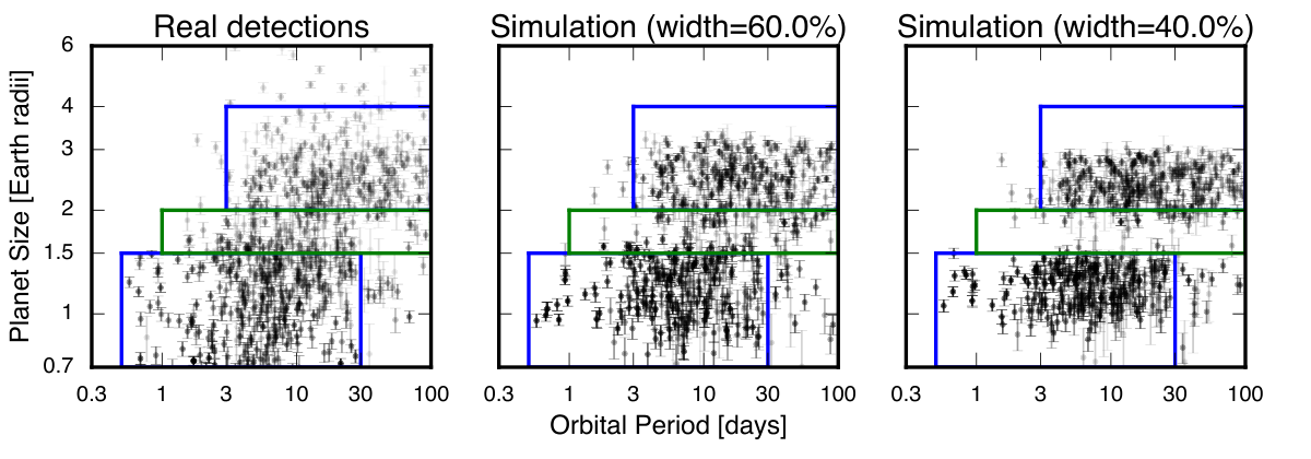
We show the filtered distribution of planets in Figure 7, and we identify two fiducial planet classes, “super-Earths” and “sub-Neptunes,” as well as the radius gap. The large number of planets (129) residing within the gap appear to be inconsistent with scatter from above and below. To test this, we constructed a toy model to assess whether they could be explained by measurement uncertainties alone.
In or toy model, we took the observed planet detections and assigned them to one of the two planet classes, based on whether they resided in one of the two boxes shown in Figure 7. For each super-Earth and sub-Neptune we assigned a new radius from uniform distributions with centers at 1.2 or 2.4 , respectively, which correspond to the locations of the observed peaks in the radius distribution. The orbital periods were retained from the actual detections. The fractional width shared by both distributions is a free parameter in this model.
We simulated planet detections over a range of and computed a figure of merit , where is the number of detections within box (plotted in Figure 7).
The FOM and visual inspection identified an intrinsic spread of as a good match to the data (see Figure 7). In our best-fitting toy model, the super-Earth and sub-Neptune populations span 0.85 to 1.55 and 1.7 to 3.1 , respectively; it is inconsistent with a population devoid of planets between 1.5 and 2.0 .
As a limiting case, we show a model with in Figure 7. Here, the super-Earth and sub-Neptune population span 0.96 to 1.44 and 1.92 to 2.88 , respectively, which approximate the upper and lower boundaries of the gap. This model produces a much emptier gap and is an obvious mismatch with the observations.
We recognize that this toy model does not capture the detailed radius distribution of planets, most notably the tail of planets larger than 3 . A more detailed study might use a different distribution to model the planet radii, such as a Gaussian, Rayleigh, or a non-parametric distribution. Nonetheless, we have constrained the intrinsic dispersion in the size of the super-Earth and sub-Neptune populations to be 60%. While there is a dip in the occurrence of close-in planets from 1.5 to 2.0 , occurrence does not fall to zero. These interpretations were not possible in previous studies, due to larger radius uncertainties or limited numbers of detected planets.
IV.4 Trends with Host-Star Mass
We plot planet size vs. stellar mass in Figure 8 in order to investigate potential changes in the structure of the planet radius distribution as a function of stellar host mass. This Figure shows that the transition radius between the two populations increases monotonically with stellar mass. The gap occurs near 1.6 for planets orbiting host stars with masses near 0.8 and moves to 2.0 for planets orbiting stars with masses above 1.2 . We also split the sample into three bins of stellar mass: 0.96 , = 0.96–1.11 , and 1.11 . We chose bin boundaries such that the three bins captured equal numbers of planets. Figure 9 shows the planet population in the - and - planes for each of the three mass bins. The gap is clearly visible in each of the three stellar mass bins, and appears wider than the gap from the combined sample shown in Figure 6.
We observe several trends with stellar mass. First, the typical size of super-Earth and sub-Neptune planets increases with increasing stellar mass, an observation that we quantify later in this section. This explains why the planet populations are better separated when one considers a narrow range of stellar mass; when all three mass groups are combined the distributions overlap. It also helps to clarify why the planet populations in Van Eylen et al. (2017) seemed to be more separated compared to those in F17. The asteroseismic sample was heavily weighted toward stars more massive than the sun, and is more directly comparable to the – distribution of our high mass bin. The top right panel of our Figure 9 is a closer match to Figure 2 from Van Eylen et al. (2017) than the upper left panel of our Figure 9.
To quantify the change in typical planet size with stellar mass, we calculated the mean planet radius for sub-Neptunes (1.7–4.0 , and days) and super-Earths (1.0–1.7 , and days). We weighted each radius by the weights used in the occurrence calculations, described in Section IV.2. Figure 10 shows these mean planet parameters as a function of stellar mass. Consistent with visual inspection of Figure 9, we see monotonically increasing planet size with increasing stellar host star mass in both the super-Earth and sub-Neptune planets.
Although the trend with stellar mass is strong, we caution that stellar metallicity may be a confounding factor. More massive stars are younger on average and are thus more metal-rich due to galactic chemical enrichment. Indeed, Petigura et al. (2018) observed a correlation between planet size and host star metallicity in the CKS sample and this correlation has been observed previously in many different samples (Santos et al. 2004; Fischer & Valenti 2005; Sousa et al. 2008; Ghezzi et al. 2010; Buchhave et al. 2014; Schlaufman 2015; Wang & Fischer 2015, e.g.). The solid component of the protoplanetary disk likely tracks both stellar metallicity and stellar mass. Therefore, we expect planet size to be correlated with both stellar mass and metallicity. Future studies spanning a larger range of stellar mass and metallicity are necessary to resolve this ambiguity.
Previous studies have noted a desert of highly-irradiated sub-Neptune planets (see, e.g., Lundkvist et al. 2016 and Mazeh et al. 2016). We observe this sub-Neptune desert in our three mass bins (Figure 9), but note that it shifts to higher incident stellar flux around high mass stars. This trend is highly significant. Figure 10 shows the average as function . The mean for both the super-Earths and sub-Neptunes increases by over a relatively narrow range of average , 0.85 to 1.2 . One explanation could be that the orbital periods of small planets decreases with stellar mass. However, the mean orbital periods for the three different mass bins are consistent to 30%.
Figure 11 shows the cumulative fraction of hot ( = 30–3000 ) sub-Neptune size planets ( = 1.7–4.0 ) as a function of insolation flux, highlighting the shift of the sub-Neptune desert with stellar mass. In the high stellar mass sample, 10% of planets have 300 . For the low stellar mass sample, one must include planets out to 150 to encompass 10% of the population.


V Discussion and Conclusions
We analyzed the Kepler planet population after improving the radius precision of the stellar hosts and their planets. This improvement leveraged both CKS spectroscopy and Gaia DR2 parallaxes. Our median stellar radius precision is now 2% compared to 11% in J17. The uncertainty in our planet radii are now typically 5% and are limited by uncertainties in the Kepler transit modeling, rather than the stellar radius uncertainties as in J17.
With these improved planet radii, we examined the population of small planets at higher resolution. We confirmed the existence of the F17 radius gap between 1.5 and 2.0 , with more precise and independently derived planet radii. The overall radius distribution is similar to that of F17, which demonstrates that we are resolving the intrinsic spread of the super-Earth and sub-Neptune populations, which span 60% in radius. We also demonstrated that the gap from 1.5 to 2.0 is not devoid of planets, a conclusion previously obscured by measurement uncertainties or small sample sizes. We observed a correlation of the average planet size and average insolation flux with stellar host mass. However, there is no significant correlation in the average orbital period as a function of average stellar host mass.
Here, we interpret our findings in the context of two theories that have been proposed to explain the distribution planets between the size of Earth and Neptune:
- 1.
Mass loss by photoevaporation. In this mechanism, X-ray and UV radiation heats the outer layers of a planet’s envelope and drives mass loss. Several groups considered photoevaporation and predicted the planet radius gap before it was observed in F17, including Owen & Wu (2013), Lopez & Fortney (2013), Jin et al. (2014), and Chen & Rogers (2016). Following F17, Owen & Wu (2017) developed additional analytic photoevaporation theory and performed a population synthesis analysis comparing their simulated populations to the F17 occurrence measurements.
- 2.
Core-powered mass loss. In this mechanism, luminosity from a cooling rocky core heats a planet’s envelope and drives mass loss. Ginzburg et al. (2016) developed the theory of core-powered mass loss and computed mass loss rates. Ginzburg et al. (2018) performed a population synthesis with comparisons to the F17 radius distribution and demonstrated that core-powered mass loss could explain the bimodal radius distribution.
Both theories can explain a bimodal population of planet sizes composed of two subpopulations: a population of bare rocky cores and a population with H/He envelopes with mass fractions of a few percent. Because both mass loss mechanisms are more efficient at high levels of incident stellar flux, they both predict that the population of sub-Neptunes should be offset to lower insolation fluxes compared to the super-Earths
A key difference between the two mechanisms is the expected dependence on stellar mass. Core-powered mass loss depends only on properties of the planet and bolometric incident stellar flux. All else being equal, this mechanism predicts no dependence of the planet population as a function of . In contrast, the efficiency of photoevaporation depends on the time-integrated XUV flux, or “fluence.” This quantity is a strong function of stellar mass since (Jackson et al. 2012). Therefore, photoevaporation predicts that the population of sub-Neptunes should shift to lower with decreasing stellar mass, due to increased activity around lower mass stars. The shifts in the - distribution of planets with are consistent with this prediction from photoevaporation.
The lack of a strong – dependence is also consistent with photoevaporation. Owen & Wu (2017) showed that the mass loss timescale . Photoevaporation thus has a steeper dependence on at fixed than at fixed . This naturally explains why we see a strong trend in planet with stellar mass and no significant trend with in Figure 10.
Other super-Earth formation mechanisms have been proposed that could potentially produce a gap in the size distribution including delayed formation in a gas-poor disk (Lee et al. 2014; Lee & Chiang 2016, e.g.), and sculpting by giant impacts (Liu et al. 2015; Schlichting et al. 2015; Inamdar & Schlichting 2016, e.g.). Formation in a gas-poor disk without any sculpting by photoevaporation would produce a gap radius that does not change with orbital period and is inconsistent with the results of Van Eylen et al. (2017). Sculpting by giant impacts alone predicts that the gap radius would be found at larger radii at longer orbital periods (Lopez & Rice 2016) which is the opposite of the trend found by Van Eylen et al. (2017).
We interpret the observed stellar mass dependence of the planet population as evidence supporting photoevaporation model. However, these mechanisms are not mutually exclusive and all of them could be operating simultaneously or or at different times during the formation of planetary systems. If photoevaporation is the dominate mechanism for sculpting planet envelopes, one may fit the observed distribution of planets to constrain important quantities like the distribution of planet core masses, envelope fractions, and core compositions (Owen & Wu 2017).
Due to the magnitude-limited nature of CKS, our analysis was restricted to a fairly narrow range in , spanning 0.85 to 1.2 . Previous studies of the radius distribution of planets orbiting M dwarfs have shown that these planets tend to be smaller on average (Morton & Swift 2014; Dressing & Charbonneau 2015). This may be an extension of the stellar mass dependence of the planet population observed in this work. However, no study of planets orbiting low-mass stars to date has detected a gap in the radius distribution. Such a detection (or lack thereof) would reveal insights into the structure and formation of planets around low-mass stars. This motivates future high precision studies of large samples of planets orbiting K and M dwarfs. Such studies would provide additional leverage on to test the dependence of the planet population on stellar mass and to constrain the mechanisms that form and sculpt planets.
Keck:I (HIRES), Kepler, Gaia
References
- Arenou et al. (2018) Arenou, F., Luri, X., Babusiaux, C., et al. 2018, ArXiv e-prints, arXiv:1804.09375
- Astraatmadja & Bailer-Jones (2016) Astraatmadja, T. L., & Bailer-Jones, C. A. L. 2016, ApJ, 833, 119
- Astropy Collaboration et al. (2013) Astropy Collaboration, Robitaille, T. P., Tollerud, E. J., et al. 2013, A&A, 558, A33
- Borucki (2016) Borucki, W. J. 2016, Reports on Progress in Physics, 79, 036901
- Borucki et al. (2010) Borucki, W. J., Koch, D., Basri, G., et al. 2010, Science, 327, 977
- Brewer et al. (2016) Brewer, J. M., Fischer, D. A., Valenti, J. A., & Piskunov, N. 2016, ApJS, 225, 32
- Brown et al. (2011) Brown, T. M., Latham, D. W., Everett, M. E., & Esquerdo, G. A. 2011, AJ, 142, 112
- Buchhave et al. (2014) Buchhave, L. A., Bizzarro, M., Latham, D. W., et al. 2014, Nature, 509, 593
- Casagrande & VandenBerg (2014) Casagrande, L., & VandenBerg, D. A. 2014, MNRAS, 444, 392
- Chen & Rogers (2016) Chen, H., & Rogers, L. A. 2016, ApJ, 831, 180
- Choi et al. (2016) Choi, J., Dotter, A., Conroy, C., et al. 2016, ApJ, 823, 102
- Christiansen et al. (2015) Christiansen, J. L., Clarke, B. D., Burke, C. J., et al. 2015, ApJ, 810, 95
- Dressing & Charbonneau (2015) Dressing, C. D., & Charbonneau, D. 2015, ApJ, 807, 45
- Fischer & Valenti (2005) Fischer, D. A., & Valenti, J. 2005, ApJ, 622, 1102
- Fressin et al. (2013) Fressin, F., Torres, G., Charbonneau, D., et al. 2013, ApJ, 766, 81
- Fulton et al. (2017) Fulton, B. J., Petigura, E. A., Howard, A. W., et al. 2017, AJ, 154, 109
- Furlan et al. (2017) Furlan, E., Ciardi, D. R., Everett, M. E., et al. 2017, The Astronomical Journal, 153, 71
- Gaia Collaboration et al. (2018) Gaia Collaboration, Brown, A. G. A., Vallenari, A., et al. 2018, ArXiv e-prints, arXiv:1804.09365
- Gaia Collaboration et al. (2016a) Gaia Collaboration, Prusti, T., de Bruijne, J. H. J., et al. 2016a, A&A, 595, A1
- Gaia Collaboration et al. (2016b) Gaia Collaboration, Brown, A. G. A., Vallenari, A., et al. 2016b, A&A, 595, A2
- Ghezzi et al. (2010) Ghezzi, L., Cunha, K., Smith, V. V., et al. 2010, ApJ, 720, 1290
- Ginzburg et al. (2016) Ginzburg, S., Schlichting, H. E., & Sari, R. 2016, ApJ, 825, 29
- Ginzburg et al. (2018) —. 2018, MNRAS, 476, 759
- Green et al. (2018) Green, G. M., Schlafly, E. F., Finkbeiner, D., et al. 2018, ArXiv e-prints, arXiv:1801.03555
- Holman et al. (2010) Holman, M. J., Fabrycky, D. C., Ragozzine, D., et al. 2010, Science, 330, 51
- Howard et al. (2010) Howard, A. W., Marcy, G. W., Johnson, J. A., et al. 2010, Science, 330, 653
- Howard et al. (2012) Howard, A. W., Marcy, G. W., Bryson, S. T., et al. 2012, ApJS, 201, 15
- Hsu et al. (2018) Hsu, D. C., Ford, E. B., Ragozzine, D., & Morehead, R. C. 2018, AJ, 155, 205
- Huber et al. (2013) Huber, D., Chaplin, W. J., Christensen-Dalsgaard, J., et al. 2013, ApJ, 767, 127
- Huber et al. (2014) Huber, D., Silva Aguirre, V., Matthews, J. M., et al. 2014, ApJS, 211, 2
- Huber et al. (2017) Huber, D., Zinn, J., Bojsen-Hansen, M., et al. 2017, ApJ, 844, 102
- Hunter (2007) Hunter, J. D. 2007, Computing In Science & Engineering, 9, 90
- Inamdar & Schlichting (2016) Inamdar, N. K., & Schlichting, H. E. 2016, ApJ, 817, L13
- Indebetouw et al. (2005) Indebetouw, R., Mathis, J. S., Babler, B. L., et al. 2005, ApJ, 619, 931
- Jackson et al. (2012) Jackson, A. P., Davis, T. A., & Wheatley, P. J. 2012, MNRAS, 422, 2024
- Jin et al. (2014) Jin, S., Mordasini, C., Parmentier, V., et al. 2014, ApJ, 795, 65
- Johnson et al. (2017) Johnson, J. A., Petigura, E. A., Fulton, B. J., et al. 2017, ArXiv e-prints, arXiv:1703.10402
- Lee & Chiang (2016) Lee, E. J., & Chiang, E. 2016, ApJ, 817, 90
- Lee et al. (2014) Lee, E. J., Chiang, E., & Ormel, C. W. 2014, ApJ, 797, 95
- Lindegren et al. (2016) Lindegren, L., Lammers, U., Bastian, U., et al. 2016, A&A, 595, A4
- Liu et al. (2015) Liu, S.-F., Hori, Y., Lin, D. N. C., & Asphaug, E. 2015, ApJ, 812, 164
- Lopez & Fortney (2013) Lopez, E. D., & Fortney, J. J. 2013, The Astrophysical Journal, 776, 2
- Lopez & Rice (2016) Lopez, E. D., & Rice, K. 2016, ArXiv e-prints, arXiv:1610.09390
- Lundkvist et al. (2016) Lundkvist, M. S., Kjeldsen, H., Albrecht, S., et al. 2016, Nature Communications, 7, 11201
- Mamajek et al. (2015) Mamajek, E. E., Torres, G., Prsa, A., et al. 2015, ArXiv e-prints, arXiv:1510.06262
- Marcy et al. (2014) Marcy, G. W., Isaacson, H., Howard, A. W., et al. 2014, ApJS, 210, 20
- Mathur et al. (2017) Mathur, S., Huber, D., Batalha, N. M., et al. 2017, ApJS, 229, 30
- Mazeh et al. (2016) Mazeh, T., Holczer, T., & Faigler, S. 2016, A&A, 589, A75
- McKinney (2010) McKinney, W. 2010, in Proceedings of the 9th Python in Science Conference, ed. S. van der Walt & J. Millman, 51 – 56
- Morton & Swift (2014) Morton, T. D., & Swift, J. 2014, ApJ, 791, 10
- Mullally et al. (2015) Mullally, F., Coughlin, J. L., Thompson, S. E., et al. 2015, ApJS, 217, 31
- Newville et al. (2014) Newville, M., Stensitzki, T., Allen, D. B., & Ingargiola, A. 2014, LMFIT: Non-Linear Least-Square Minimization and Curve-Fitting for Python, , , doi:10.5281/zenodo.11813. https://doi.org/10.5281/zenodo.11813
- Nishiyama et al. (2008) Nishiyama, S., Nagata, T., Tamura, M., et al. 2008, ApJ, 680, 1174
- Owen & Wu (2013) Owen, J. E., & Wu, Y. 2013, ApJ, 775, 105
- Owen & Wu (2017) —. 2017, ApJ, 847, 29
- Petigura et al. (2013) Petigura, E. A., Howard, A. W., & Marcy, G. W. 2013, Proceedings of the National Academy of Science, 110, 19273
- Petigura et al. (2017) Petigura, E. A., Howard, A. W., Marcy, G. W., et al. 2017, AJ, 154, 107
- Petigura et al. (2018) Petigura, E. A., Marcy, G. W., Winn, J. N., et al. 2018, AJ, 155, 89
- Pinsonneault et al. (2012) Pinsonneault, M. H., An, D., Molenda-Żakowicz, J., et al. 2012, ApJS, 199, 30
- Rogers (2015) Rogers, L. A. 2015, ApJ, 801, 41
- Santos et al. (2004) Santos, N. C., Israelian, G., & Mayor, M. 2004, A&A, 415, 1153
- Schlafly et al. (2016) Schlafly, E. F., Meisner, A. M., Stutz, A. M., et al. 2016, ApJ, 821, 78
- Schlaufman (2015) Schlaufman, K. C. 2015, ApJ, 799, L26
- Schlichting et al. (2015) Schlichting, H. E., Sari, R., & Yalinewich, A. 2015, Icarus, 247, 81
- Silva Aguirre et al. (2015) Silva Aguirre, V., Davies, G. R., Basu, S., et al. 2015, MNRAS, 452, 2127
- Skrutskie et al. (2006) Skrutskie, M. F., Cutri, R. M., Stiening, R., et al. 2006, AJ, 131, 1163
- Sousa et al. (2008) Sousa, S. G., Santos, N. C., Mayor, M., et al. 2008, A&A, 487, 373
- van der Walt et al. (2011) van der Walt, S., Colbert, S. C., & Varoquaux, G. 2011, Computing in Science Engineering, 13, 22
- Van Eylen et al. (2017) Van Eylen, V., Agentoft, C., Lundkvist, M. S., et al. 2017, ArXiv e-prints, arXiv:1710.05398
- Wang & Fischer (2015) Wang, J., & Fischer, D. A. 2015, AJ, 149, 14
- Weiss & Marcy (2014) Weiss, L. M., & Marcy, G. W. 2014, ApJ, 783, L6
- Zinn et al. (2018) Zinn, J. C., Pinsonneault, M. H., Huber, D., & Stello, D. 2018, ArXiv e-prints, arXiv:1805.02650
| KOI | [Fe/H] | ageiso | RCF | |||||||||
|---|---|---|---|---|---|---|---|---|---|---|---|---|
| K | dex | mag | mas | g/cc | dex | mas | ||||||
| K00001 | 5819 | 0.01 | 9.8 | 4.67 | 1.04 | 0.99 | 1.04 | 0.87 | 9.74 | 4.76 | 1.00 | 1.010 |
| K00002 | 6449 | 0.20 | 9.3 | 2.96 | 1.97 | 1.51 | 1.96 | 0.20 | 9.25 | 3.66 | 1.00 | 1.003 |
| K00006 | 6348 | 0.04 | 11.0 | 2.13 | 1.30 | 1.20 | 1.28 | 0.57 | 9.32 | 2.20 | 1.01 | 1.001 |
| K00007 | 5827 | 0.18 | 10.8 | 2.07 | 1.51 | 1.15 | 1.51 | 0.34 | 9.78 | 2.11 | 1.00 | |
| K00008 | 5891 | -0.07 | 11.0 | 3.01 | 0.94 | 1.00 | 0.93 | 1.23 | 9.18 | 2.90 | 1.00 | |
| K00010 | 6181 | -0.08 | 12.3 | 1.00 | 1.54 | 1.15 | 1.53 | 0.32 | 9.67 | 1.21 | 1.01 | 1.001 |
| K00017 | 5660 | 0.36 | 11.6 | 1.73 | 1.26 | 1.09 | 1.25 | 0.56 | 9.81 | 1.54 | 1.03 | |
| K00018 | 6332 | 0.02 | 11.8 | 1.14 | 1.74 | 1.31 | 1.69 | 0.27 | 9.46 | 1.25 | 1.02 | 1.005 |
| K00020 | 5926 | 0.03 | 12.1 | 1.16 | 1.50 | 1.09 | 1.50 | 0.32 | 9.83 | 1.10 | 1.00 | |
| K00022 | 5891 | 0.21 | 12.0 | 1.41 | 1.25 | 1.12 | 1.25 | 0.58 | 9.67 | 1.31 | 1.00 | |
| K00041 | 5854 | 0.10 | 9.8 | 3.31 | 1.53 | 1.10 | 1.52 | 0.31 | 9.84 | 3.41 | 1.00 | 1.008 |
| K00046 | 5661 | 0.39 | 12.0 | 1.10 | 1.66 | 1.24 | 1.64 | 0.28 | 9.72 | 1.19 | 1.00 |
Note. — Properties of planet hosting stars. and [Fe/H] are from P17, is the -band apparent magnitude from 2MASS (Skrutskie et al. 2006, see Section III.2), is the trigonometric parallax from Gaia DR2 (Gaia Collaboration et al. 2018, see Section III.4). The following quantities are described in Section III.7: is the adopted stellar radius, computed using the Stefan-Boltzmann law; stellar properties with the ‘iso’ subscript incorporate constraints from the MIST isochrones; and is the “spectroscopic parallax.” encodes contaminating flux from neighboring stars within 8 arcsec in -band (see Section IV.2). RCF is the “radius correction factor” computed by Furlan et al. (2017) (see Section IV.2). Table 2 is published in its entirety in machine-readable format. A portion is shown here for guidance regarding its form and content.
| Planet | / | |||||
|---|---|---|---|---|---|---|
| candidate | d | AU | ||||
| K00001.01 | 2.5 | 0.124 | 14.14 | 0.036 | 882 | |
| K00002.01 | 2.2 | 0.075 | 16.25 | 0.038 | 4161 | |
| K00006.01 | 1.3 | 0.294 | 41.94 | 0.025 | 3852 | |
| K00007.01 | 3.2 | 0.025 | 4.08 | 0.045 | 1180 | |
| K00008.01 | 1.2 | 0.019 | 1.90 | 0.022 | 2031 | |
| K00010.01 | 3.5 | 0.094 | 15.70 | 0.047 | 1375 | |
| K00017.01 | 3.2 | 0.095 | 13.10 | 0.044 | 753 | |
| K00018.01 | 3.5 | 0.080 | 15.23 | 0.050 | 1759 | |
| K00020.01 | 4.4 | 0.118 | 19.38 | 0.054 | 848 | |
| K00022.01 | 7.9 | 0.094 | 12.85 | 0.081 | 260 | |
| K00041.01 | 12.8 | 0.014 | 2.34 | 0.111 | 201 | |
| K00041.02 | 6.9 | 0.008 | 1.34 | 0.073 | 459 | |
| K00041.03 | 35.3 | 0.009 | 1.54 | 0.217 | 52 | |
| K00046.01 | 3.5 | 0.033 | 5.97 | 0.048 | 1076 | |
| K00046.02 | 6.0 | 0.007 | 1.24 | 0.070 | 520 |
Note. — Planetary properties. Period and planet-to-star radius ratio are from Mullally et al. (2015). Planet size , semi-major axis , and incident stellar flux relative to Earth are derived from the updated stellar properties in Table 2. Table 2 is published in its entirety in machine-readable format with full numerical precision and uncertainties. A portion is shown here for guidance regarding its form and content.
| Planet | SNR | Detection probability | Transit probability | Weight |
|---|---|---|---|---|
| candidate | ||||
| K00958.01 | 186.24 | 0.97 | 0.02 | 49.24 |
| K04053.01 | 21.03 | 0.77 | 0.17 | 7.71 |
| K04212.02 | 8.77 | 0.81 | 0.05 | 22.85 |
| K04212.01 | 16.53 | 0.93 | 0.08 | 13.79 |
| K01001.01 | 37.27 | 0.99 | 0.03 | 32.14 |
| K01001.02 | 15.49 | 0.96 | 0.01 | 75.81 |
| K02534.01 | 22.64 | 0.94 | 0.11 | 9.37 |
| K02534.02 | 11.91 | 0.84 | 0.08 | 15.49 |
| K02403.01 | 17.98 | 0.79 | 0.04 | 29.89 |
| K00988.01 | 60.03 | 0.97 | 0.04 | 28.79 |