跳到论文正文
W Papers独立论文阅读器 arXiv:1805.00897 论文正文 计算阅读时间 · 0%
引用这篇论文根据当前论文元数据生成,正式投稿前建议核对。


License: arXiv.org perpetual non-exclusive license
arXiv:1805.00897v2 [math.OC] 13 Nov 2018

On the Design of Hybrid Pose and Velocity-bias Observers on Lie Group S​E​(3)SE(3)

Miaomiao Wang and Abdelhamid Tayebi ††thanks: This work was supported by the National Sciences and Engineering Research Council of Canada (NSERC). A preliminary and partial version of this work was presented in [1].††thanks: The authors are with the Department of Electrical and Computer Engineering, University of Western Ontario, London, Ontario, Canada. A. Tayebi is also with the Department of Electrical Engineering, Lakehead University, Thunder Bay, Ontario, Canada. mwang448@uwo.ca, atayebi@lakeheadu.ca
Abstract

This paper deals with the design of globally exponentially stable invariant observers on the Special Euclidian group S​E​(3)SE(3). First, we propose a generic hybrid observer scheme (depending on a generic potential function) evolving on S​E​(3)×ℝ6SE(3)\times\mathbb{R}^{6} for pose (orientation and position) and velocity-bias estimation. Thereafter, the proposed observer is formulated explicitly in terms of inertial vectors and landmark measurements. Interestingly, the proposed observer leads to a decoupled rotational error dynamics from the translational dynamics, which is an interesting feature in practical applications with noisy measurements and disturbances.

Index terms—Nonlinear Observer, Special Euclidean group S​E​(3)SE(3), Hybrid dynamics, Inertial-vision systems.

1 Introduction

The development of reliable pose (i.e, attitude and position) estimation algorithms is instrumental in many applications such as autonomous underwater vehicles and unmanned aerial vehicles. Since there is no sensor that directly measures the attitude, the latter is usually determined using body-frame measurements of some known inertial vectors via static determination algorithms [2] which are generally sensitive to measurement noise. Alternatively, dynamic estimation algorithms using inertial vector measurements together with the angular velocity can be used to recover the attitude while filtering measurement noise (e.g., Kalman filters [3], linear complementary filters [4], nonlinear complementary filters [5]). In low-cost applications, angular velocity and inertial vector measurements can be obtained, for instance, from an inertial measurement unit (IMU) equipped with gyroscopes, accelerometers and magnetometers. The translational position and velocity can be estimated using a Global Positioning System (GPS). However, in GPS-denied environments such as indoor applications, recovering the position and linear velocity is a challenging task. Alternatively, inertial-vision systems combining IMU and on-board camera measurements have been considered for pose estimation [6, 7, 8]. In [7], local Riccati-based pose observers have been proposed relying on the system’s linear and angular velocities and the bearing measurements of some known landmark points. Another solution with global asymptotic stability (GAS) has been proposed in[8], which considers a non-geometric pose estimation problem using biased body-frame measurements of the system’s linear and angular velocities as well as body-frame measurements of landmarks. The achieved global asymptotic stability results are due to the fact that the estimates are not confined to live in S​E​(3)SE(3) for all times.

Recently, a class of nonlinear observers on Lie groups including S​O​(3)SO(3) and S​E​(3)SE(3) have made their appearances in the literature. Invariant observers which take into account the topological properties of the motion space were developed in [5, 9, 10]. Motivated by the work of [5] on S​O​(3)SO(3), complementary observers on S​E​(3)SE(3) were proposed in [11, 12]. In practice, measurements of group velocity (translational and rotational velocities) are often corrupted by an unknown bias. Pose estimation using biased velocity measurements were considered in [13, 14, 15]. A nice feature of [15] is the fact that the observer incorporates (naturally) both inertial vector measurements (e.g., from IMU) and landmark measurements (e.g., from a vision system). The observers proposed in [11, 12, 13, 14, 15] are shown to guarantee almost global asymptotic stability (AGAS), i.e., the estimated pose converges to the actual one from almost all initial conditions except from a set of Lebesgue measure zero. This is the strongest result one can aim at when considering continuous time-invariant state observers on S​O​(3)SO(3) or S​E​(3)SE(3).

Recently, the topological obstruction to global asymptotic stability on S​O​(3)SO(3) using continuous time-invariant controllers (observers) has been successfully addressed via hybrid techniques such as [16, 17, 18, 19, 20]. To this end, a synergistic hybrid technique was introduced in [16]. Motivated by this approach, globally asymptotically stable hybrid attitude observers on S​O​(3)SO(3) have been proposed in [17] and globally exponentially stable hybrid attitude observers on S​O​(3)SO(3) have been proposed in [20].

In this paper we propose an generic approach for hybrid observers design on S​E​(3)SE(3) leading to global exponential stability. To the best of our knowledge, there is no work in the literature achieving such results on S​E​(3)SE(3). Moreover, we propose some explicit and practically implementable versions of the proposed scheme, using biased group-velocity measurements (constant bias), inertial vectors and landmark measurements. Interestingly, the proposed observer leads to a decoupled rotational error dynamics from the translational error dynamics, which guarantees nice robustness and performance properties.

The remainder of this paper is organized as follows. Section 2 introduces some preliminary notions that will be used throughout out the paper. In Section 3, the problem of pose estimation on S​E​(3)SE(3) is formulated. In Section 4, a hybrid approach for pose and velocity-bias estimation is proposed. An estimation scheme leading to decoupled rotational error dynamics from the translational error dynamics is provided in Section 5. Section 6 presents some simulation results showing the performance of the proposed estimation schemes.

2 Background and Preliminaries

2.1 Notations and mathematical preliminaries

The sets of real, nonnegative real and natural number are denoted as ℝ\mathbb{R}, ℝ≥0\mathbb{R}_{\geq 0} and ℕ\mathbb{N}, respectively. We denote by ℝn\mathbb{R}^{n} the nn-dimensional Euclidean space and 𝕊n\mathbb{S}^{n} the set of nn-dimensional unit vectors. Given two matrices, A,B∈ℝm×nA,B\in\mathbb{R}^{m\times n}, their Euclidean inner product is defined as ⟨⟨A,B⟩⟩:=tr⁡(A⊤​B)\langle\langle A,B\rangle\rangle:=\mathrm{tr}(A^{\top}B). The Euclidean norm of a vector x∈ℝnx\in\mathbb{R}^{n} is defined as ‖x‖:=x⊤​x\|x\|:=\sqrt{x^{\top}x}, and the Frobenius norm of a matrix X∈ℝn×mX\in\mathbb{R}^{n\times m} is given by ‖X‖F:=⟨⟨X,X⟩⟩\|X\|_{F}:=\sqrt{\langle\langle X,X\rangle\rangle}. The nn-by-nn identity matrix is denoted by InI_{n}. For a matrix A∈ℝn×nA\in\mathbb{R}^{n\times n}, we define ℰ⁡(A)\mathcal{E}(A) as the set of all eigenvectors of AA and 𝔼⁡(A)⊆ℰ⁡(A)\mathbb{E}(A)\subseteq\mathcal{E}(A) as the eigenbasis set of AA. Let λiA\lambda^{A}_{i} be the ii-th eigenvalue of AA, and λminA\lambda^{A}_{\min} and λmaxA\lambda^{A}_{\max} be the minimum and maximum eigenvalue of AA, respectively.

Let SO(3):={R∈ℝ3×3|R⊤R=I3,det(R)=1}SO(3):=\{R\in\mathbb{R}^{3\times 3}|R^{\top}R=I_{3},\det(R)=1\} be the 3-dimensional Special Orthogonal group S​O​(3)SO(3). Consider the 33-dimensional Special Euclidean group, defined as

SE(3):={g=𝒯(R,p)∈ℝ4×4|R∈SO(3),p∈ℝ3},SE(3):=\left\{g=\mathcal{T}(R,p)\in\mathbb{R}^{4\times 4}\left|R\in SO(3),p\in\mathbb{R}^{3}\right.\right\},

with the map 𝒯:S​O​(3)×ℝ3→S​E​(3)\mathcal{T}:SO(3)\times\mathbb{R}^{3}\to SE(3) given by

𝒯⁡(R,p):=[Rp01].\mathcal{T}(R,p):=\begin{bmatrix}R&p\\ 0&1\end{bmatrix}.

On any Lie group the tangent space at the group identity has the structure of a Lie algebra. Let 𝔰​𝔬​(3):={Ω∈ℝ3×3|Ω⊤=−Ω}\mathfrak{so}(3):=\{\Omega\in\mathbb{R}^{3\times 3}|\Omega^{\top}=-\Omega\} be the Lie algebra of S​O​(3)SO(3). The Lie algebra of S​E​(3)SE(3), denoted by 𝔰​𝔢​(3)\mathfrak{se}(3), is given by

𝔰​𝔢​(3)\displaystyle\mathfrak{se}(3) :={X∈ℝ4×4|X=[Ωv00],Ω∈𝔰𝔬(3),v∈ℝ3}.\displaystyle:=\left\{X\in\mathbb{R}^{4\times 4}|X=\begin{bmatrix}\Omega&v\\ 0&0\end{bmatrix},\Omega\in\mathfrak{so}(3),v\in\mathbb{R}^{3}\right\}.

Let ×\times be the vector cross-product on ℝ3\mathbb{R}^{3} and define the map (⋅)×:ℝ3↦𝔰​𝔬​(3)(\cdot)^{\times}:\mathbb{R}^{3}\mapsto\mathfrak{so}(3) such that x×y=x×​yx\times y=x^{\times}y, for any x,y∈ℝ3x,y\in\mathbb{R}^{3}. A wedge map (⋅)∧:ℝ6↦𝔰​𝔢​(3)(\cdot)^{\wedge}:\mathbb{R}^{6}\mapsto\mathfrak{se}(3) is defined as

ξ∧:=[ω×v00],ξ:=[ωv].\xi^{\wedge}:=\begin{bmatrix}\omega^{\times}&v\\ 0&0\end{bmatrix},\hskip 9.24994pt\xi:=\begin{bmatrix}\omega\\ v\end{bmatrix}.

The tangent space of the group S​E​(3)SE(3), is identified by TgSE(3):={gX|g∈SE(3),X∈𝔰𝔢(3)}.T_{g}SE(3):=\{gX|\ g\in SE(3),X\in\mathfrak{se}(3)\}. Let ⟨⋅,⋅⟩g:Tg​S​E​(3)×Tg​S​E​(3)→ℝ\langle\cdot,\cdot\rangle_{g}:T_{g}SE(3)\times T_{g}SE(3)\to\mathbb{R} be a Riemannian metric on S​E​(3)SE(3), such that

⟨gX,gY⟩g:=⟨⟨X,Y⟩⟩,g∈SE(3),X,Y∈𝔰𝔢(3).\displaystyle\langle gX,gY\rangle_{g}:=\langle\langle X,Y\rangle\rangle,\hskip 9.24994ptg\in SE(3),X,Y\in\mathfrak{se}(3).

Given a differentiable smooth function f:S​E​(3)→ℝf:SE(3)\to\mathbb{R}, the gradient of ff , denoted ∇gf∈Tg​S​E​(3)\nabla_{g}f\in T_{g}SE(3), relative to the Riemannian metric ⟨⋅,⋅⟩g\langle\cdot,\cdot\rangle_{g} is uniquely defined by

d​f⋅g​X=⟨∇gf,g​X⟩g=⟨⟨g−1​∇gf,X⟩⟩,df\cdot gX=\langle\nabla_{g}f,gX\rangle_{g}=\langle\langle g^{-1}\nabla_{g}f,X\rangle\rangle,

For all g∈S​E​(3),X∈𝔰​𝔢​(3)g\in SE(3),X\in\mathfrak{se}(3). A point g∈S​E​(3)g\in SE(3) is called critical point of ff if the gradient of ff at gg is zero (i.e., ∇gf=0\nabla_{g}f=0). The set of all critical points of ff on S​E​(3)SE(3) is denoted by 𝒞​f:={g∈S​E​(3)|∇gf=0}⊆S​E​(3)\mathcal{C}f:=\{g\in SE(3)|\nabla_{g}f=0\}\subseteq SE(3). For any g∈S​E​(3)g\in SE(3), we define |g|I|g|_{I} as the distance with respect to I4I_{4}, which is given by |g|I:=‖I4−g‖F|g|_{I}:=\|I_{4}-g\|_{F}. The map ℛa:ℝ×𝕊2→S​O​(3)\mathcal{R}_{a}:\mathbb{R}\times\mathbb{S}^{2}\to SO(3) known as the angle-axis parametrization of S​O​(3)SO(3) is defined as ℛa​(θ,u):=I3+sin⁡θ​u×+(1−cos⁡θ)​(u×)2.\mathcal{R}_{a}(\theta,u):=I_{3}+\sin\theta u^{\times}+(1-\cos\theta)(u^{\times})^{2}.

For a matrix A∈ℝ3×3A\in\mathbb{R}^{3\times 3}, we denote by ℙa​(A)\mathbb{P}_{a}(A) as the anti-symmetric projection of A, such that ℙa​(A)=(A−A⊤)/2\mathbb{P}_{a}(A)=(A-A^{\top})/2. Let ℙ:ℝ4×4→𝔰​𝔢​(3)\mathbb{P}:\mathbb{R}^{4\times 4}\rightarrow\mathfrak{se}(3) denote the projection of 𝔸\mathbb{A} on the Lie algebra 𝔰​𝔢​(3)\mathfrak{se}(3), such that, for all X∈𝔰​𝔢​(3)X\in\mathfrak{se}(3), 𝔸∈ℝ4×4\mathbb{A}\in\mathbb{R}^{4\times 4} one has ⟨⟨𝔸,X⟩⟩=⟨⟨X,ℙ⁡(𝔸)⟩⟩=⟨⟨ℙ⁡(𝔸),X⟩⟩.\langle\langle\mathbb{A},X\rangle\rangle=\langle\langle X,\mathbb{P}(\mathbb{A})\rangle\rangle=\langle\langle\mathbb{P}(\mathbb{A}),X\rangle\rangle. For all A∈ℝ3×3,b,c⊤∈ℝ3A\in\mathbb{R}^{3\times 3},b,c^{\top}\in\mathbb{R}^{3} and d∈ℝd\in\mathbb{R}, one has

ℙ⁡([Abcd]):=[ℙa​(A)b01×30].\mathbb{P}\left(\begin{bmatrix}A&b\\ c&d\end{bmatrix}\right):=\begin{bmatrix}\mathbb{P}_{a}(A)&b\\ 0_{1\times 3}&0\end{bmatrix}. (1)

Let vex:𝔰​𝔢​(3)→ℝ6\text{vex}:\mathfrak{se}(3)\to\mathbb{R}^{6} denote the inverse isomorphism of the map (⋅)∧(\cdot)^{\wedge}, such that vex​(ξ∧)=ξ\text{vex}(\xi^{\wedge})=\xi and (vex​(X))∧=X(\text{vex}(X))^{\wedge}=X, for all ξ∈ℝ6\xi\in\mathbb{R}^{6} and X∈𝔰​𝔢​(3)X\in\mathfrak{se}(3). For a matrix 𝔸=[Abcd]\mathbb{A}=\begin{bmatrix}A&b\\ c&d\end{bmatrix}, we also define the following maps

ψb​(𝔸):=vex​(ℙ⁡(𝔸))=[ψa​(A)b],ψa​(A):=12​[a32−a23a13−a31a21−a12],\psi_{b}(\mathbb{A}):=\text{vex}(\mathbb{P}(\mathbb{A}))=\begin{bmatrix}\psi_{a}(A)\\ b\end{bmatrix},\psi_{a}(A):=\frac{1}{2}\begin{bmatrix}a_{32}-a_{23}\\ a_{13}-a_{31}\\ a_{21}-a_{12}\end{bmatrix}, (2)

with A=[ai​j]A=[a_{ij}]. It is verified that for all 𝔸∈ℝ4×4,y∈ℝ6\mathbb{A}\in\mathbb{R}^{4\times 4},y\in\mathbb{R}^{6},

⟨⟨𝔸,y∧⟩⟩=2​ψb​(𝔸)⊤​Θ​y​with ​Θ:=diag​([I312​I3])\displaystyle\langle\langle\mathbb{A},y^{\wedge}\rangle\rangle=2\psi_{b}(\mathbb{A})^{\top}\Theta y\hskip 9.24994pt\text{with }\Theta:=\text{diag}(\begin{bmatrix}I_{3}&\frac{1}{2}I_{3}\end{bmatrix})

Given a rigid body with configuration g∈S​E​(3)g\in SE(3), the adjoint map Adg​(⋅):S​E​(3)×𝔰​𝔢​(3)→𝔰​𝔢​(3)\mathrm{Ad}_{g}(\cdot):SE(3)\times\mathfrak{se}(3)\to\mathfrak{se}(3) is given by Adg​(X):=g​X​g−1​ with ​g∈S​E​(3),X∈𝔰​𝔢​(3).\mathrm{Ad}_{g}(X):=gXg^{-1}\text{~with }g\in SE(3),X\in\mathfrak{se}(3). The matrix representation of the adjoint map on 𝔰​𝔢​(3)\mathfrak{se}(3) is defined as

Adg:=[R0p×​RR]∈ℝ6×6,\mathrm{Ad}_{g}:=\begin{bmatrix}R&0\\ p^{\times}R&R\end{bmatrix}\in\mathbb{R}^{6\times 6}, (3)

such that g​x∧​g−1=(Adg​x)∧gx^{\wedge}g^{-1}=(\mathrm{Ad}_{g}x)^{\wedge}, for all g∈S​E​(3),x∈ℝ6g\in SE(3),x\in\mathbb{R}^{6}. One verifies that Adg1​Adg2=Adg1​g2\mathrm{Ad}_{g_{1}}\mathrm{Ad}_{g_{2}}=\mathrm{Ad}_{g_{1}g_{2}}, for all g1,g2∈S​E​(3)g_{1},g_{2}\in SE(3). Define Adg∗​(⋅)\mathrm{Ad}_{g}^{*}(\cdot) as the Hermitian adjoint of Adg​(⋅)\mathrm{Ad}_{g}(\cdot) with respect to the inner product ⟨⟨⋅,⋅⟩⟩\langle\langle\cdot,\cdot\rangle\rangle on 𝔰​𝔢​(3)\mathfrak{se}(3) associated with the right-invariant Riemannian metric, such that ⟨⟨Y,Adg​(X)⟩⟩=⟨⟨Adg∗​(Y),X⟩⟩,\langle\langle Y,\mathrm{Ad}_{g}(X)\rangle\rangle=\langle\langle\mathrm{Ad}_{g}^{*}(Y),X\rangle\rangle, for all X,Y∈𝔰​𝔢​(3),g∈S​E​(3)X,Y\in\mathfrak{se}(3),g\in SE(3). The matrix representation of the map Adg∗​(⋅)\mathrm{Ad}_{g}^{*}(\cdot) is given by

Adg∗:=[R⊤−R⊤​p×0R⊤].\displaystyle\mathrm{Ad}_{g}^{*}:=\begin{bmatrix}R^{\top}&-R^{\top}p^{\times}\\ 0&R^{\top}\end{bmatrix}. (4)

For all X∈𝔰​𝔢​(3)X\in\mathfrak{se}(3) and g∈S​E​(3)g\in SE(3), one has ψb​(g⊤​X​g−⁣⊤)=Θ−1​Adg∗​Θ​ψb​(X)\psi_{b}(g^{\top}Xg^{-\top})=\Theta^{-1}\mathrm{Ad}_{g}^{*}\Theta\psi_{b}(X). For the sake of simplicity, let us define the map ψ:ℝ4×4→ℝ6\psi:\mathbb{R}^{4\times 4}\to\mathbb{R}^{6} such that ψ⁡(𝔸)=Θ​ψb​(𝔸)\psi(\mathbb{A})=\Theta\psi_{b}(\mathbb{A}), for all 𝔸∈ℝ4×4\mathbb{A}\in\mathbb{R}^{4\times 4}. The following identities are used throughout this paper:

⟨⟨𝔸,y∧⟩⟩=2​ψ​(𝔸)⊤​y.\displaystyle\langle\langle\mathbb{A},y^{\wedge}\rangle\rangle=2\psi(\mathbb{A})^{\top}y. (5)
ψ⁡(g⊤​X​g−⁣⊤)=Adg∗​ψ​(X)\displaystyle\psi(g^{\top}Xg^{-\top})=\mathrm{Ad}_{g}^{*}\psi(X) (6)

For any two vectors r,b∈ℝ4r,b\in\mathbb{R}^{4}, we define the following wedge product (exterior product) ∧\wedge as

b∧r:=[bv×rvbs​rv−rs​bv]∈ℝ6,b\wedge r:=\begin{bmatrix}b_{v}\times r_{v}\\ b_{s}r_{v}-r_{s}b_{v}\end{bmatrix}\in\mathbb{R}^{6}, (7)

where r=(rv⊤,rs)⊤,b=(bv⊤,bs)⊤r=(r_{v}^{\top},r_{s})^{\top},b=(b_{v}^{\top},b_{s})^{\top} with rv,bv∈ℝ3r_{v},b_{v}\in\mathbb{R}^{3} and rs,bs∈ℝr_{s},b_{s}\in\mathbb{R}. For all r,b∈ℝ4,g∈S​E​(3)r,b\in\mathbb{R}^{4},g\in SE(3), one can easily verify that r∧r=0,b∧r=−r∧br\wedge r=0,b\wedge r=-r\wedge b, and

((g​b)∧(g​r))∧=(Adg−1∗​(b∧r))∧=g−⁣⊤​(b∧r)∧​g−1\displaystyle((gb)\wedge(gr))^{\wedge}=(\mathrm{Ad}_{g^{-1}}^{*}(b\wedge r))^{\wedge}=g^{-\top}(b\wedge r)^{\wedge}g^{-1} (8)
ψ⁡((I4−g)​r​r⊤)=12​(g​r)∧r.\displaystyle\psi((I_{4}-g)rr^{\top})=\frac{1}{2}(gr)\wedge r. (9)

Let ℳ0\mathcal{M}_{0} denote the sub-manifold of ℝ4×4\mathbb{R}^{4\times 4}, defined as

ℳ0:={M|M=[M1m200],M1∈ℝ3×3,m2∈ℝ3}.\mathcal{M}_{0}:=\left\{M\left|M=\begin{bmatrix}M_{1}&m_{2}\\ 0&0\end{bmatrix},M_{1}\in\mathbb{R}^{3\times 3},m_{2}\in\mathbb{R}^{3}\right.\right\}.

Then, for all g∈S​E​(3),M,M¯∈ℳ0g\in SE(3),M,\bar{M}\in\mathcal{M}_{0}, the following properties hold

ℙ⁡(g​M)=ℙ⁡(g−⁣⊤​M),\displaystyle\mathbb{P}(gM)=\mathbb{P}(g^{-\top}M), (10)
tr⁡(g⊤​g​M​M¯⊤)=tr⁡(M​M¯⊤).\displaystyle\mathrm{tr}(g^{\top}gM\bar{M}^{\top})=\mathrm{tr}(M\bar{M}^{\top}). (11)

Throughout the paper, we will also make use of the following matrix decomposition:

[Abb⊤d]=[I3b​d−101]​[A−b​d−1​b⊤00d]​[I30b⊤​d−11].\begin{bmatrix}A&b\\ b^{\top}&d\end{bmatrix}=\begin{bmatrix}I_{3}&bd^{-1}\\ 0&1\end{bmatrix}\begin{bmatrix}A-bd^{-1}b^{\top}&0\\ 0&d\end{bmatrix}\begin{bmatrix}I_{3}&0\\ b^{\top}d^{-1}&1\end{bmatrix}. (12)

2.2 Hybrid Systems Framework

Define a hybrid time domain as a subset E⊂ℝ≥0×ℕE\subset\mathbb{R}_{\geq 0}\times\mathbb{N} in the form

E=⋃j=0J−1([tj,tj+1]×{j})E=\bigcup_{j=0}^{J-1}([t_{j},t_{j+1}]\times\{j\})

for some finite sequence 0=t0≤t1≤⋯≤tJ0=t_{0}\leq t_{1}\leq\cdots\leq t_{J}, with the “last” interval possibly of the form ([tJ−1,tJ)×J)([t_{J-1},t_{J})\times J) or ([tJ−1,+∞)×J)([t_{J-1},+\infty)\times J). On each hybrid time domain there is a natural ordering of points : (t,j)⪯(t′,j′)(t,j)\preceq(t^{\prime},j^{\prime}) if t≤t′t\leq t^{\prime} and j≤j′j\leq j^{\prime}.

Given a manifold ℳ\mathcal{M}, we consider the following hybrid system [21]:

ℋ:{x˙∈F⁡(x),x∈ℱx+∈G⁡(x),x∈𝒥\displaystyle\mathcal{H}:~\begin{cases}\dot{x}~~\in F(x),&\hskip 9.24994ptx\in\mathcal{F}\\ x^{+}\in G(x),&\hskip 9.24994ptx\in\mathcal{J}\end{cases} (13)

where the flow map F:ℳ→T​ℳF:\mathcal{M}\to T\mathcal{M} describes the continuous flow of xx on the flow set ℱ⊂ℳ\mathcal{F}\subset\mathcal{M}; the jump map G:ℳ→T​ℳG:\mathcal{M}\to T\mathcal{M} describes the discrete flow of xx on the jump set 𝒥⊂ℳ\mathcal{J}\subset\mathcal{M}. A hybrid arc is a function x:dom​x→ℝnx:\text{dom}x\to\mathbb{R}^{n}, where dom​x\text{dom}x is a hybrid time domain and, for each fixed jj, t↦x⁡(t,j)t\mapsto x(t,j) is a locally absolutely continuous function on the interval Ij={t:(t,j)∈dom​x}I_{j}=\{t:(t,j)\in\text{dom}x\}. For more details on dynamic hybrid systems, we refer the the reader to [21, 22] and references therein.

3 Problem Formulation and Preliminary Results

Let ℐ\mathcal{I} be an inertial frame and ℬ\mathcal{B} be a body-fixed frame. Let p∈ℝ3p\in\mathbb{R}^{3} denote the rigid body position expressed in the inertial frame ℐ\mathcal{I}, and R∈S​O​(3)R\in SO(3) the rigid body attitude describing the rotation of frame ℬ\mathcal{B} with respect to frame ℐ\mathcal{I}. We consider the problem of pose estimation of the rigid body, i.e., position pp and attitude RR. The pose of the rigid body can be represented by g=𝒯⁡(R,p)∈S​E​(3).g=\mathcal{T}(R,p)\in SE(3). This representation is commonly known as the homogeneous representation. Let ω∈ℝ3\omega\in\mathbb{R}^{3} denote the angular velocity of the body-fixed frame ℬ\mathcal{B} with respect to the inertial frame ℐ\mathcal{I}, expressed in frame ℬ\mathcal{B}. Let v∈ℝ3v\in\mathbb{R}^{3} be the translational velocity, expressed in frame ℬ\mathcal{B}. The pose is governed by the following dynamics:

g˙=g​ξ∧,\dot{g}=g\xi^{\wedge}, (14)

where ξ:=(ω⊤,v⊤)⊤∈ℝ6\xi:=(\omega^{\top},v^{\top})^{\top}\in\mathbb{R}^{6}. Note that system (14) is left invariant in the sense that it preserves the Lie group invariance properties with respect to constant translation and constant rotation of the body-fixed frame ℬ\mathcal{B}. Let the group velocity be piecewise-continuous, and consider the following biased group velocity measurement:

ξy:=ξ+ba.\xi_{y}:=\xi+b_{a}. (15)

where ba:=(bω⊤,bv⊤)⊤∈ℝ6b_{a}:=(b_{\omega}^{\top},b_{v}^{\top})^{\top}\in\mathbb{R}^{6} with bω,bv∈ℝ3b_{\omega},b_{v}\in\mathbb{R}^{3} denotes the unknown constant velocity biases. Moreover, a family of nn constant homogeneous vectors ri∈ℝ4,i=1,2,⋯,nr_{i}\in\mathbb{R}^{4},i=1,2,\cdots,n, known in the inertial frame ℐ\mathcal{I}, are assumed to be measured in the frame ℬ\mathcal{B} as

bi=h(g,ri):=g−1ri,i=1,2,⋯,n.b_{i}=h(g,r_{i}):=g^{-1}r_{i},\hskip 9.24994pti=1,2,\cdots,n. (16)

Assume that, among the nn inertial elements, there are n1n_{1} feature points (or landmarks) piℐ,i=1,2,⋯,n1p_{i}^{\mathcal{I}},i=1,2,\cdots,n_{1}, and n2=n−n1n_{2}=n-n_{1} inertial vectors viℐ,i=1,2,⋯,n2v_{i}^{\mathcal{I}},i=1,2,\cdots,n_{2}, i.e.,

ri=[piℐ1],i=1,⋯,n1rj+n1=[vjℐ0],j=1,,⋯,n2r_{i}=\begin{bmatrix}p_{i}^{\mathcal{I}}\\ 1\end{bmatrix},i=1,\cdots,n_{1}\hskip 9.24994ptr_{j+n_{1}}=\begin{bmatrix}v_{j}^{\mathcal{I}}\\ 0\end{bmatrix},j=1,,\cdots,n_{2} (17)

Define the following modified inertial vectors and weighted geometric landmark center:

v¯iℐ:=piℐ−pcℐ,pcℐ:=∑i=1n1αi​piℐ\textstyle\bar{v}_{i}^{\mathcal{I}}:=p_{i}^{\mathcal{I}}-p_{c}^{\mathcal{I}},\hskip 9.24994ptp^{\mathcal{I}}_{c}:=\sum_{i=1}^{n_{1}}\alpha_{i}p^{\mathcal{I}}_{i} (18)

with αi>0\alpha_{i}>0 for all i=1,2,⋯,n1i=1,2,\cdots,n_{1} and ∑i=1n1αi=1\sum_{i=1}^{n_{1}}\alpha_{i}=1.

Assumption 1.

Among the nn measurements, at least one landmark point is measured, and at least two vectors from the set Vℐ:={v¯1ℐ,⋯,v¯n1ℐ,v1ℐ,⋯,vn−n1ℐ}V^{\mathcal{I}}:=\{\bar{v}_{1}^{\mathcal{I}},\cdots,\bar{v}_{n_{1}}^{\mathcal{I}},v_{1}^{\mathcal{I}},\cdots,v_{n-n_{1}}^{\mathcal{I}}\} are non-collinear.

Remark 1.

From Assumption 1 one verifies that n1≥1n_{1}\geq 1 and n≥3n\geq 3. This assumption is standard in estimation problems in S​E​(3)SE(3), e.g., [13, 12, 15], which is satisfied in the following particular cases:

  • •

    Three different landmark points are measured such that the corresponding v¯iℐ\bar{v}_{i}^{\mathcal{I}}, i=1,2,3i=1,2,3, are non-collinear.

  • •

    One landmark point and two non-collinear inertial vectors are measured.

  • •

    Two different landmark points and one inertial vector are measured such that the corresponding v1ℐv_{1}^{\mathcal{I}} and v¯iℐ,i=1,2\bar{v}_{i}^{\mathcal{I}},i=1,2 are non-collinear.

Assumption 2.

The pose gg and group velocity ξ\xi of the rigid body are uniformly bounded.

Our objective is to design a globally exponentially stable hybrid pose and velocity-bias estimation scheme that provides estimates g^\hat{g} and b^a\hat{b}_{a} of gg and bab_{a}, respectively, using the available measurements satisfying Assumption 1 and Assumption 2.

4 Gradient-based Hybrid Observer Design

In this paper, we make use of the framework of hybrid dynamical systems presented in[21, 22]. Consider a positive-valued continuously differentiable function 𝒰:S​E​(3)→ℝ≥0\mathcal{U}:SE(3)\to\mathbb{R}_{\geq 0}. The function 𝒰⁡(g)\mathcal{U}(g) is said to be a potential function on S​E​(3)SE(3) if 𝒰⁡(g)≥0\mathcal{U}(g)\geq 0 for all g∈S​E​(3)g\in SE(3) and 𝒰⁡(g)=0\mathcal{U}(g)=0 if and only if g=I4g=I_{4}. For all g∈S​E​(3)g\in SE(3), ∇g𝒰​(g)\nabla_{g}\mathcal{U}(g) denotes the gradient of 𝒰\mathcal{U} with respect to gg. Let Ψ𝒰\Psi_{\mathcal{U}} denote the set of critical points and 𝒳𝒰:=Ψ𝒰/{I4}\mathcal{X}_{\mathcal{U}}:=\Psi_{\mathcal{U}}/\{I_{4}\} be the set of undesired critical points 11 1 As shown in [23], no smooth vector field on Lie groups, which are not homeomorphic to ℝn\mathbb{R}^{n}, can have a global attractor. Therefore, any smooth potential function on S​E​(3)SE(3)(or S​O​(3)SO(3)), has at least four critical points..

4.1 Generic hybrid pose and velocity-bias estimation filter

Let g^:=𝒯⁡(R^,p^)\hat{g}:=\mathcal{T}(\hat{R},\hat{p}) and b^a\hat{b}_{a} denote, respectively, the estimates of the rigid body pose and velocity bias. Define the pose estimation error g~:=𝒯⁡(R~,p~)=g​g^−1\tilde{g}:=\mathcal{T}(\tilde{R},\tilde{p})=g\hat{g}^{-1} and bias estimation error b~a:=b^a−ba\tilde{b}_{a}:=\hat{b}_{a}-b_{a}. Given a nonempty finite set ℚ⊂S​E​(3)\mathbb{Q}\subset SE(3), we propose the following generic hybrid pose and velocity-bias estimation scheme relying on a generic potential function on S​E​(3)SE(3):

g^˙=g^​(ξy−b^a+kβ​β)∧b^˙a=−Γ​σb⏟(g^,b^a)∈ℱo​g^+=gq−1​g^,gq∈γ⁡(g^)b^a+=b^a⏟(g^,b^a)∈𝒥o,\displaystyle\underbrace{\begin{array}[]{ll}\dot{\hat{g}}~~=\hat{g}(\xi_{y}-\hat{b}_{a}+k_{\beta}\beta)^{\wedge}\\ \dot{\hat{b}}_{a}~=-\Gamma\sigma_{b}\end{array}}_{(\hat{g},\hat{b}_{a})~\in~\mathcal{F}_{o}}\underbrace{\begin{array}[]{ll}\hat{g}^{+}~=g_{q}^{-1}\hat{g},g_{q}\in\gamma({\hat{g}})\\[2.84544pt] \hat{b}_{a}^{+}~=\hat{b}_{a}\end{array}}_{(\hat{g},\hat{b}_{a})~\in~\mathcal{J}_{o}},
β:=Adg^−1​ψ​(g~−1​∇g~𝒰​(g~)),\displaystyle~~~\beta~~:=\mathrm{Ad}_{\hat{g}^{-1}}\psi({\tilde{g}}^{-1}\nabla_{{\tilde{g}}}\mathcal{U}({\tilde{g}})), (23)
σb:=Adg^∗ψ(g~−1∇g~𝒰(g~,)),\displaystyle~~~\sigma_{b}~:=\mathrm{Ad}_{{\hat{g}}}^{*}\psi({\tilde{g}}^{-1}\nabla_{{\tilde{g}}}\mathcal{U}({\tilde{g}},)), (24)

where g^​(0)∈S​E​(3),b^a​(0)∈ℝ6\hat{g}(0)\in SE(3),\hat{b}_{a}(0)\in\mathbb{R}^{6}, Γ:=diag​(kω​I3,kv​I3)∈ℝ6×6\Gamma:=\text{diag}(k_{\omega}I_{3},k_{v}I_{3})\in\mathbb{R}^{6\times 6} and kω,kv,kβ>0k_{\omega},k_{v},k_{\beta}>0. The set-valued map γ:S​E​(3)⇉ℚ\gamma:SE(3)\rightrightarrows\mathbb{Q} is defined as γ⁡(g^):={gq∈ℚ:gq=arg⁡mingq∈ℚ⁡𝒰⁡(g~​gq)}\gamma(\hat{g}):=\{g_{q}\in\mathbb{Q}:g_{q}=\arg\min_{g_{q}\in\mathbb{Q}}\mathcal{U}(\tilde{g}g_{q})\}. The flow set ℱo\mathcal{F}_{o} and jump set 𝒥o\mathcal{J}_{o} are defined by

ℱo:={(g^,b^a)∈S​E​(3)×ℝ6:𝒰⁡(g~)−mingq∈ℚ⁡𝒰⁡(g~​gq)≤δ},\displaystyle\mathcal{F}_{o}:=\{(\hat{g},\hat{b}_{a})\in SE(3)\times\mathbb{R}^{6}:\mathcal{U}(\tilde{g})-\min_{g_{q}\in\mathbb{Q}}\mathcal{U}(\tilde{g}g_{q})\leq\delta\}, (25)
𝒥o:={(g^,b^a)∈S​E​(3)×ℝ6:𝒰⁡(g~)−mingq∈ℚ⁡𝒰⁡(g~​gq)≥δ},\displaystyle\mathcal{J}_{o}:=\{(\hat{g},\hat{b}_{a})\in SE(3)\times\mathbb{R}^{6}:\mathcal{U}(\tilde{g})-\min_{g_{q}\in\mathbb{Q}}\mathcal{U}(\tilde{g}g_{q})\geq\delta\}, (26)

for some δ>0\delta>0. The potential function 𝒰\mathcal{U}, and the parameters δ\delta and gq∈ℚ⊂S​E​(3)g_{q}\in\mathbb{Q}\subset SE(3) will be designed later. Note that the vector ξy\xi_{y} involved in (4.1) is a known bounded function of time. Note also that 𝒰⁡(g~)\mathcal{U}(\tilde{g}) and 𝒰⁡(g~​gq)\mathcal{U}(\tilde{g}g_{q}) involved in (25) and (26), and ψ⁡(g~−1​∇g~𝒰​(g~))\psi(\tilde{g}^{-1}\nabla_{\tilde{g}}\mathcal{U}(\tilde{g})) involved in (23) and (24) can be rewritten in terms of g^\hat{g} and the available measurements as it is going to be shown later. We define the extended space and state as 𝒮:=S​E​(3)×ℝ6×S​E​(3)×ℝ6×ℝ≥0​ and ​x:=(g~,b~a,g^,b^a,t)∈𝒮.\mathcal{S}:=SE(3)\times\mathbb{R}^{6}\times SE(3)\times\mathbb{R}^{6}\times\mathbb{R}_{\geq 0}\text{ and }x:=(\tilde{g},\tilde{b}_{a},\hat{g},\hat{b}_{a},t)\in\mathcal{S}. In view of (14), (15), (4.1)-(24), one has the following hybrid closed-loop system:

ℋ:{x˙∈F⁡(x)x∈ℱc:={x∈𝒮:(g^,b^a)∈ℱo}x+∈G⁡(x)x∈𝒥c:={x∈𝒮:(g^,b^a)∈𝒥o}\displaystyle\mathcal{H}:\begin{cases}\dot{x}~~\in F(x)&x\in\mathcal{F}_{c}:=\{x\in\mathcal{S}:(\hat{g},\hat{b}_{a})\in\mathcal{F}_{o}\}\\ x^{+}\in G(x)&x\in\mathcal{J}_{c}:=\{x\in\mathcal{S}:(\hat{g},\hat{b}_{a})\in\mathcal{J}_{o}\}\end{cases} (27)

with

F⁡(x)=[g~​(Adg^​b~a−kβ​ψ​(g~−1​∇g~𝒰​(g~)))∧−Γ​Adg^∗​ψ​(g~−1​∇g~𝒰​(g~))g^​(ξy−b^a+kβ​Adg^−1​ψ​(g~−1​∇g~𝒰​(g~)))∧−Γ​Adg^∗​ψ​(g~−1​∇g~𝒰​(g~))1],G⁡(x)=[g~​gqb~agq−1​g^b^at].\displaystyle\scalebox{0.95}{\mbox{$\displaystyle F(x)=\begin{bmatrix}{\tilde{g}}(\mathrm{Ad}_{{\hat{g}}}\tilde{b}_{a}-k_{\beta}\psi({\tilde{g}}^{-1}\nabla_{{\tilde{g}}}\mathcal{U}({\tilde{g}})))^{\wedge}\\ -\Gamma\mathrm{Ad}_{{\hat{g}}}^{*}\psi({\tilde{g}}^{-1}\nabla_{{\tilde{g}}}\mathcal{U}({\tilde{g}}))\\ \hat{g}(\xi_{y}-\hat{b}_{a}+k_{\beta}\mathrm{Ad}_{\hat{g}^{-1}}\psi({\tilde{g}}^{-1}\nabla_{{\tilde{g}}}\mathcal{U}({\tilde{g}})))^{\wedge}\\ -\Gamma\mathrm{Ad}_{{\hat{g}}}^{*}\psi({\tilde{g}}^{-1}\nabla_{{\tilde{g}}}\mathcal{U}({\tilde{g}}))\\ 1\end{bmatrix},G(x)=\begin{bmatrix}{\tilde{g}}g_{q}\\ \tilde{b}_{a}\\ g_{q}^{-1}\hat{g}\\ \hat{b}_{a}\\ t\end{bmatrix}$}}.

Note that the closed-loop system (27) satisfies the hybrid basic conditions of [21] and is autonomous.

Define the closed set 𝒜¯:={x∈𝒮:g~=I4,b~a=0}\bar{\mathcal{A}}:=\{x\in\mathcal{S}:{\tilde{g}}=I_{4},\tilde{b}_{a}=0\} and let |x|𝒜¯|x|_{\bar{\mathcal{A}}} denote the distance to the set 𝒜¯\bar{\mathcal{A}} such that |x|𝒜¯2:=infy=(I4,0,g¯,b¯a,t¯)∈𝒜¯(‖I4−g~‖F2+‖b~a‖2+‖g¯−g^‖F2+‖b¯a−b^a‖2+‖t¯−t‖2)=|g~|I2+‖b~a‖2|x|_{\bar{\mathcal{A}}}^{2}:=\inf_{y=(I_{4},0,\bar{g},\bar{b}_{a},\bar{t})\in\bar{\mathcal{A}}}(\|I_{4}-\tilde{g}\|_{F}^{2}+\|\tilde{b}_{a}\|^{2}+\|\bar{g}-\hat{g}\|_{F}^{2}+\|\bar{b}_{a}-\hat{b}_{a}\|^{2}+\|\bar{t}-t\|^{2})=|\tilde{g}|_{I}^{2}+\|\tilde{b}_{a}\|^{2}. Now, one can state one of our main results.

Theorem 1.

Consider system (27) with a continuously differentiable potential function 𝒰\mathcal{U} on S​E​(3)SE(3), and choose the nonempty finite ℚ\mathbb{Q} and the gap δ>0\delta>0 such that:

α1​|g~|I2≤𝒰⁡(g~)≤α2​|g~|I2,x∈𝒮,\displaystyle\alpha_{1}|{\tilde{g}}|_{I}^{2}\leq\mathcal{U}({\tilde{g}})\leq\alpha_{2}|{\tilde{g}}|_{I}^{2},~~~~~~~~~~~~~~~~~~~x\in\mathcal{S}, (28)
α3​|g~|I2≤‖ψ⁡(g~−1​∇g~𝒰​(g~))‖2≤α4​|g~|I2,x∈ℱc,\displaystyle\alpha_{3}|{\tilde{g}}|_{I}^{2}\leq\|\psi({\tilde{g}}^{-1}\nabla_{{\tilde{g}}}\mathcal{U}({\tilde{g}}))\|^{2}\leq\alpha_{4}|{\tilde{g}}|_{I}^{2},~~x\in\mathcal{F}_{c}, (29)
‖Adg~−1∗​ψ​(g~−1​∇g~𝒰​(g~))‖2≤α5​|g~|I2,x∈ℱc,\displaystyle\|\mathrm{Ad}_{{\tilde{g}}^{-1}}^{*}\psi({\tilde{g}}^{-1}\nabla_{{\tilde{g}}}\mathcal{U}({\tilde{g}}))\|^{2}\leq\alpha_{5}|{\tilde{g}}|_{I}^{2},~~~~~x\in\mathcal{F}_{c}, (30)

where α1,⋯,α5\alpha_{1},\cdots,\alpha_{5} are strictly positive scalars. Let Assumption 1 and Assumption 2 hold. Then, the number of jumps is finite and for any initial condition x⁡(0,0)∈𝒮x(0,0)\in\mathcal{S}, the solution x⁡(t,j)x(t,j) is complete and there exist k>0k>0 and λ>0\lambda>0 such that

|x⁡(t,j)|𝒜¯≤k​exp⁡(−λ⁡(t+j))|x⁡(0,0)|𝒜¯,|x(t,j)|_{\bar{\mathcal{A}}}\leq k\exp(-\lambda(t+j))|x(0,0)|_{\bar{\mathcal{A}}}, (31)

for all (t,j)∈dom​x(t,j)\in\text{dom}x.

Proof.

See Appendix 8.1. ∎

Remark 2.

Theorem 1, provides exponential stability results for the generic estimation scheme (4.1)-(26) relying on a generic potential function 𝒰\mathcal{U}. The flow and jump sets ℱo\mathcal{F}_{o} and 𝒥o\mathcal{J}_{o}, given in (25)-(26), depend on some generic parameters δ\delta and gqg_{q} that have to be designed together with the potential function 𝒰\mathcal{U} such that conditions (28)-(30) are fulfilled. It is worth pointing out that condition (29) implies that the undesired critical points belong to the jump set 𝒥o\mathcal{J}_{o}. In the next section, we will design 𝒰\mathcal{U}, δ\delta and ℚ\mathbb{Q} such that (28)-(30) are fulfilled.

Remark 3.

The filters proposed in [11, 12, 13, 14, 15] are shown to guarantee almost global asymptotic stability due to the topological obstruction when considering continuous time-invariant state observers on S​E​(3)SE(3). The proposed hybrid estimation scheme, uses a new observer-state jump mechanism, inspired from [19], which changes directly the observer state through appropriate jumps in the direction of a decreasing potential function on S​E​(3)SE(3). The jump transitions occur when the estimation error is close to the critical points. This observer-state jump mechanism is different from the principle used, for instance in [16, 17, 20], which consists in incorporating the jumps in the observer’s correcting term derived from a family of synergistic potential functions.

4.2 Explicit hybrid observers design using the available measurements

In this subsection, we provide an explicit expression for the hybrid observers in terms of available measurements and estimated states. Before proceeding with the design, some useful properties are given in the following lemmas (whose proof are given in appendix).

Lemma 1.

Consider a family of nn elements of homogeneous space ri∈ℝ4,i=1,2,⋯,nr_{i}\in\mathbb{R}^{4},i=1,2,\cdots,n defined in (17). Given ki≥0k_{i}\geq 0 for all i=1,2,⋯,ni=1,2,\cdots,n, define the following matrix

𝔸:=∑i=1nki​ri​ri⊤=[Abb⊤d]∈ℝ4×4,\mathbb{A}:=\sum_{i=1}^{n}k_{i}r_{i}r_{i}^{\top}=\begin{bmatrix}A&b\\ b^{\top}&d\end{bmatrix}\in\mathbb{R}^{4\times 4}, (32)

where A:=∑i=1n1ki​piℐ​(piℐ)⊤+∑j=1n2kj+n1​vjℐ​(vjℐ)⊤,b:=∑i=1n1ki​piℐ​ and ​d:=∑i=1n1ki.\textstyle A:=\sum_{i=1}^{n_{1}}k_{i}p_{i}^{\mathcal{I}}(p_{i}^{\mathcal{I}})^{\top}+\sum_{j=1}^{n_{2}}k_{j+n_{1}}v_{j}^{\mathcal{I}}(v_{j}^{\mathcal{I}})^{\top},b:=\sum_{i=1}^{n_{1}}k_{i}p_{i}^{\mathcal{I}}\text{ and }d:=\sum_{i=1}^{n_{1}}k_{i}. Then, under Assumption 1 the following statements hold:

  • 1)

    d>0d>0 .

  • 2)

    Matrix Q:=A−b​b⊤​d−1Q:=A-bb^{\top}d^{-1}, which can be expressed as

    Q=∑i=1n1ki​v¯iℐ​(v¯iℐ)⊤+∑j=1n2kj+n1​vjℐ​(vjℐ)⊤,\displaystyle Q=\sum_{i=1}^{n_{1}}k_{i}\bar{v}_{i}^{\mathcal{I}}(\bar{v}_{i}^{\mathcal{I}})^{\top}+\sum_{j=1}^{n_{2}}k_{j+n_{1}}v_{j}^{\mathcal{I}}(v_{j}^{\mathcal{I}})^{\top},

    is positive semi-definite.

  • 3)

    Matrix Q¯:=12​(tr⁡(Q)​I3−Q)\bar{Q}:=\frac{1}{2}(\mathrm{tr}(Q)I_{3}-Q), which can be expressed as

    Q¯=12​∑i=1n1ki​((v¯iℐ)×)2+12​∑j=1n2kj+n1​((vjℐ)×)2,\displaystyle\bar{Q}=\frac{1}{2}\sum_{i=1}^{n_{1}}k_{i}((\bar{v}_{i}^{\mathcal{I}})^{\times})^{2}+\frac{1}{2}\sum_{j=1}^{n_{2}}k_{j+n_{1}}((v_{j}^{\mathcal{I}})^{\times})^{2},

    is positive definite.

Lemma 2.

Let Q=Q⊤Q=Q^{\top} be a positive semi-definite matrix. Consider the map ΔQ:𝕊2×𝕊2→ℝ\Delta_{Q}:\mathbb{S}^{2}\times\mathbb{S}^{2}\to\mathbb{R} defined as:

ΔQ​(u,v)=u⊤​((tr⁡(Q)−2​v⊤​Q​v)​I3−Q+2​Q​v​v⊤)​u.\Delta_{Q}(u,v)=u^{\top}((\mathrm{tr}(Q)-2v^{\top}Qv)I_{3}-Q+2Qvv^{\top})u. (33)

Let 𝕌⊂𝕊2\mathbb{U}\subset\mathbb{S}^{2} be a finite set of unit vectors. Define the constant scalar ΔQ∗:=minv∈ℰ⁡(Q)⁡maxu∈𝕌​ΔQ​(u,v).\Delta_{Q}^{*}:=\min_{v\in\mathcal{E}(Q)}\max_{u\in\mathbb{U}}\Delta_{Q}(u,v). Then, the following results hold:

  • 1)

    Let 𝕌\mathbb{U} be a superset of 𝔼⁡(Q)\mathbb{E}(Q) (i.e., 𝕌⊇𝔼⁡(Q)\mathbb{U}\supseteq\mathbb{E}(Q)), then the following inequality holds:

    ΔQ∗≥{23​λ1Qif ​λ1Q=λ2Q=λ3Q>0min⁡{λ1Q+λ2Q,λ3Q}if ​λ1Q=λ2Q≠λ3Q>0tr⁡(Q)−λmaxQif ​λiQ≠λjQ≥0,i≠j\displaystyle\Delta_{Q}^{*}\geq\begin{cases}\frac{2}{3}\lambda_{1}^{Q}&\textit{if }\lambda_{1}^{Q}=\lambda_{2}^{Q}=\lambda_{3}^{Q}>0\\ \min\left\{\lambda^{Q}_{1}+\lambda^{Q}_{2},\lambda_{3}^{Q}\right\}&\textit{if }\lambda_{1}^{Q}=\lambda_{2}^{Q}\neq\lambda_{3}^{Q}>0\\ \mathrm{tr}(Q)-\lambda_{\max}^{Q}&\textit{if }\lambda_{i}^{Q}\neq\lambda_{j}^{Q}\geq 0,i\neq j\end{cases} (34)
  • 2)

    Let QQ be a matrix such that tr⁡(Q)−2​λmaxQ>0\mathrm{tr}(Q)-2\lambda_{\max}^{Q}>0, and let 𝕌\mathbb{U} be a set that contains any three orthogonal unit vectors in ℝ3\mathbb{R}^{3}, then the following inequality holds:

    ΔQ∗≥23​(tr⁡(Q)−2​λmaxQ).\Delta_{Q}^{*}\geq{\frac{2}{3}}(\mathrm{tr}(Q)-2\lambda_{\max}^{Q}). (35)
Remark 4.

Lemma 2 provides several possible choices for the design of the set 𝕌\mathbb{U} based on the knowledge of matrix QQ (or homogeneous vectors as shown in Lemma 1). The design of set 𝕌\mathbb{U} is instrumental for the design of of set ℚ\mathbb{Q} and the hybrid sets ℱo\mathcal{F}_{o} and 𝒥o\mathcal{J}_{o}. Note that Lemma 2 a simpler design scheme for the gap δ\delta, with relaxed conditions on the matrix QQ as compared to [18] (matrix AA is considered in Proposition 2 [18]).

Lemma 3.

Let 𝔸=∑i=1nki​ri​ri⊤\mathbb{A}=\sum_{i=1}^{n}k_{i}r_{i}r_{i}^{\top} with ki>0k_{i}>0 and ri∈ℝ4,i=1,⋯,nr_{i}\in\mathbb{R}^{4},i=1,\cdots,n. Then, for all g,g¯∈S​E​(3)g,\bar{g}\in SE(3), the following identities hold:

tr⁡((I4−g)​𝔸​(I4−g)⊤)=∑i=1nki​‖ri−g−1​ri‖2,\displaystyle\mathrm{tr}((I_{4}-g)\mathbb{A}(I_{4}-g)^{\top})=\sum_{i=1}^{n}k_{i}\|r_{i}-g^{-1}r_{i}\|^{2}, (36)
ψ⁡(ℙ⁡((I4−g−1)​𝔸))=12​∑i=1nki​(g−1​ri)∧ri,\displaystyle\psi(\mathbb{P}((I_{4}-g^{-1})\mathbb{A}))=\frac{1}{2}\sum_{i=1}^{n}k_{i}(g^{-1}r_{i})\wedge r_{i}, (37)
Adg¯∗​∑i=1nki​(g¯​g−1​ri)∧ri=∑i=1nki​(g−1​ri)∧(g¯−1​ri).\displaystyle\mathrm{Ad}_{\bar{g}}^{*}\sum_{i=1}^{n}k_{i}(\bar{g}g^{-1}r_{i})\wedge r_{i}=\sum_{i=1}^{n}k_{i}(g^{-1}r_{i})\wedge(\bar{g}^{-1}r_{i}). (38)
Lemma 4.

Let Assumption 1 hold and consider the following smooth potential function on S​E​(3)SE(3):

𝒰⁡(g)\displaystyle\mathcal{U}(g) =12​tr​((I4−g)​𝔸​(I4−g)⊤),\displaystyle={\frac{1}{2}}\mathrm{tr}((I_{4}-g)\mathbb{A}(I_{4}-g)^{\top}), (39)

where the matrix 𝔸\mathbb{A} is defined in (32). For any g=𝒯⁡(R,p)∈S​E​(3)g=\mathcal{T}(R,p)\in SE(3), one has

∇g𝒰​(g):=g​ℙ​((I4−g−1)​𝔸),\displaystyle\nabla_{g}\mathcal{U}(g):=g\mathbb{P}((I_{4}-g^{-1})\mathbb{A}), (40)
Ψ𝒰(g):={I4}⋃{g=𝒯(R,p):R=ℛa(π,v),\displaystyle\Psi_{\mathcal{U}}(g):=\{I_{4}\}{\textstyle\bigcup}\left\{g=\mathcal{T}(R,p):R=\mathcal{R}_{a}(\pi,v),\right.
p=(I3−ℛa(π,v))bd−1,v∈ℰ(Q)}.\displaystyle~~~~~~~~~~~~~~~~~~~\left.p=(I_{3}-\mathcal{R}_{a}(\pi,v))bd^{-1},v\in\mathcal{E}(Q)\right\}. (41)
Lemma 5.

Consider the potential function (39) under Assumption 1. Define the following set:

ℚ:={𝒯(R,p)∈SE(3)|R=ℛa(θ∗,u),θ∗∈(0,π],p=(I3−ℛa(θ∗,u))bd−1,u∈𝕌}.\displaystyle\mathbb{Q}:=\left\{\mathcal{T}(R,p)\in SE(3)|R=\mathcal{R}_{a}(\theta^{*},u),\theta^{*}\in(0,\pi],p=(I_{3}-\mathcal{R}_{a}(\theta^{*},u))bd^{-1},u\in\mathbb{U}\right\}. (42)

where 𝕌={uq|uq∈𝕊2,q=1,⋯,m}\mathbb{U}=\{u_{q}|u_{q}\in\mathbb{S}^{2},q=1,\cdots,m\}. There exist strictly positive scalars α1,α2,α3\alpha_{1},\alpha_{2},\alpha_{3} and α4\alpha_{4}, such that the following inequalities hold:

α1​|g|I2≤𝒰⁡(g)≤α2​|g|I2,g∈S​E​(3)\displaystyle\alpha_{1}|g|_{I}^{2}\leq\mathcal{U}(g)\leq\alpha_{2}|g|_{I}^{2},~~~~~~~~~~~~~~~~~~~~g\in SE(3) (43)
α3​|g|I2≤‖ψ⁡(g−1​∇g𝒰​(g))‖2≤α4​|g|I2,g∈Υ\displaystyle\alpha_{3}|g|_{I}^{2}\leq\|\psi(g^{-1}\nabla_{g}\mathcal{U}(g))\|^{2}\leq\alpha_{4}|g|_{I}^{2},~~~g\in\Upsilon (44)
‖Adg−1∗​ψ​(g−1​∇g𝒰​(g))‖2≤α4​|g|I2,g∈Υ.\displaystyle\|\mathrm{Ad}_{g^{-1}}^{*}\psi(g^{-1}\nabla_{g}\mathcal{U}(g))\|^{2}\leq\alpha_{4}|g|_{I}^{2},~~~~~~~g\in\Upsilon. (45)

where Υ:={g∈S​E​(3):𝒰⁡(g)−mingq∈ℚ⁡𝒰⁡(g​gq)≤δ}\Upsilon:=\{g\in SE(3):\mathcal{U}(g)-\min_{g_{q}\in\mathbb{Q}}\mathcal{U}(gg_{q})\leq\delta\} with δ<(1−cos⁡θ∗)​ΔQ∗\delta<(1-\cos\theta^{*})\Delta^{*}_{Q}, 𝕌\mathbb{U} and ΔQ∗\Delta_{Q}^{*} designed as per Lemma 2.

In view of (16), (36) and (39), let us introduce the following potential function which can be written in terms of the homogeneous output measurements:

𝒰1​(g~):=12​tr​((I4−g~)​𝔸​(I4−g~)⊤)=12​∑i=1nki​‖ri−g^​bi‖2,\mathcal{U}_{1}({\tilde{g}}):=\frac{1}{2}\mathrm{tr}((I_{4}-{\tilde{g}}){\mathbb{A}}(I_{4}-{\tilde{g}})^{\top})=\frac{1}{2}\sum_{i=1}^{n}k_{i}\|{r}_{i}-\hat{g}b_{i}\|^{2}, (46)

where the matrix 𝔸\mathbb{A} is given in (32). Making use of (37), (38) in Lemma 3 and (40) in Lemma 4, one has the following identities:

ψ⁡(g~−1​∇g~𝒰1​(g~))\displaystyle\psi({\tilde{g}}^{-1}\nabla_{{\tilde{g}}}\mathcal{U}_{1}({\tilde{g}})) =12​∑i=1nki​(g^​bi)∧ri,\displaystyle=\frac{1}{2}\textstyle\sum_{i=1}^{n}k_{i}({\hat{g}}b_{i})\wedge r_{i}, (47)
Adg^∗​ψ​(g~−1​∇g~𝒰1​(g~))\displaystyle\mathrm{Ad}_{\hat{g}}^{*}\psi({\tilde{g}}^{-1}\nabla_{{\tilde{g}}}\mathcal{U}_{1}({\tilde{g}})) =12​∑i=1nki​bi∧(g^−1​ri)\displaystyle=\frac{1}{2}\textstyle\sum_{i=1}^{n}k_{i}b_{i}\wedge({\hat{g}}^{-1}r_{i}) (48)
Proposition 1.

Consider the following hybrid state observer:

g^˙=g^​(ξy−b^a+kβ​β)∧b^˙a=−Γ​σb⏟(g^,b^a)∈ℱo​g^+=gq−1​g^,gq∈γ⁡(g^)b^a+=b^a⏟(g^,b^a)∈𝒥o,\displaystyle\underbrace{\begin{array}[]{ll}\dot{\hat{g}}~~=\hat{g}(\xi_{y}-\hat{b}_{a}+k_{\beta}\beta)^{\wedge}\\ \dot{\hat{b}}_{a}~=-\Gamma\sigma_{b}\end{array}}_{(\hat{g},\hat{b}_{a})~\in~\mathcal{F}_{o}}\underbrace{\begin{array}[]{ll}\hat{g}^{+}~=g_{q}^{-1}\hat{g},g_{q}\in\gamma({\hat{g}})\\[2.84544pt] \hat{b}_{a}^{+}~=\hat{b}_{a}\end{array}}_{(\hat{g},\hat{b}_{a})~\in~\mathcal{J}_{o}},
β=12​Adg^−1​∑i=1nki​(g^​bi)∧(ri),\displaystyle\beta=\frac{1}{2}\mathrm{Ad}_{\hat{g}^{-1}}\textstyle\sum_{i=1}^{n}k_{i}(\hat{g}b_{i})\wedge(r_{i}), (53)
σb=12​∑i=1nki​bi∧(g^−1​ri).\displaystyle\sigma_{b}=\frac{1}{2}\textstyle\sum_{i=1}^{n}k_{i}b_{i}\wedge({\hat{g}}^{-1}r_{i}). (54)

Choose the set ℚ\mathbb{Q} designed as per Lemma 5. Let Assumption 1 and Assumption 2 hold. Then, the results of Theorem 1 hold.

Proof.

See Appendix 8.7 ∎

Remark 5.

In view of (14), (4.1), (53) and (54), the rotational and translational error dynamics in the flow ℱc\mathcal{F}_{c} are given by

R~˙\displaystyle\dot{\tilde{R}}~ =R~​(−kβ​(ψa​(Q​R~)+12​b×​R~⊤​p~e)+(R^​b~ω))×,\displaystyle=\tilde{R}(-k_{\beta}(\psi_{a}(Q\tilde{R})+{\textstyle\frac{1}{2}}b^{\times}\tilde{R}^{\top}\tilde{p}_{e})+(\hat{R}\tilde{b}_{\omega}))^{\times}, (55)
p~˙\displaystyle\dot{\tilde{p}}~ =−12​kβ​d​p~e+R~​(p^×​R^​b~ω+R^​b~v),\displaystyle=-{\frac{1}{2}}k_{\beta}d\tilde{p}_{e}+\tilde{R}(\hat{p}^{\times}\hat{R}\tilde{b}_{\omega}+\hat{R}\tilde{b}_{v}), (56)

where p~e:=p~−(I3−R~)​b​d−1\tilde{p}_{e}:=\tilde{p}-(I_{3}-\tilde{R})bd^{-1}. The error dynamics (55)-(56) have the same form as Eq. (23) in [12], in the velocity-bias-free case. Note that the dynamics of R~\tilde{R} and p~\tilde{p} are coupled as long as b=d​pcℐ≠0b=dp_{c}^{\mathcal{I}}\neq 0. Therefore, it is expected that noisy or erroneous position measurements would affect the attitude estimation. This motivated us to re-design the estimation scheme in a way that leads to a decoupled rotational error dynamics from the translational error dynamics.

5 Decoupling the Rotational Error Dynamics from the Translational Error Dynamics

Define an auxiliary configuration gc:=𝒯⁡(I3,pcℐ)g_{c}:=\mathcal{T}(I_{3},p_{c}^{\mathcal{I}}) with pcℐ=αi​piℐp_{c}^{\mathcal{I}}=\alpha_{i}p^{\mathcal{I}}_{i} and αi:=ki/∑i=1n1ki\alpha_{i}:=k_{i}/\sum_{i=1}^{n_{1}}k_{i}. Consider the modified inertial elements of the homogeneous space r¯i\bar{r}_{i}, defined as r¯i:=h(gc,ri)=gc−1ri,i=1,⋯,n.\bar{r}_{i}:=h(g_{c},r_{i})=g_{c}^{-1}r_{i},i=1,\cdots,n. Define the modified inertial landmarks as p¯iℐ:=piℐ−pc\bar{p}_{i}^{\mathcal{I}}:=p_{i}^{\mathcal{I}}-p_{c}. It is clear that ∑i=1n1αi​p¯iℐ=0\sum_{i=1}^{n_{1}}\alpha_{i}\bar{p}_{i}^{\mathcal{I}}=0, which implies that the centroid of the weighted modified landmarks coincides with the origin (see Fig. 1). This property is instrumental in achieving decoupled rotational error dynamics from the translational error dynamics. Note that in [13] this property has been achieved through the choice of the parameters αi\alpha_{i} assuming that the landmark points are linearly dependent. Our approach does not put such restrictions on the landmarks and the parameters αi\alpha_{i}.

p1ℐp_{1}^{\mathcal{I}}p2ℐp_{2}^{\mathcal{I}}p3ℐp_{3}^{\mathcal{I}}p1ℬp_{1}^{\mathcal{B}}p2ℬp_{2}^{\mathcal{B}}p3ℬp_{3}^{\mathcal{B}}pcℐp_{c}^{\mathcal{I}}p¯1ℐ\bar{p}_{1}^{\mathcal{I}}p¯2ℐ\bar{p}_{2}^{\mathcal{I}}p¯3ℐ\bar{p}_{3}^{\mathcal{I}}{ℐ}\{\mathcal{I}\}e1e_{1}e3e_{3}e2e_{2}{ℬ}\{\mathcal{B}\}e2e_{2}e1e_{1}e3e_{3}{ℐ′}\{\mathcal{I}^{\prime}\}e1′e_{1}^{\prime}e3′e_{3}^{\prime}e2′e_{2}^{\prime}
Figure 1: The landmarks coordinates in the inertial frame and body frame are represented with Solid lines. The landmarks coordinates in the auxiliary frame are represented with dotted lines.

Define the modified pose and pose estimate as g¯:=𝒯⁡(R¯,p¯)=gc−1​g\underline{g}:=\mathcal{T}(\underline{{R}},\underline{{p}})={g}_{c}^{-1}g and g¯^:=𝒯⁡(R¯^,p¯^)=gc−1​g^\underline{\hat{g}}:=\mathcal{T}(\underline{\hat{R}},\underline{\hat{p}})={g}_{c}^{-1}\hat{g}. One verifies that bi=h⁡(gc−1​g,r¯i)=g¯−1​r¯ib_{i}=h(g_{c}^{-1}g,\bar{r}_{i})=\underline{g}^{-1}\bar{r}_{i}. Define the new pose estimation error g¯~=𝒯⁡(R¯~,p¯~):=g¯​g¯^−1=gc−1​g​g^−1​gc\underline{\tilde{g}}=\mathcal{T}(\underline{\tilde{R}},\underline{\tilde{p}}):=\underline{g}\underline{\hat{g}}^{-1}={g}_{c}^{-1}g\hat{g}^{-1}{g}_{c} with R¯~=R~\underline{\tilde{R}}=\tilde{R} and p¯~=p~−(I−R~)​pc\underline{\tilde{p}}=\tilde{p}-(I-\tilde{R})p_{c}. It is clear that that g~\tilde{g} tends to I4I_{4} if g¯~\underline{\tilde{g}} tends to I4I_{4}. Let us introduce the following potential function:

𝒰2​(g¯~):=12​tr​((I4−g¯~)​𝔸¯​(I4−g¯~)⊤)=12​∑i=1nki​‖r¯i−g¯^​bi‖2,\mathcal{U}_{2}(\underline{\tilde{g}}):=\frac{1}{2}\mathrm{tr}((I_{4}-\underline{\tilde{g}})\bar{\mathbb{A}}(I_{4}-\underline{\tilde{g}})^{\top})=\frac{1}{2}\sum_{i=1}^{n}k_{i}\|\bar{r}_{i}-\underline{\hat{g}}b_{i}\|^{2}, (57)

where 𝔸¯:=∑i=1ki​r¯i​r¯i⊤=diag​(Q,d)\bar{\mathbb{A}}:=\sum_{i=1}k_{i}\bar{r}_{i}\bar{r}_{i}^{\top}=\text{diag}(Q,d). In view of (11), (46) and (57), one can show that, for any g~∈S​E​(3)\tilde{g}\in SE(3)

𝒰2​(g¯~)\displaystyle\mathcal{U}_{2}(\underline{\tilde{g}}) =12​tr​((I4−gc−1​g~​gc)​gc−1​𝔸​gc−⁣⊤​(I4−gc−1​g~​gc)⊤)\displaystyle=\frac{1}{2}\mathrm{tr}((I_{4}-g_{c}^{-1}{\tilde{g}}g_{c})g_{c}^{-1}\mathbb{A}g_{c}^{-\top}(I_{4}-g_{c}^{-1}{\tilde{g}}g_{c})^{\top})
=12​tr​(gc−1​(I4−g~)​𝔸​(I4−g~)⊤​gc−⁣⊤)\displaystyle=\frac{1}{2}\mathrm{tr}(g_{c}^{-1}(I_{4}-{\tilde{g}})\mathbb{A}(I_{4}-{\tilde{g}})^{\top}g_{c}^{-\top})
=12​tr​((I4−g~)​𝔸​(I4−g~)⊤)\displaystyle=\frac{1}{2}\mathrm{tr}((I_{4}-{\tilde{g}})\mathbb{A}(I_{4}-{\tilde{g}})^{\top})

which implies 𝒰2​(g¯~)=𝒰1​(g~)\mathcal{U}_{2}(\underline{\tilde{g}})=\mathcal{U}_{1}(\tilde{g}). In the sequel, we will make use of 𝒰2​(g¯~)\mathcal{U}_{2}(\underline{\tilde{g}}) and 𝒰1​(g~)\mathcal{U}_{1}(\tilde{g}) equivalently. Making use of (37), (38) in Lemma 3 and (40) in Lemma 4, one can also show that

ψ⁡(g¯~−1​∇g¯~𝒰2​(g¯~))\displaystyle\psi(\underline{\tilde{g}}^{-1}\nabla_{\underline{\tilde{g}}}\mathcal{U}_{2}(\underline{\tilde{g}})) =12​∑i=1nki​(gc−1​g^​bi)∧(gc−1​ri),\displaystyle=\frac{1}{2}\sum_{i=1}^{n}k_{i}(g_{c}^{-1}\hat{g}b_{i})\wedge(g_{c}^{-1}r_{i}), (58)
Adgc−1​g^∗​ψ​(g¯~−1​∇g¯~𝒰2​(g¯~))\displaystyle\mathrm{Ad}_{g_{c}^{-1}\hat{g}}^{*}\psi(\underline{\tilde{g}}^{-1}\nabla_{\underline{\tilde{g}}}\mathcal{U}_{2}(\underline{\tilde{g}})) =12​∑i=1nki​bi∧(g^−1​ri).\displaystyle=\frac{1}{2}\sum_{i=1}^{n}k_{i}b_{i}\wedge(\hat{g}^{-1}r_{i}). (59)

Define the extended state x′:=(g¯~,b~,g^,b^a,t)∈𝒮x^{\prime}:=(\underline{\tilde{g}},\tilde{b},\hat{g},\hat{b}_{a},t)\in\mathcal{S} and the closed set 𝒜¯′:={x′∈𝒮:g¯~=I4,b~a=0}\bar{\mathcal{A}}^{\prime}:=\{x^{\prime}\in\mathcal{S}:\underline{\tilde{g}}=I_{4},\tilde{b}_{a}=0\}. Let |x′|𝒜¯′|x^{\prime}|_{\bar{\mathcal{A}}^{\prime}} denote the distance to the set 𝒜¯′\bar{\mathcal{A}}^{\prime} such that |x′|𝒜¯′2:=infy=(I4,0,g¯,b¯a,t¯)∈𝒜¯′(‖I4−g¯~‖F2+‖b~a‖2+‖g¯−g^‖F2+‖b¯a−b^a‖2+‖t¯−t‖2)=|g¯~|I2+‖b~a‖2|x^{\prime}|_{\bar{\mathcal{A}}^{\prime}}^{2}:=\inf_{y=(I_{4},0,\bar{g},\bar{b}_{a},\bar{t})\in\bar{\mathcal{A}}^{\prime}}(\|I_{4}-\underline{\tilde{g}}\|_{F}^{2}+\|\tilde{b}_{a}\|^{2}+\|\bar{g}-\hat{g}\|_{F}^{2}+\|\bar{b}_{a}-\hat{b}_{a}\|^{2}+\|\bar{t}-t\|^{2})=|\underline{\tilde{g}}|_{I}^{2}+\|\tilde{b}_{a}\|^{2}.

Proposition 2.

Consider the following hybrid state observer:

g^˙=g^​(ξy−b^a+kβ​β)∧b^˙a=−Γ​σb⏟(g^,b^a)∈ℱo​g^+=gq−1​g^,gq∈γ⁡(g^)b^a+=b^a⏟(g^,b^a)∈𝒥o,\displaystyle\underbrace{\begin{array}[]{l}\dot{\hat{g}}~=\hat{g}(\xi_{y}-\hat{b}_{a}+k_{\beta}\beta)^{\wedge}\\ \dot{\hat{b}}_{a}=-\Gamma\sigma_{b}\end{array}}_{({\hat{g}},\hat{b}_{a})~\in~\mathcal{F}_{o}}\underbrace{\begin{array}[]{l}\hat{g}^{+}=g_{q}^{-1}\hat{g},g_{q}\in\gamma({\hat{g}})\\[2.84544pt] \hat{b}_{a}^{+}=\hat{b}_{a}\end{array}}_{({\hat{g}},\hat{b}_{a})~\in~\mathcal{J}_{o}},
β=12​Adg^−1​gc​∑i=1nki​(gc−1​g^​bi)∧(gc−1​ri)\displaystyle~~\beta~=\frac{1}{2}\mathrm{Ad}_{\hat{g}^{-1}g_{c}}\sum_{i=1}^{n}k_{i}(g_{c}^{-1}\hat{g}b_{i})\wedge(g_{c}^{-1}r_{i}) (64)
σb=12​∑i=1nki​bi∧(g^−1​ri).\displaystyle~~\sigma_{b}=\frac{1}{2}\sum_{i=1}^{n}k_{i}b_{i}\wedge(\hat{g}^{-1}r_{i}). (65)

Choose the set ℚ\mathbb{Q} designed as per Lemma 5. Let Assumption 1 and Assumption 2 hold. Then, the number of jumps is finite and for any initial condition x′​(0,0)∈𝒮x^{\prime}(0,0)\in\mathcal{S}, the solution x′​(t,j)x^{\prime}(t,j) is complete and there exist k¯>0\bar{k}>0 and λ¯>0\bar{\lambda}>0 such that

|x′​(t,j)|𝒜¯′≤k¯​exp⁡(−λ¯​(t+j))​|x′​(0,0)|𝒜¯′,|x^{\prime}(t,j)|_{\bar{\mathcal{A}}^{\prime}}\leq\bar{k}\exp(-\bar{\lambda}(t+j))|x^{\prime}(0,0)|_{\bar{\mathcal{A}}^{\prime}}, (66)

for all (t,j)∈dom​x′(t,j)\in\text{dom}x^{\prime}.

Proof.

The proof is similar as Proposition 1. ∎

Remark 6.

Interestingly, in view of (37)-(38), one obtains the following expressions of β\beta as follows:

12​Adg^−1​gc​∑i=1nki​(gc−1​g^​bi)∧(gc−1​ri)=12​Adg^−1​Adgc​Adgc∗​∑i=1nki​(g^​bi)∧(ri)\displaystyle\frac{1}{2}\mathrm{Ad}_{\hat{g}^{-1}g_{c}}\sum_{i=1}^{n}k_{i}(g_{c}^{-1}\hat{g}b_{i})\wedge(g_{c}^{-1}r_{i})=\frac{1}{2}\mathrm{Ad}_{\hat{g}^{-1}}\mathrm{Ad}_{g_{c}}\mathrm{Ad}_{g_{c}}^{*}\sum_{i=1}^{n}k_{i}(\hat{g}b_{i})\wedge(r_{i}) (67)

It is worth pointing that the sole difference between this new observer and the observer in Proposition 1 lies in the definition terms β\beta (see (53) and 67). In view of (14), (2)-(65), the error dynamics can be written as

R~¯˙\displaystyle\dot{\underline{\tilde{R}}}~ =R¯~​(−kβ​ψa​(Q​R¯~)+(R¯^​b~ω))×,\displaystyle=\underline{\tilde{R}}(-k_{\beta}\psi_{a}(Q\underline{\tilde{R}})+(\underline{\hat{R}}\tilde{b}_{\omega}))^{\times}, (68)
p~¯˙\displaystyle\dot{\underline{\tilde{p}}}~ =−12​kβ​d​p¯~+R¯~​(p¯^×​R¯^​b~ω+R¯^​b~v),\displaystyle=-{\frac{1}{2}}k_{\beta}d\underline{\tilde{p}}+\underline{\tilde{R}}(\underline{\hat{p}}^{\times}\underline{\hat{R}}\tilde{b}_{\omega}+\underline{\hat{R}}\tilde{b}_{v}), (69)
b~˙ω\displaystyle\dot{\tilde{b}}_{\omega} =−kω​(R¯^⊤​ψa​(Q​R¯~)−12​d​R¯^⊤​p¯^×​R¯~⊤​p¯~)\displaystyle=-k_{\omega}\left(\underline{\hat{R}}^{\top}\psi_{a}(Q\underline{\tilde{R}})-{\frac{1}{2}}d\underline{\hat{R}}^{\top}\underline{\hat{p}}^{\times}\underline{\tilde{R}}^{\top}\underline{\tilde{p}}\right) (70)
b~˙v\displaystyle\dot{\tilde{b}}_{v} =−12​kv​d​R¯^⊤​R¯~⊤​p¯~.\displaystyle=-{\frac{1}{2}}k_{v}d\underline{\hat{R}}^{\top}\underline{\tilde{R}}^{\top}\underline{\tilde{p}}. (71)

It is clear that, in the velocity bias-free case, in contrast to (55), the dynamics of R¯~\underline{\tilde{R}} does not depend on p¯~\underline{\tilde{p}} as shown in (68), and p¯~\underline{\tilde{p}} enjoys exponential stability when b~a=0\tilde{b}_{a}=0 as it can be seen from (69). However, when the velocity bias is considered, the rotational error dynamics is affected by the estimated position p^\hat{p} involved in the dynamics of b~ω\tilde{b}_{\omega} in (70 ). In order to achieve the decoupled property, in the case where velocity bias is not neglected, the following modified estimation scheme is proposed.

Let us consider the following modified estimation scheme:

g^˙=g^​(ξy−b^a+kβ​β)∧b^˙a=−Γ​σb⏟(g^,b^a)∈ℱo​g^+=gq−1​g^,gq∈γ⁡(g^)b^a+=b^a⏟(g^,b^a∈𝒥oCLOSE,\displaystyle\underbrace{\begin{array}[]{ll}\dot{\hat{g}}~=\hat{g}(\xi_{y}-\hat{b}_{a}+k_{\beta}\beta)^{\wedge}\\ \dot{\hat{b}}_{a}=-\Gamma\sigma_{b}\end{array}}_{({\hat{g}},\hat{b}_{a})~\in~\mathcal{F}_{o}}\underbrace{\begin{array}[]{ll}\hat{g}^{+}~=g_{q}^{-1}\hat{g},\ g_{q}\in\gamma(\hat{g})\\[2.84544pt] \hat{b}_{a}^{+}~=\hat{b}_{a}\end{array}}_{({\hat{g}},\hat{b}_{a}~\in~\mathcal{J}_{o}},
β=12​Adg^−1​gc​∑i=1nki​(gc−1​g^​bi)∧(gc−1​ri),\displaystyle~~\beta~=\frac{1}{2}\mathrm{Ad}_{\hat{g}^{-1}g_{c}}\textstyle\sum_{i=1}^{n}k_{i}(g_{c}^{-1}\hat{g}b_{i})\wedge(g_{c}^{-1}r_{i}), (76)
σb=12​Λ⊤​∑i=1nki​(gc−1​g^​bi)∧(gc−1​ri).\displaystyle~~\sigma_{b}=\frac{1}{2}\Lambda^{\top}\textstyle\sum_{i=1}^{n}k_{i}(g_{c}^{-1}\hat{g}b_{i})\wedge(g_{c}^{-1}r_{i}). (77)

where Λ:=diag​(R¯^,R¯^)\Lambda:=\text{diag}(\underline{\hat{R}},\underline{\hat{R}}), g^​(0)∈S​E​(3),b^ω​(0),b^v​(0)∈ℝ3\hat{g}(0)\in SE(3),\hat{b}_{\omega}(0),\hat{b}_{v}(0)\in\mathbb{R}^{3}, and kω,kv,kβk_{\omega},k_{v},k_{\beta} and kbk_{b} are strictly positive scalars. In view of (14), (5)-(77) one can write the closed-loop system as an autonomous hybrid system.

ℋ′:{x˙′∈F⁡(x′)x′∈ℱc′:={x′∈𝒮:(g^,b^a)∈ℱo}x′⁣+∈G⁡(x′)x′∈𝒥c′:={x′∈𝒮:(g^,b^a)∈𝒥o}\displaystyle\mathcal{H}^{\prime}:\begin{cases}\dot{x}^{\prime}~~\in F(x^{\prime})&x^{\prime}\in\mathcal{F}_{c}^{\prime}:=\{x^{\prime}\in\mathcal{S}:(\hat{g},\hat{b}_{a})\in\mathcal{F}_{o}\}\\ x^{\prime+}\in G(x^{\prime})&x^{\prime}\in\mathcal{J}_{c}^{\prime}:=\{x^{\prime}\in\mathcal{S}:(\hat{g},\hat{b}_{a})\in\mathcal{J}_{o}\}\end{cases} (78)

with

F⁡(x′)=[g¯~​(Adg¯^​b~a−kβ​ψ​(g¯~−1​∇g¯~𝒰2​(g¯~)))∧−Γ​Λ⊤​ψ​(g¯~−1​∇g¯~𝒰2​(g¯~))g¯^​(ξy−b^a+kβ​Adg¯^−1​ψ​(g¯~−1​∇g¯~𝒰2​(g¯~)))∧−Γ​Λ⊤​ψ​(g¯~−1​∇g¯~𝒰2​(g¯~))1],G⁡(x′)=[g¯~​g¯qb~agq−1​g^b^at].\displaystyle F(x^{\prime})=\begin{bmatrix}\underline{\tilde{g}}(\mathrm{Ad}_{\underline{\hat{g}}}\tilde{b}_{a}-k_{\beta}\psi(\underline{\tilde{g}}^{-1}\nabla_{\underline{\tilde{g}}}\mathcal{U}_{2}(\underline{\tilde{g}})))^{\wedge}\\ -\Gamma\Lambda^{\top}\psi(\underline{\tilde{g}}^{-1}\nabla_{\underline{\tilde{g}}}\mathcal{U}_{2}(\underline{\tilde{g}}))\\ \underline{\hat{g}}(\xi_{y}-\hat{b}_{a}+k_{\beta}\mathrm{Ad}_{\underline{\hat{g}}^{-1}}\psi(\underline{\tilde{g}}^{-1}\nabla_{\underline{\tilde{g}}}\mathcal{U}_{2}(\underline{\tilde{g}})))^{\wedge}\\ -\Gamma\Lambda^{\top}\psi(\underline{\tilde{g}}^{-1}\nabla_{\underline{\tilde{g}}}\mathcal{U}_{2}(\underline{\tilde{g}}))\\ 1\end{bmatrix},G(x^{\prime})=\begin{bmatrix}\underline{\tilde{g}}\bar{g}_{q}\\[1.42271pt] \tilde{b}_{a}\\ g_{q}^{-1}\hat{g}\\ \hat{b}_{a}\\ t\end{bmatrix}.

where g¯q:=gc−1​gq​gc\bar{g}_{q}:=g_{c}^{-1}g_{q}g_{c}. Note that the closed-loop system (78) also satisfies the hybrid basic conditions of [21]. Now, one can state the following theorem:

Theorem 2.

Consider the closed-loop system (78) with potential function 𝒰2\mathcal{U}_{2} in (57). Choose the set ℚ\mathbb{Q} designed as per Lemma 5. Let Assumption 1 and Assumption 2 hold. Then, the number of jumps is finite and for any initial condition x′​(0,0)∈𝒮x^{\prime}(0,0)\in\mathcal{S}, the solution x′​(t,j)x^{\prime}(t,j) is complete and there exist k′>0k^{\prime}>0 and λ′>0\lambda^{\prime}>0 such that

|x′​(t,j)|𝒜¯′≤k′​exp⁡(−λ′​(t+j))​|x′​(0,0)|𝒜¯′,|x^{\prime}(t,j)|_{\bar{\mathcal{A}}^{\prime}}\leq k^{\prime}\exp(-\lambda^{\prime}(t+j))|x^{\prime}(0,0)|_{\bar{\mathcal{A}}^{\prime}}, (79)

for all (t,j)∈dom​x′(t,j)\in\text{dom}x^{\prime}.

Proof.

See Appendix 8.8. ∎

Remark 7.

From (38), (76) and (77), one can show that

β=12​Adg^−1​Adgc​Adgc∗​∑i=1nki​(g^​bi)∧(ri)\displaystyle\beta=\frac{1}{2}\mathrm{Ad}_{\hat{g}^{-1}}\mathrm{Ad}_{g_{c}}\mathrm{Ad}_{g_{c}}^{*}\textstyle\sum_{i=1}^{n}k_{i}(\hat{g}b_{i})\wedge(r_{i}) (80)
σb=12​Λ⊤​Adgc∗​∑i=1nki​(g^​bi)∧(ri).\displaystyle\sigma_{b}=\frac{1}{2}\Lambda^{\top}\mathrm{Ad}_{g_{c}}^{*}\textstyle\sum_{i=1}^{n}k_{i}(\hat{g}b_{i})\wedge(r_{i}). (81)

In view of (1)-(54) and (5), (80)-(81), one can notice that the difference between the observer in Theorem 2 and the observer in Proposition 1 is related to the terms β\beta and σb\sigma_{b}. It is worth pointing out that the observer in Theorem 2, without “hybridation” (i.e., in the flow set), is not gradient-based as in [10, 12, 15, 14].

Remark 8.

In view of (38), (40) and (78), one has the following error dynamics in the flows:

R~¯˙\displaystyle\dot{\underline{\tilde{R}}}~ =R¯~​(−kβ​ψa​(Q​R¯~)+R¯^​b~ω)×,\displaystyle=\underline{\tilde{R}}(-k_{\beta}\psi_{a}(Q\underline{\tilde{R}})+\underline{\hat{R}}\tilde{b}_{\omega})^{\times}, (82)
p~¯˙\displaystyle\dot{\underline{\tilde{p}}}~ =−12​kβ​d​p¯~+R¯~​(p¯^×​R¯^​b~ω+R¯^​b~v),\displaystyle=-{\frac{1}{2}}k_{\beta}d\underline{\tilde{p}}+\underline{\tilde{R}}(\underline{\hat{p}}^{\times}\underline{\hat{R}}\tilde{b}_{\omega}+\underline{\hat{R}}\tilde{b}_{v}), (83)
b~˙ω\displaystyle\dot{\tilde{b}}_{\omega} =−kω​R¯^⊤​ψa​(Q​R¯~),\displaystyle=-k_{\omega}\underline{\hat{R}}^{\top}\psi_{a}(Q\underline{\tilde{R}}), (84)
b~˙v\displaystyle\dot{\tilde{b}}_{v} =−12​kv​d​R¯^⊤​R¯~⊤​p¯~.\displaystyle=-{\frac{1}{2}}k_{v}d\underline{\hat{R}}^{\top}\underline{\tilde{R}}^{\top}\underline{\tilde{p}}. (85)

Using the facts R¯~=R~,p¯~=p~−(I3−R~)​pcℐ,R¯^=R^\underline{\tilde{R}}=\tilde{R},\underline{\tilde{p}}=\tilde{p}-(I_{3}-\tilde{R})p_{c}^{\mathcal{I}},\underline{\hat{R}}=\hat{R} and p¯^=p^−pcℐ\underline{\hat{p}}=\hat{p}-p_{c}^{\mathcal{I}}, one can notice that the rotational error dynamics (82) together with (84) do not depend on the translational estimation, which guarantees the aimed at decoupling property.

6 Simulation

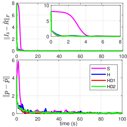
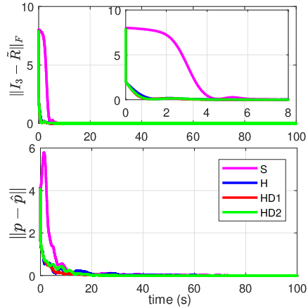
In this section, some simulation results are presented to illustrate the performance of the proposed hybrid pose observers (observer in Proposition 1, observer in Proposition 2 and observer in Theorem 2 and referred to,respectively, as H, HD1 and HD2). We refer to the smooth non-hybrid observer (i.e., the observer in Proposition 1 without the switching mechanism) as S.

As commonly used in practical applications, to avoid the bias estimation drift, in the presence of measurement noise, we introduce the following projection mechanism [24]:

ProjΔ​(b^,Γ​σ):={Γ​σ,if ​b^∈ΠΔ​ or ​∇b^𝒫⊤​Γ​σ≤0(I−ϱ⁡(b^)​Γ​∇b^𝒫​∇b^𝒫⊤∇b^𝒫⊤​Γ​∇b^𝒫)​Γ​σ,otherwise,\displaystyle\mathrm{Proj}_{\Delta}(\hat{b},\Gamma\sigma):=\begin{cases}\Gamma\sigma,&\text{if }\hat{b}\in\Pi_{\Delta}\text{ or }\nabla_{\hat{b}}\mathcal{P}^{\top}\Gamma\sigma\leq 0\\ \left(I-\varrho(\hat{b})\Gamma\frac{\nabla_{\hat{b}}\mathcal{P}\nabla_{\hat{b}}\mathcal{P}^{\top}}{\nabla_{\hat{b}}\mathcal{P}^{\top}\Gamma\nabla_{\hat{b}}\mathcal{P}}\right)\Gamma\sigma,&\text{otherwise}\end{cases},

where b^,σ∈ℝn,Γ∈ℝn×n\hat{b},\sigma\in\mathbb{R}^{n},\Gamma\in\mathbb{R}^{n\times n}, 𝒫⁡(b^):=‖b^‖−Δ\mathcal{P}(\hat{b}):=\|\hat{b}\|-\Delta, ΠΔ={b^|𝒫⁡(b^)≤0}\Pi_{\Delta}=\{\hat{b}|\mathcal{P}(\hat{b})\leq 0\}, ΠΔ,ϵ={b^|𝒫⁡(b^)≤ϵ}\Pi_{\Delta,\epsilon}=\{\hat{b}|\mathcal{P}(\hat{b})\leq\epsilon\} and ϱ⁡(b^):=min⁡{1,𝒫⁡(b^)/ϵ}\varrho(\hat{b}):=\min\{1,\mathcal{P}(\hat{b})/\epsilon\} for some positive parameters Δ\Delta and ϵ\epsilon. Given ‖b^​(0)‖<Δ\|\hat{b}(0)\|<\Delta, one can verify that the projection map ProjΔ\mathrm{Proj}_{\Delta} satisfies the following properties:

  • 1)

    ‖b^​(t)‖≤Δ+ϵ\|\hat{b}(t)\|\leq\Delta+\epsilon, for all t≥0t\geq 0 ;

  • 2)

    b~⊤​Γ−1​ProjΔ​(b^,Γ​σ)≤b~⊤​σ\tilde{b}^{\top}\Gamma^{-1}\mathrm{Proj}_{\Delta}(\hat{b},\Gamma\sigma)\leq\tilde{b}^{\top}\sigma;

  • 3)

    ‖ProjΔ​(b^,Γ​σ)‖≤‖Γ​σ‖\|\mathrm{Proj}_{\Delta}(\hat{b},\Gamma\sigma)\|\leq\|\Gamma\sigma\|.

Consider the three inertial vectors v1ℐ=[0​0​1]⊤,v2ℐ=[32​12​0]⊤,v3ℐ=[−12​32​0]⊤v_{1}^{\mathcal{I}}=[0~0~1]^{\top},v_{2}^{\mathcal{I}}=[\frac{\sqrt{3}}{2}~\frac{1}{2}~0]^{\top},v_{3}^{\mathcal{I}}=[-\frac{1}{2}~\frac{\sqrt{3}}{2}~0]^{\top} and one landmark pℐ=[22​22​2]⊤p^{\mathcal{I}}=[\frac{\sqrt{2}}{2}~\frac{\sqrt{2}}{2}~2]^{\top} are available. The initial pose for all the observers is taken as the identity i.e., g^​(0)=I4\hat{g}(0)=I_{4}. The system’s initial conditions are taken as follows: R​(0)=ℛa​(π,v)R(0)=\mathcal{R}_{a}(\pi,v) with v=[1​0​0]⊤∈ℰ⁡(Q)v=[1~0~0]^{\top}\in\mathcal{E}(Q) and p⁡(0)=[0​1​4]⊤p(0)=[0~1~4]^{\top}. The system is driven by the following linear and angular velocities: v⁡(t)=2​[cos⁡(t)​sin⁡(t)​0]⊤v(t)=2[\cos(t)~\sin(t)~0]^{\top}, ω⁡(t)=[−sin⁡(t)​cos⁡(t)​0]⊤\omega(t)=[-\sin(t)~\cos(t)~0]^{\top}. For the hybrid design, we choose θ∗=2​π/3\theta^{*}=2\pi/3, δ=1\delta=1 and 𝕌=𝔼⁡(Q)\mathbb{U}=\mathbb{E}(Q). The gain parameters involved in all the observers are taken as follows: ki=1,i=1,⋯,4k_{i}=1,i=1,\cdots,4, kβ=1,kω=1,kv=1k_{\beta}=1,k_{\omega}=1,k_{v}=1.

The simulation results are given in Fig. 2 - Fig. 3, from which one can clearly see the improved performance of the decoupled hybrid observer as compared to the non-decoupled hybrid observer and non-hybrid observer.
Refer to caption
(a) Rotation and position estimation errors.
Refer to caption
(b) Velocity-bias estimation errors.
Figure 2: Simulation results with non-noisy output measurements and constant velocity-bias ba=[−0.02​0.02​0.1​0.2−0.1​0.01]⊤b_{a}=[-0.02~0.02~~0.1~~0.2~-0.1~0.01]^{\top}.
Refer to caption
(a) Rotation and position estimation errors.
Refer to caption
(b) Velocity-bias estimation errors.
Figure 3: Simulation results with additive white Gaussian noise of variance 0.1 in the output measurements and time-varying velocity-bias ba​(t)=cos⁡(0.02​t)​[−0.02​0.02​0.1​0.2−0.1​0.01]⊤b_{a}(t)=\cos(0.02t)[-0.02~0.02~~0.1~~0.2~-0.1~0.01]^{\top}.

7 Conclusion

A globally exponentially stable hybrid pose and velocity-bias estimation scheme evolving on S​E​(3)×ℝ6SE(3)\times\mathbb{R}^{6} has been proposed. The proposed observer is formulated in terms of homogeneous output measurements of known inertial vectors and landmark points. It relies on an observer-state jump mechanism designed to avoid the undesired critical point while ensuring a decrease of the potential function in the flow and jump sets. Moreover, an auxiliary coordinate transformation is introduced on the landmark measurements, and a modified observer, leading to a decoupled rotational error dynamics from the translational dynamics, is proposed.

References

  • [1] M. Wang and A. Tayebi, “Globally asymptotically stable hybrid observers design on SE(3),” in Proceedings of the 56th IEEE Annual Conference on Decision and Control (CDC). IEEE, 2017, pp. 3033–3038.
  • [2] M. D. Shuster and S. D. Oh, “Three-axis attitude determination from vector observations,” Journal of Guidance and Control, vol. 4, pp. 70–77, 1981.
  • [3] J. L. Crassidis, F. L. Markley, and Y. Cheng, “Survey of nonlinear attitude estimation methods,” Journal of guidance, control, and dynamics, vol. 30, no. 1, pp. 12–28, 2007.
  • [4] A. Tayebi and S. McGilvray, “Attitude stabilization of a VTOL quadrotor aircraft,” IEEE Transactions on Control Systems Technology, vol. 14, no. 3, pp. 562–571, 2006.
  • [5] R. Mahony, T. Hamel, and J.-M. Pflimlin, “Nonlinear complementary filters on the special orthogonal group,” IEEE Transactions on automatic control, vol. 53, no. 5, pp. 1203–1218, 2008.
  • [6] H. Rehbinder and B. K. Ghosh, “Pose estimation using line-based dynamic vision and inertial sensors,” IEEE Transactions on Automatic Control, vol. 48, no. 2, pp. 186–199, 2003.
  • [7] T. Hamel and C. Samson, “Riccati observers for the non-stationary PnP problem,” IEEE Transactions on Automatic Control, vol. 63, no. 3, pp. 726–741, 2018.
  • [8] A. Moeini and M. Namvar, “Global attitude/position estimation using landmark and biased velocity measurements,” IEEE Transactions on Aerospace and Electronic Systems, vol. 52, no. 2, pp. 852–862, 2016.
  • [9] S. Bonnabel, P. Martin, and P. Rouchon, “Non-linear symmetry-preserving observers on Lie groups,” IEEE Transactions on Automatic Control, vol. 54, no. 7, pp. 1709–1713, 2009.
  • [10] C. Lageman, J. Trumpf, and R. Mahony, “Gradient-like observers for invariant dynamics on a Lie group,” IEEE Transactions on Automatic Control, vol. 55, no. 2, pp. 367–377, 2010.
  • [11] G. Baldwin, R. Mahony, J. Trumpf, T. Hamel, and T. Cheviron, “Complementary filter design on the special euclidean group S​E​(3)SE(3),” in Proceedings of the European Control Conference (ECC), 2007, pp. 3763–3770.
  • [12] M.-D. Hua, M. Zamani, J. Trumpf, R. Mahony, and T. Hamel, “Observer design on the special euclidean group S​E​(3)SE(3),” in Proceedings of the 50th IEEE Conference on Decision and Control and European Control Conference (CDC-ECC), 2011, pp. 8169–8175.
  • [13] J. F. Vasconcelos, R. Cunha, C. Silvestre, and P. Oliveira, “A nonlinear position and attitude observer on S​E​(3)SE(3) using landmark measurements,” Systems & Control Letters, vol. 59, no. 3, pp. 155–166, 2010.
  • [14] A. Khosravian, J. Trumpf, R. Mahony, and C. Lageman, “Observers for invariant systems on Lie groups with biased input measurements and homogeneous outputs,” Automatica, vol. 55, pp. 19–26, 2015.
  • [15] M.-D. Hua, T. Hamel, R. Mahony, and J. Trumpf, “Gradient-like observer design on the special euclidean group S​E​(3)SE(3) with system outputs on the real projective space,” in Proceedings of the 54th IEEE Annual Conference on Decision and Control (CDC),, 2015, pp. 2139–2145.
  • [16] C. G. Mayhew and A. R. Teel, “Hybrid control of rigid-body attitude with synergistic potential functions,” in Proceedings of the American Control Conference (ACC), 2011, pp. 287–292.
  • [17] T.-H. Wu, E. Kaufman, and T. Lee, “Globally asymptotically stable attitude observer on S​O​(3)SO(3),” in Proceedings of the 54th IEEE Conference on Decision and Control (CDC), 2015, pp. 2164–2168.
  • [18] S. Berkane and A. Tayebi, “Construction of synergistic potential functions on S​O​(3)SO(3) with application to velocity-free hybrid attitude stabilization,” IEEE Transactions on Automatic Control, vol. 62, no. 1, pp. 495–501, 2017.
  • [19] ——, “Attitude and gyro bias estimation using GPS and IMU measurements,” in Proceedings of the 56th IEEE Conference on Decision and Control (CDC). IEEE, 2017, pp. 2402–2407.
  • [20] S. Berkane, A. Abdessameud, and A. Tayebi, “Hybrid attitude and gyro-bias observer design on SO(3),” IEEE Transactions on Automatic Control, vol. 62, no. 11, pp. 6044–6050, 2017.
  • [21] R. Goebel, R. G. Sanfelice, and A. R. Teel, “Hybrid dynamical systems,” IEEE Control Systems, vol. 29, no. 2, pp. 28–93, 2009.
  • [22] ——, Hybrid Dynamical Systems: modeling, stability, and robustness. Princeton University Press, 2012.
  • [23] D. E. Koditschek, “The application of total energy as a Lyapunov function for mechanical control systems,” in Dynamics and Control of Multibody Systems, ser. Contemporary Mathematics, J. E. Marsden, P. S. Krishnaprasad, and J. C. Simo, Eds. Providence, RI: Amer. Math. Soc., vol. 97, pp. 131–157, 1989.
  • [24] P. A. Ioannou and J. Sun, Robust adaptive control. Prentice-Hall Englewood Cliffs, NJ, 1995.
  • [25] A. Tayebi, A. Roberts, and A. Benallegue, “Inertial vector measurements based velocity-free attitude stabilization,” IEEE Transactions on Automatic Control, vol. 58, no. 11, pp. 2893–2898, 2013.
  • [26] C. G. Mayhew and A. R. Teel, “Synergistic potential functions for hybrid control of rigid-body attitude,” in Proceedings of American Control Conference, 2011, pp. 875–880.
  • [27] S. Berkane, A. Abdessameud, and A. Tayebi, “Hybrid global exponential stabilization on S​O​(3)SO(3),” Automatica, vol. 81, pp. 279–285, 2017.

8 Appendices

8.1 Proof of Theorem 1

Let us consider the following real-valued function:

V⁡(x)=𝒰⁡(g~)+12​b~a​Γ−1​b~a,V(x)=\mathcal{U}(\tilde{g})+\frac{1}{2}\tilde{b}_{a}\Gamma^{-1}\tilde{b}_{a}, (86)

Taking the time derivative of VV, along the flows of trajectories of (27), one can show that

V˙\displaystyle\dot{V} =⟨∇g~𝒰​(g~),g~​(Adg^​(b~a−kβ​β))∧⟩g~−b~a⊤​Γ−1​Γ​σb\displaystyle=\left\langle\nabla_{\tilde{g}}\mathcal{U}(\tilde{g}),\tilde{g}(\mathrm{Ad}_{\hat{g}}(\tilde{b}_{a}-k_{\beta}\beta))^{\wedge}\right\rangle_{\tilde{g}}-\tilde{b}_{a}^{\top}\Gamma^{-1}\Gamma\sigma_{b}
≤⟨⟨g~−1​∇g~𝒰​(g~),(Adg^​(b~a−kβ​β​(g~)))∧⟩⟩−b~a⊤​σb\displaystyle\leq\langle\langle\tilde{g}^{-1}\nabla_{\tilde{g}}\mathcal{U}(\tilde{g}),(\mathrm{Ad}_{\hat{g}}(\tilde{b}_{a}-k_{\beta}\beta(\tilde{g})))^{\wedge}\rangle\rangle-\tilde{b}_{a}^{\top}\sigma_{b}
≤−kβ​⟨⟨g~−1​∇g~𝒰​(g~),(ψ⁡(g~−1​∇g~𝒰​(g~)))∧⟩⟩+⟨⟨Adg^∗​g~−1​∇g~𝒰​(g~),(b~a)∧⟩⟩−b~a⊤​σb​(g~)\displaystyle\leq-k_{\beta}\langle\langle\tilde{g}^{-1}\nabla_{\tilde{g}}\mathcal{U}(\tilde{g}),(\psi(\tilde{g}^{-1}\nabla_{\tilde{g}}\mathcal{U}(\tilde{g})))^{\wedge}\rangle\rangle+\langle\langle\mathrm{Ad}_{\hat{g}}^{*}~\tilde{g}^{-1}\nabla_{\tilde{g}}\mathcal{U}(\tilde{g}),(\tilde{b}_{a})^{\wedge}\rangle\rangle-\tilde{b}_{a}^{\top}\sigma_{b}(\tilde{g})
≤−kβ​‖ψ⁡(g~−1​∇g~𝒰​(g~))‖2+b~a⊤​Adg^∗​ψ​(g~−1​∇g~𝒰​(g~))−b~a⊤​σb\displaystyle\leq-k_{\beta}\|\psi(\tilde{g}^{-1}\nabla_{\tilde{g}}\mathcal{U}(\tilde{g}))\|^{2}+\tilde{b}_{a}^{\top}\mathrm{Ad}_{\hat{g}}^{*}\psi(\tilde{g}^{-1}\nabla_{\tilde{g}}\mathcal{U}(\tilde{g}))-\tilde{b}_{a}^{\top}\sigma_{b}
=−kβ​‖ψ⁡(g~−1​∇g~𝒰​(g~))‖2,\displaystyle=-k_{\beta}\|\psi(\tilde{g}^{-1}\nabla_{\tilde{g}}\mathcal{U}(\tilde{g}))\|^{2}, (87)

where we made use of (5) and Adg^​Adg^−1=I6\mathrm{Ad}_{\hat{g}}\mathrm{Ad}_{\hat{g}^{-1}}=I_{6}. Then, for any x∈ℱcx\in\mathcal{F}_{c}, VV is non-increasing along the flows of (27). Using the fact ℱc∪𝒥c=𝒮\mathcal{F}_{c}\cup\mathcal{J}_{c}=\mathcal{S} and the definitions of 𝒳𝒰\mathcal{X}_{\mathcal{U}} and 𝒥c\mathcal{J}_{c}, from (29) one has 𝒳𝒰×ℝ6×S​E​(3)×ℝ6×ℝ≥0⊆𝒥c\mathcal{X}_{\mathcal{U}}\times\mathbb{R}^{6}\times SE(3)\times\mathbb{R}^{6}\times\mathbb{R}_{\geq 0}\subseteq\mathcal{J}_{c}.

For any x∈𝒥cx\in\mathcal{J}_{c}, one can show that

V⁡(x+)−V⁡(x)\displaystyle V(x^{+})-V(x) =𝒰⁡(g~+)−𝒰⁡(g~)\displaystyle=\mathcal{U}(\tilde{g}^{+})-\mathcal{U}(\tilde{g})
≤mingq∈ℚ⁡𝒰⁡(g~​gq)−𝒰⁡(g~)≤−δ,\displaystyle\leq\min_{g_{q}\in\mathbb{Q}}\mathcal{U}(\tilde{g}g_{q})-\mathcal{U}(\tilde{g})\leq-\delta, (88)

which implies that VV is strictly decreasing over the jumps of (27). Thus, in view of (87) and (88), one can easily show that

0<V⁡(x⁡(t,j))≤V⁡(x⁡(0,0))−j​δ,0<V(x(t,j))\leq V(x(0,0))-j\delta, (89)

which leads to 0≤j≤Jmax:=⌈V⁡(x⁡(0,0))/δ⌉0\leq j\leq J_{\max}:=\left\lceil{V(x(0,0))}/{\delta}~\right\rceil with ⌈⋅⌉\lceil\cdot\rceil denoting the ceiling function. This implies that the number of jumps is finite.

To show exponential stability, let us consider the following Lyapunov function candidate:

ℒ⁡(x)=V⁡(x)−z⊤​U​b~a,\displaystyle\mathcal{L}(x)=V(x)-z^{\top}U\tilde{b}_{a}, (90)

where U:=diag​(μ1​I3,μ2​I3)U:=\text{diag}(\mu_{1}I_{3},\mu_{2}I_{3}) with μ1,μ2>0\mu_{1},\mu_{2}>0 and z:=[ψa​(R~)⊤​R^,p~⊤​R]⊤z:=[\psi_{a}(\tilde{R})^{\top}\hat{R},\tilde{p}^{\top}R]^{\top}. Let e:=[|g~|I,‖b~ω‖,‖b~v‖]⊤e:=[|\tilde{g}|_{I},\|\tilde{b}_{\omega}\|,\|\tilde{b}_{v}\|]^{\top} and eie_{i} be the ii-th elements of ee. From (28), one obtains

ℒ\displaystyle\mathcal{L} ≤α2​e12+1kω​e22+1kv​e32+e1​(2​μ12​e2+μ2​e3)\displaystyle\leq\alpha_{2}e_{1}^{2}+\frac{1}{k_{\omega}}e_{2}^{2}+\frac{1}{k_{v}}e_{3}^{2}+e_{1}(\frac{\sqrt{2}\mu_{1}}{2}e_{2}+\mu_{2}e_{3})
ℒ\displaystyle\mathcal{L} ≥α1​e12+1kω​e22+1kv​e32−e1​(2​μ12​e2+μ2​e3),\displaystyle\geq\alpha_{1}e_{1}^{2}+\frac{1}{k_{\omega}}e_{2}^{2}+\frac{1}{k_{v}}e_{3}^{2}-e_{1}(\frac{\sqrt{2}\mu_{1}}{2}e_{2}+\mu_{2}e_{3}),

which implies

e⊤​[α1−24​μ1−12​μ2−24​μ11kω0−12​μ201kv]⏟P1​e≤ℒ⁡(x)≤e⊤​[α224​μ112​μ224​μ11kω012​μ201kv]⏟P2​e.\displaystyle e^{\top}\underbrace{\begin{bmatrix}\alpha_{1}&\frac{-\sqrt{2}}{4}\mu_{1}&\frac{-1}{2}\mu_{2}\\ \frac{-\sqrt{2}}{4}\mu_{1}&\frac{1}{k_{\omega}}&0\\ \frac{-1}{2}\mu_{2}&0&\frac{1}{k_{v}}\end{bmatrix}}_{P_{1}}e\leq\mathcal{L}(x)\leq e^{\top}\underbrace{\begin{bmatrix}\alpha_{2}&\frac{\sqrt{2}}{4}\mu_{1}&\frac{1}{2}\mu_{2}\\ \frac{\sqrt{2}}{4}\mu_{1}&\frac{1}{k_{\omega}}&0\\ \frac{1}{2}\mu_{2}\ &0&\frac{1}{k_{v}}\end{bmatrix}}_{P_{2}}e.

Using the fact |x|𝒜¯2=|g~|I2+‖b~a‖2=‖e‖2,|x|_{\bar{\mathcal{A}}}^{2}=|\tilde{g}|_{I}^{2}+\|\tilde{b}_{a}\|^{2}=\|e\|^{2}, one obtains the following inequalities:

λminP1​|x|𝒜¯2≤ℒ⁡(x)≤λmaxP2​|x|𝒜¯2.\lambda_{\min}^{P_{1}}|x|_{\bar{\mathcal{A}}}^{2}\leq\mathcal{L}(x)\leq\lambda_{\max}^{P_{2}}|x|_{\bar{\mathcal{A}}}^{2}. (91)

Let ψR~:=ψa​(R~)\psi_{\tilde{R}}:=\psi_{a}(\tilde{R}). One verifies that ‖ψR~‖2≤12​‖I3−R~‖F2≤4\|\psi_{\tilde{R}}\|^{2}\leq\frac{1}{2}\|I_{3}-\tilde{R}\|_{F}^{2}\leq 4 and ‖ψR~‖2≤12​|g~|I2\|\psi_{\tilde{R}}\|^{2}\leq\frac{1}{2}|\tilde{g}|_{I}^{2}. From (27), one has

R~˙\displaystyle\dot{\tilde{R}}~~ =R~​(−kβ​ψω+R^​b~ω)×,\displaystyle=\tilde{R}(-k_{\beta}\psi_{\omega}+\hat{R}\tilde{b}_{\omega})^{\times}, (92)
p~˙\displaystyle\dot{\tilde{p}}~~ =R~​(−kβ​ψv+p^×​R^​b~ω+R^​b~v),\displaystyle=\tilde{R}(-k_{\beta}\psi_{v}+\hat{p}^{\times}\hat{R}\tilde{b}_{\omega}+\hat{R}\tilde{b}_{v}), (93)
ψ˙R~\displaystyle\dot{\psi}_{\tilde{R}} =E⁡(R~)​(−kβ​ψω+R^​b~ω),\displaystyle=E(\tilde{R})(-k_{\beta}\psi_{\omega}+\hat{R}\tilde{b}_{\omega}), (94)

where E⁡(R~):=12​(tr⁡(R~)−R~⊤)E(\tilde{R}):=\frac{1}{2}(\mathrm{tr}(\tilde{R})-\tilde{R}^{\top}). The arguments of ψ\psi have been omitted for simplicity, and ψω,ψv\psi_{\omega},\psi_{v} are given by ψ:=[ψω⊤,ψv⊤]⊤\psi:=[\psi_{\omega}^{\top},\psi_{v}^{\top}]^{\top}. From Lemma 2 in [20], one has ‖E⁡(R~)‖F≤3\|E(\tilde{R})\|_{F}\leq\sqrt{3} and v⊤​(I3−E⁡(R~))​v≤14​‖I3−R~‖F2​‖v‖2≤22​‖I3−R~‖F​‖v‖2≤22​|g~|I​‖v‖2v^{\top}(I_{3}-E(\tilde{R}))v\leq\frac{1}{4}\|I_{3}-\tilde{R}\|_{F}^{2}\|v\|^{2}\leq\frac{\sqrt{2}}{2}\|I_{3}-\tilde{R}\|_{F}\|v\|^{2}\leq\frac{\sqrt{2}}{2}|\tilde{g}|_{I}\|v\|^{2} for all v∈ℝ3v\in\mathbb{R}^{3}. Define the constants cω:=supt≥0‖ω⁡(t)‖c_{\omega}:=\sup_{t\geq 0}\|\omega(t)\| and cp:=supt≥0‖p⁡(t)‖c_{p}:=\sup_{t\geq 0}\|p(t)\|. Since b~ω\tilde{b}_{\omega} is bounded both in the flow and jump sets, there exists a constant cbω:=sup(t,j)⪰(0,0)‖b~ω​(t,j)‖c_{b_{\omega}}:=\sup_{(t,j)\succeq(0,0)}\|\tilde{b}_{\omega}(t,j)\|. In view of (92)-(94), the time-derivative of the cross term 𝔛:=z⊤​U​b~a=−μ1​b~ω⊤​R^⊤​ψR~−μ2​p~⊤​R​b~v\mathfrak{X}:=z^{\top}U\tilde{b}_{a}=-\mu_{1}\tilde{b}_{\omega}^{\top}\hat{R}^{\top}\psi_{\tilde{R}}-\mu_{2}\tilde{p}^{\top}R\tilde{b}_{v} is obtained as

𝔛˙\displaystyle\dot{\mathfrak{X}} =−z˙⊤​U​b~a−z⊤​U​b~˙a\displaystyle=-\dot{z}^{\top}U\tilde{b}_{a}-z^{\top}U\dot{\tilde{b}}_{a}
=−μ1​b~ω⊤​(R^˙⊤​ψR~+R^⊤​ψ˙a​(R~))−μ2​b~v⊤​(R⊤​p~˙+R˙⊤​p~)−z⊤​U​b~˙a\displaystyle=-\mu_{1}\tilde{b}_{\omega}^{\top}(\dot{\hat{R}}^{\top}\psi_{\tilde{R}}+\hat{R}^{\top}\dot{\psi}_{a}(\tilde{R}))-\mu_{2}\tilde{b}_{v}^{\top}(R^{\top}\dot{\tilde{p}}+\dot{R}^{\top}\tilde{p})-z^{\top}U\dot{\tilde{b}}_{a}
=μ1​b~ω⊤​(ω−b~ω+kβ​ψω)×​R^⊤​ψR~−μ1​b~ω⊤​R^⊤​E​(R~)​(−kβ​ψω+R^​b~ω)+μ2​b~v⊤​(ω)×​R⊤​p~\displaystyle=\mu_{1}\tilde{b}_{\omega}^{\top}(\omega-\tilde{b}_{\omega}+k_{\beta}\psi_{\omega})^{\times}\hat{R}^{\top}\psi_{\tilde{R}}-\mu_{1}\tilde{b}_{\omega}^{\top}\hat{R}^{\top}E(\tilde{R})(-k_{\beta}\psi_{\omega}+\hat{R}\tilde{b}_{\omega})+\mu_{2}\tilde{b}_{v}^{\top}(\omega)^{\times}R^{\top}\tilde{p}
−μ2b~v⊤R^⊤(−kβψv+p^×R^b~ω+R^b~v)+z⊤UΓAdg∗Adg~−1∗ψ∥\displaystyle~~~-\mu_{2}\tilde{b}_{v}^{\top}\hat{R}^{\top}(-k_{\beta}\psi_{v}+\hat{p}^{\times}\hat{R}\tilde{b}_{\omega}+\hat{R}\tilde{b}_{v})+z^{\top}U\Gamma\mathrm{Ad}_{g}^{*}\mathrm{Ad}_{\tilde{g}^{-1}}^{*}\psi\|
≤−μ1​‖b~ω‖2−μ2​‖b~v‖2+μ1​cω​‖ψR~‖​‖b~ω​‖+μ1​kβ‖​b~ω‖​‖ψω‖​‖ψR~‖\displaystyle\leq-\mu_{1}\|\tilde{b}_{\omega}\|^{2}-\mu_{2}\|\tilde{b}_{v}\|^{2}+\mu_{1}c_{\omega}\|\psi_{\tilde{R}}\|\|\tilde{b}_{\omega}\|+\mu_{1}k_{\beta}\|\tilde{b}_{\omega}\|\|\psi_{\omega}\|\|\psi_{\tilde{R}}\|
+μ1​b~ω⊤​R^⊤​(I3−E⁡(R~))​R^​b~ω+μ1​kβ​‖b~ω​‖‖E⁡(R~)‖F​‖ψω​‖+μ2​cω‖​b~v‖‖​p~‖\displaystyle~~~+\mu_{1}\tilde{b}_{\omega}^{\top}\hat{R}^{\top}(I_{3}-E(\tilde{R}))\hat{R}\tilde{b}_{\omega}+\mu_{1}k_{\beta}\|\tilde{b}_{\omega}\|\|E(\tilde{R})\|_{F}\|\psi_{\omega}\|+\mu_{2}c_{\omega}\|\tilde{b}_{v}\|\|\tilde{p}\|
+μ2​kβ​‖b~v​‖‖ψv​‖+μ2​cbω​‖b~v​‖‖p~​‖+μ2​cp​‖b~v‖‖​b~ω​‖+kΓ‖​U‖2‖​z‖‖​Adg∗‖F‖​Adg~−1∗​ψ‖\displaystyle~~~+\mu_{2}k_{\beta}\|\tilde{b}_{v}\|\|\psi_{v}\|+\mu_{2}c_{b_{\omega}}\|\tilde{b}_{v}\|\|\tilde{p}\|+\mu_{2}c_{p}\|\tilde{b}_{v}\|\|\tilde{b}_{\omega}\|+k_{\Gamma}\|U\|_{2}\|z\|\|\mathrm{Ad}_{g}^{*}\|_{F}\|\mathrm{Ad}_{\tilde{g}^{-1}}^{*}\psi\|
≤−μ1​‖b~ω‖2−μ2​‖b~v‖2+2​α4​μ1​kβ​‖b~ω‖​|g~|I+22​μ1​cω|​g~|I​‖b~ω‖\displaystyle\leq-\mu_{1}\|\tilde{b}_{\omega}\|^{2}-\mu_{2}\|\tilde{b}_{v}\|^{2}+2\sqrt{\alpha_{4}}\mu_{1}k_{\beta}\|\tilde{b}_{\omega}\||\tilde{g}|_{I}+{\textstyle\frac{\sqrt{2}}{2}}\mu_{1}c_{\omega}|\tilde{g}|_{I}\|\tilde{b}_{\omega}\|
+22​μ1​cbω​|g~|I​‖b~ω‖+3​α4​μ1​kβ​‖b~ω​‖|g~|I+μ2​cω​‖b~v‖|​g~|I+α4​μ2​kβ‖​b~v‖|g~|I\displaystyle~~~+{\textstyle\frac{\sqrt{2}}{2}}\mu_{1}c_{b_{\omega}}|\tilde{g}|_{I}\|\tilde{b}_{\omega}\|+\sqrt{3\alpha_{4}}\mu_{1}k_{\beta}\|\tilde{b}_{\omega}\||\tilde{g}|_{I}+\mu_{2}c_{\omega}\|\tilde{b}_{v}\||\tilde{g}|_{I}+\sqrt{\alpha_{4}}\mu_{2}k_{\beta}\|\tilde{b}_{v}\||\tilde{g}|_{I}
+μ2​cbω​‖b~v‖​|g~|I+μ2​cp​‖b~v‖​‖b~ω‖+kΓ​cg​α5​(u1+u2)​|g~|I2\displaystyle~~~+\mu_{2}c_{b_{\omega}}\|\tilde{b}_{v}\||\tilde{g}|_{I}+\mu_{2}c_{p}\|\tilde{b}_{v}\|\|\tilde{b}_{\omega}\|+k_{\Gamma}c_{g}\sqrt{\alpha_{5}}(u_{1}+u_{2})|\tilde{g}|_{I}^{2}
≤−μ1​‖b~ω‖2−μ2​‖b~v‖2+μ1​(22​cω+2​α4​kβ+22​cbω+3​α4​kβ)​|g~|I​‖b~ω‖\displaystyle\leq-\mu_{1}\|\tilde{b}_{\omega}\|^{2}-\mu_{2}\|\tilde{b}_{v}\|^{2}+\mu_{1}({\textstyle\frac{\sqrt{2}}{2}}c_{\omega}+2\sqrt{\alpha_{4}}k_{\beta}+{\textstyle\frac{\sqrt{2}}{2}}c_{b_{\omega}}+\sqrt{3\alpha_{4}}k_{\beta})|\tilde{g}|_{I}\|\tilde{b}_{\omega}\|
+μ2​(cω+α4​kβ+cbω)​‖b~v‖​|g~|I+μ2​cp​‖b~v‖​‖b~ω‖+kΓ​cg​α5​(u1+u2)​|g~|I2,\displaystyle~~~+\mu_{2}(c_{\omega}+\sqrt{\alpha_{4}}k_{\beta}+c_{b_{\omega}})\|\tilde{b}_{v}\||\tilde{g}|_{I}+\mu_{2}c_{p}\|\tilde{b}_{v}\|\|\tilde{b}_{\omega}\|+k_{\Gamma}c_{g}\sqrt{\alpha_{5}}(u_{1}+u_{2})|\tilde{g}|_{I}^{2},

where kΓ:=‖Γ‖F,cg:=‖Adg∗‖F=6+2​cp2k_{\Gamma}:=\|\Gamma\|_{F},c_{g}:=\|\mathrm{Ad}_{g}^{*}\|_{F}=\sqrt{6+2c_{p}^{2}}, and the following facts have been used: |g~|I2=‖I3−R~‖2+‖p~‖2|\tilde{g}|_{I}^{2}=\|I_{3}-\tilde{R}\|^{2}+\|\tilde{p}\|^{2}, ‖p^‖=‖R~⊤​(p−p~)‖≤cp+‖p~‖\|\hat{p}\|=\|\tilde{R}^{\top}(p-\tilde{p})\|\leq c_{p}+\|\tilde{p}\|, ‖ψω‖2+‖ψv‖2≤α4​|g~|I2\|\psi_{\omega}\|^{2}+\|\psi_{v}\|^{2}\leq\alpha_{4}|\tilde{g}|_{I}^{2}, ‖z‖=‖ψR~‖+‖p~‖≤|g~|I\|z\|=\|\psi_{\tilde{R}}\|+\|\tilde{p}\|\leq|\tilde{g}|_{I}, ‖U‖2≤(μ1+μ2)\|U\|_{2}\leq(\mu_{1}+\mu_{2}) and Eq. (30). Let c1:=22​cω+2​kβ​α4+2​cbω2+kβ​3​α4,c2:=kβ​α4+cbω+cω,c3:=kΓ​α5​cgc_{1}:=\frac{\sqrt{2}}{2}c_{\omega}+2k_{\beta}\sqrt{\alpha_{4}}+\frac{\sqrt{2}c_{b_{\omega}}}{2}+k_{\beta}\sqrt{3\alpha_{4}},c_{2}:=k_{\beta}\sqrt{\alpha_{4}}+c_{b_{\omega}}+c_{\omega},c_{3}:=k_{\Gamma}\sqrt{\alpha_{5}}c_{g}. Then, the time-derivative of 𝔛\mathfrak{X} satisfies

𝔛˙\displaystyle\dot{\mathfrak{X}} ≤−μ1​‖b~ω‖2−μ2​‖b~v‖2+μ1​c1​‖b~ω‖​|g~|I+μ2​c2​‖b~v‖|g~|I\displaystyle\leq-\mu_{1}\|\tilde{b}_{\omega}\|^{2}-\mu_{2}\|\tilde{b}_{v}\|^{2}+\mu_{1}c_{1}\|\tilde{b}_{\omega}\||\tilde{g}|_{I}+\mu_{2}c_{2}\|\tilde{b}_{v}\||\tilde{g}|_{I}
+(μ1​c3+μ2​c3)​|g~|I2+μ2​cp​‖b~v‖​‖b~ω‖,\displaystyle~~~+(\mu_{1}c_{3}+\mu_{2}c_{3})|\tilde{g}|_{I}^{2}+\mu_{2}c_{p}\|\tilde{b}_{v}\|\|\tilde{b}_{\omega}\|, (95)

Consequently, in view of (87) and (95), one obtains

ℒ˙\displaystyle\dot{\mathcal{L}} ≤−2​kβ​α3​e12+(μ1​c3+μ2​c3)​e12−μ1​‖b~ω‖2−μ2​‖b~v‖2\displaystyle\leq-2k_{\beta}\alpha_{3}e_{1}^{2}+(\mu_{1}c_{3}+\mu_{2}c_{3})e_{1}^{2}-\mu_{1}\|\tilde{b}_{\omega}\|^{2}-\mu_{2}\|\tilde{b}_{v}\|^{2}
+μ1​c1​‖b~ω‖​e1+μ2​c2​‖b~v‖​e1+μ2​cp​‖b~v‖​‖b~ω‖\displaystyle~~~+\mu_{1}c_{1}\|\tilde{b}_{\omega}\|e_{1}+\mu_{2}c_{2}\|\tilde{b}_{v}\|e_{1}+\mu_{2}c_{p}\|\tilde{b}_{v}\|\|\tilde{b}_{\omega}\|
=−e⊤​[2​kβ​α3−μ1​c3−μ2​c3−12​μ1​c1−12​μ2​c2−12​μ1​c1μ1−12​μ2​cp−12​μ2​c2−12​μ2​cpμ2]​e\displaystyle=-e^{\top}\begin{bmatrix}2k_{\beta}\alpha_{3}-\mu_{1}c_{3}-\mu_{2}c_{3}&-\frac{1}{2}\mu_{1}c_{1}&-\frac{1}{2}\mu_{2}c_{2}\\ -\frac{1}{2}\mu_{1}c_{1}&\mu_{1}&-\frac{1}{2}\mu_{2}c_{p}\\ -\frac{1}{2}\mu_{2}c_{2}&-\frac{1}{2}\mu_{2}c_{p}&\mu_{2}\end{bmatrix}e
=−e12⊤​P31​e12−e13⊤​P32​e13−e23⊤​P33​e23,\displaystyle=-e_{12}^{\top}P_{31}e_{12}-e_{13}^{\top}P_{32}e_{13}-e_{23}^{\top}P_{33}e_{23},

where ei​j:=[ei,ej]⊤,i,j∈{1,2,3}e_{ij}:=[e_{i},e_{j}]^{\top},i,j\in\{1,2,3\} with eie_{i} denoting the ii-th elements of ee, and

P31\displaystyle P_{31} :=[kβ​α3−μ1​c3−12​μ1​c1−12​μ1​c112​μ1],P32:=[kβ​α3−μ2​c3−12​μ2​c2−12​μ2​c212​μ2],P33:=[12​μ1−12​μ2​cp−12​μ2​cp12​μ2].\displaystyle:=\begin{bmatrix}k_{\beta}\alpha_{3}-\mu_{1}c_{3}&-\frac{1}{2}\mu_{1}c_{1}\\ -\frac{1}{2}\mu_{1}c_{1}&\frac{1}{2}\mu_{1}\end{bmatrix},P_{32}:=\begin{bmatrix}k_{\beta}\alpha_{3}-\mu_{2}c_{3}&-\frac{1}{2}\mu_{2}c_{2}\\ -\frac{1}{2}\mu_{2}c_{2}&\frac{1}{2}\mu_{2}\end{bmatrix},P_{33}:=\begin{bmatrix}\frac{1}{2}\mu_{1}&-\frac{1}{2}\mu_{2}c_{p}\\ -\frac{1}{2}\mu_{2}c_{p}&\frac{1}{2}\mu_{2}\end{bmatrix}.

To guarantee that the matrices P1,P2,P31,P32P_{1},P_{2},P_{31},P_{32} and P33P_{33} are positive definite, the μ1\mu_{1} and μ2\mu_{2} are chosen as follows:

μ1\displaystyle\mu_{1} <2​α1kω,μ2​<2​α1kv for ​P1,P2>​0\displaystyle<\frac{2\sqrt{\alpha_{1}}}{\sqrt{k_{\omega}}},\hskip 9.24994pt~~\mu_{2}<\frac{\sqrt{2\alpha_{1}}}{\sqrt{k_{v}}}~~~~~~~~~~\text{ for }P_{1},P_{2}>0
μ1\displaystyle\mu_{1} <kβ​α3c3+14​c12,μ2​<kβ​α3c3+14​c22 for ​P31,P32>​0\displaystyle<\frac{k_{\beta}\alpha_{3}}{c_{3}+\frac{1}{4}c_{1}^{2}},\hskip 9.24994pt\mu_{2}<\frac{k_{\beta}\alpha_{3}}{c_{3}+\frac{1}{4}c_{2}^{2}}~~~~~~\text{ for }P_{31},P_{32}>0
μ2\displaystyle\mu_{2} <1cp2​μ1 for ​P33>​0\displaystyle<\frac{1}{c_{p}^{2}}\mu_{1}~~~~~~~~~~~~~~~~~~~~~~~~~~~~~~~~\text{ for }P_{33}>0

which are equivalent to

0<μ1<min⁡{2​α1kω,kβ​α3c3+14​c12}\displaystyle 0<\mu_{1}<\min\left\{\frac{2\sqrt{\alpha_{1}}}{\sqrt{k_{\omega}}},\frac{k_{\beta}\alpha_{3}}{c_{3}+\frac{1}{4}c_{1}^{2}}\right\}
0<μ2<min⁡{2​α1kv,kβ​α3c3+14​c22,1cp2​μ1}.\displaystyle 0<\mu_{2}<\min\left\{\frac{\sqrt{2\alpha_{1}}}{\sqrt{k_{v}}},\frac{k_{\beta}\alpha_{3}}{c_{3}+\frac{1}{4}c_{2}^{2}},\frac{1}{c_{p}^{2}}\mu_{1}\right\}.

One concludes that

ℒ˙​(x)≤−λF​ℒ​(x),x∈ℱc,\dot{\mathcal{L}}(x)\leq-\lambda_{F}\mathcal{L}(x),\hskip 9.24994ptx\in\mathcal{F}_{c}, (96)

with λF:=min⁡{λminP31,λminP32,λminP33}/λmaxP2\lambda_{F}:=\min\{\lambda_{\min}^{P_{31}},\lambda_{\min}^{P_{32}},\lambda_{\min}^{P_{33}}\}/\lambda_{\max}^{P_{2}}. On the other hand, from (87) and (88), it is clear that b~a\tilde{b}_{a} is bounded in the flow and jump sets. Hence, there exists a constant cba:=sup(t,j)⪰(0,0)‖b~a​(t,j)‖c_{b_{a}}:=\sup_{(t,j)\succeq(0,0)}\|\tilde{b}_{a}(t,j)\|. Let gq=𝒯⁡(Rq,pq)∈ℚg_{q}=\mathcal{T}(R_{q},p_{q})\in\mathbb{Q}. Using the facts: R~+=R~​Rq\tilde{R}^{+}=\tilde{R}R_{q} and p~+=p~+R~​pq\tilde{p}^{+}=\tilde{p}+\tilde{R}p_{q}, one has

‖z+−z‖\displaystyle\|z^{+}-z\| =‖[(R^+)⊤​ψa​(R~+)−R^⊤​ψa​(R~)R⊤​p~+−R⊤​p~]‖\displaystyle=\left\|\begin{bmatrix}(\hat{R}^{+})^{\top}\psi_{a}(\tilde{R}^{+})-\hat{R}^{\top}\psi_{a}(\tilde{R})\\ R^{\top}\tilde{p}^{+}-R^{\top}\tilde{p}\end{bmatrix}\right\|
≤‖Rq​ψa​(R~​Rq)−ψa​(R~)‖+‖p~+−p~‖≤4+‖pq‖,\displaystyle\leq\|R_{q}\psi_{a}(\tilde{R}R_{q})-\psi_{a}(\tilde{R})\|+\|\tilde{p}^{+}-\tilde{p}\|\leq 4+\|p_{q}\|,

which implies

ℒ⁡(x+)−ℒ⁡(x)\displaystyle\mathcal{L}(x^{+})-\mathcal{L}(x) =V⁡(x+)−V⁡(x)+(z+)⊤​U​b~a−z⊤​U​b~a\displaystyle=V(x^{+})-V(x)+(z^{+})^{\top}U\tilde{b}_{a}-z^{\top}U\tilde{b}_{a}
≤−δ+(μ1+μ2)​c4,\displaystyle\leq-\delta+(\mu_{1}+\mu_{2})c_{4},

where c4:=(4+‖pq‖)​cbac_{4}:=(4+\|p_{q}\|)c_{b_{a}}. Choosing μ1\mu_{1} and μ2\mu_{2} such that

0<μ1<min⁡{2​α1kω,kβ​α3c3+14​c12,δ2​c4},\displaystyle 0<\mu_{1}<\min\left\{\frac{2\sqrt{\alpha_{1}}}{\sqrt{k_{\omega}}},\frac{k_{\beta}\alpha_{3}}{c_{3}+\frac{1}{4}c_{1}^{2}},\frac{\delta}{2c_{4}}\right\},
0<μ2<min⁡{2​α1kv,kβ​α3c3+14​c22,1cp2​μ1,μ1},\displaystyle 0<\mu_{2}<\min\left\{\frac{\sqrt{2\alpha_{1}}}{\sqrt{k_{v}}},\frac{k_{\beta}\alpha_{3}}{c_{3}+\frac{1}{4}c_{2}^{2}},\frac{1}{c_{p}^{2}}\mu_{1},\mu_{1}\right\},

there exists a constant δ∗:=δ−2​μ1​c4>0\delta^{*}:=\delta-2\mu_{1}c_{4}>0 such that one has

ℒ⁡(x+)≤ℒ⁡(x)−δ∗,x∈𝒥c.\mathcal{L}(x^{+})\leq\mathcal{L}(x)-\delta^{*},\hskip 9.24994ptx\in\mathcal{J}_{c}. (97)

In view of (91), (96) and (97), one concludes

λminP1|x|𝒜¯2≤ℒ⁡(x)≤λmaxP2|x|𝒜¯2,,x∈𝒮\displaystyle\lambda_{\min}^{P_{1}}|x|_{\bar{\mathcal{A}}}^{2}\leq\mathcal{L}(x)\leq\lambda_{\max}^{P_{2}}|x|_{\bar{\mathcal{A}}}^{2},\hskip 9.24994pt,x\in\mathcal{S}
ℒ˙​(x)≤−λF​ℒ​(x),x∈ℱc,\displaystyle\dot{\mathcal{L}}(x)\leq-\lambda_{F}\mathcal{L}(x),\hskip 9.24994ptx\in\mathcal{F}_{c},
ℒ⁡(x+)≤exp⁡(−λJ)​ℒ​(x),x∈𝒥c,\displaystyle\mathcal{L}(x^{+})\leq\exp(-\lambda_{J})\mathcal{L}(x),\hskip 9.24994ptx\in\mathcal{J}_{c},

with λJ:=−ln⁡(1−δ∗/ℒ⁡(0,0))\lambda_{J}:=-\ln(1-\delta^{*}/\mathcal{L}(0,0)). Consequently, one obtains

ℒ⁡(t,j)≤exp⁡(−2​λ​(t+j))​ℒ​(0,0),\mathcal{L}(t,j)\leq\exp(-2\lambda(t+j))\mathcal{L}(0,0), (98)

where λ:=12​min⁡{λF,λJ}\lambda:=\frac{1}{2}\min\{\lambda_{F},\lambda_{J}\}. From (91) and (98), for each (t,j)∈dom​x(t,j)\in\text{dom}x one has

|x⁡(t,j)|𝒜¯≤k​exp⁡(−λ⁡(t+j))|x⁡(0,0)|𝒜¯,|x(t,j)|_{\bar{\mathcal{A}}}\leq k\exp\left(-\lambda(t+j)\right)|x(0,0)|_{\bar{\mathcal{A}}}, (99)

where k:=λmaxP2/λminP1k:=\sqrt{\scalebox{0.8}{\mbox{$\displaystyle{\lambda_{\max}^{P_{2}}}/{\lambda_{\min}^{P_{1}}}$}}}. Since ℱc∪𝒥c=𝒮\mathcal{F}_{c}\cup\mathcal{J}_{c}=\mathcal{S}, the number of jumps if finite and there is no finite escape-time, one concludes that the solution to the hybrid system ℋ\mathcal{H} is complete as per Proposition 2.10 in [22]. This completes the proof.

8.2 Proof of Lemma 1

From the definition of matrix 𝔸\mathbb{A} in (32), one can show that

𝔸\displaystyle\mathbb{A} =∑i=1nki​ri​ri⊤=[∑i=1n1ki​piℐ​(piℐ)⊤+∑j=1n2kj+n1​vjℐ​(vjℐ)⊤∑i=1n1ki​piℐ∑i=1n1ki​(piℐ)⊤∑i=1n1ki],\displaystyle=\sum_{i=1}^{n}k_{i}r_{i}r_{i}^{\top}=\begin{bmatrix}\sum_{i=1}^{n_{1}}k_{i}p_{i}^{\mathcal{I}}(p_{i}^{\mathcal{I}})^{\top}+\sum_{j=1}^{n_{2}}k_{j+n_{1}}v_{j}^{\mathcal{I}}(v_{j}^{\mathcal{I}})^{\top}&\sum_{i=1}^{n_{1}}k_{i}p_{i}^{\mathcal{I}}\\ \sum_{i=1}^{n_{1}}k_{i}(p_{i}^{\mathcal{I}})^{\top}&\sum_{i=1}^{n_{1}}k_{i}\end{bmatrix},

which implies:

A\displaystyle A :=∑i=1n1ki​piℐ​(piℐ)⊤+∑j=1n2kj+n1​vjℐ​(vjℐ)⊤,\displaystyle:=\sum_{i=1}^{n_{1}}k_{i}p_{i}^{\mathcal{I}}(p_{i}^{\mathcal{I}})^{\top}+\sum_{j=1}^{n_{2}}k_{j+n_{1}}v_{j}^{\mathcal{I}}(v_{j}^{\mathcal{I}})^{\top},
b\displaystyle b :=∑i=1n1ki​piℐ,d:=∑i=1n1ki.\displaystyle:=\sum_{i=1}^{n_{1}}k_{i}p_{i}^{\mathcal{I}},\hskip 18.49988ptd:=\sum_{i=1}^{n_{1}}k_{i}.

From Assumption 1, there exists at least one gain parameter ki>0k_{i}>0 for all i=1,2,⋯,n1i=1,2,\cdots,n_{1}. Hence, one has d>0d>0. Let αi=ki/(∑i=1n1ki)\alpha_{i}=k_{i}/(\sum_{i=1}^{n_{1}}k_{i}), and it is easy to verify that pcℐ=∑i=1n1αi​piℐ=b​d−1.p^{\mathcal{I}}_{c}=\sum_{i=1}^{n_{1}}\alpha_{i}p^{\mathcal{I}}_{i}=bd^{-1}. In view of (18) and (32), one has

Q\displaystyle Q =A−b​b⊤​d−1\displaystyle=A-bb^{\top}d^{-1}
=∑i=1n1ki​piℐ​(piℐ)⊤+∑i=1n2kj+n1​viℐ​(viℐ)⊤−(∑i=1n1ki​piℐ)​(∑i=1n1ki​piℐ)⊤​(∑i=1n1ki)−1\displaystyle=\sum_{i=1}^{n_{1}}k_{i}p_{i}^{\mathcal{I}}\left(p_{i}^{\mathcal{I}}\right)^{\top}+\sum_{i=1}^{n_{2}}k_{j+n_{1}}v_{i}^{\mathcal{I}}\left(v_{i}^{\mathcal{I}}\right)^{\top}-\left(\sum_{i=1}^{n_{1}}k_{i}p_{i}^{\mathcal{I}}\right)\left(\sum_{i=1}^{n_{1}}k_{i}p_{i}^{\mathcal{I}}\right)^{\top}\left(\sum_{i=1}^{n_{1}}k_{i}\right)^{-1}
=∑i=1n1ki​piℐ​(piℐ)⊤−∑i=1n1ki​pcℐ​(pcℐ)⊤+∑i=1n2kj+n1​viℐ​(viℐ)⊤.\displaystyle=\sum_{i=1}^{n_{1}}k_{i}p_{i}^{\mathcal{I}}\left(p_{i}^{\mathcal{I}}\right)^{\top}-\sum_{i=1}^{n_{1}}k_{i}p_{c}^{\mathcal{I}}\left(p_{c}^{\mathcal{I}}\right)^{\top}+\sum_{i=1}^{n_{2}}k_{j+n_{1}}v_{i}^{\mathcal{I}}\left(v_{i}^{\mathcal{I}}\right)^{\top}.

Substituting piℐ=v¯iℐ+pcℐp_{i}^{\mathcal{I}}=\bar{v}_{i}^{\mathcal{I}}+p_{c}^{\mathcal{I}} in (18) and ∑i=1n1ki​v¯iℐ=0\sum_{i=1}^{n_{1}}k_{i}\bar{v}_{i}^{\mathcal{I}}=0, one obtains

Q\displaystyle Q =∑i=1n1ki​(v¯iℐ+pcℐ)​(v¯iℐ+pcℐ)⊤−∑i=1n1ki​pcℐ​(pcℐ)⊤+∑i=1n2kj+n1​viℐ​(viℐ)⊤\displaystyle=\sum_{i=1}^{n_{1}}k_{i}\left(\bar{v}_{i}^{\mathcal{I}}+p_{c}^{\mathcal{I}}\right)\left(\bar{v}_{i}^{\mathcal{I}}+p_{c}^{\mathcal{I}}\right)^{\top}-\sum_{i=1}^{n_{1}}k_{i}p_{c}^{\mathcal{I}}\left(p_{c}^{\mathcal{I}}\right)^{\top}+\sum_{i=1}^{n_{2}}k_{j+n_{1}}v_{i}^{\mathcal{I}}\left(v_{i}^{\mathcal{I}}\right)^{\top}
=∑i=1n1ki​(v¯iℐ)​(v¯iℐ)⊤+∑i=1n2kj+n1​viℐ​(viℐ)⊤.\displaystyle=\sum_{i=1}^{n_{1}}k_{i}(\bar{v}_{i}^{\mathcal{I}})(\bar{v}_{i}^{\mathcal{I}})^{\top}+\sum_{i=1}^{n_{2}}k_{j+n_{1}}v_{i}^{\mathcal{I}}(v_{i}^{\mathcal{I}})^{\top}.

It is straightforward to verify that QQ is positive semi-definite from Assumption 1. Then, one can further show that

Q¯\displaystyle\bar{Q} =12​∑i=1n1ki​((v¯iℐ)×)2+12​∑j=1n2kj+n1​((vjℐ)×)2,\displaystyle=\frac{1}{2}\sum_{i=1}^{n_{1}}k_{i}((\bar{v}_{i}^{\mathcal{I}})^{\times})^{2}+\frac{1}{2}\sum_{j=1}^{n_{2}}k_{j+n_{1}}((v_{j}^{\mathcal{I}})^{\times})^{2}, (100)

which is positive definite from lemma 2 in [25]. This completes the proof.

8.3 Proof of Lemma 2

Let (λvQ,v)(\lambda_{v}^{Q},v) be the pair of eigenvalue and eigenvector of the matrix QQ, i.e., Q​v=λvQ​vQv=\lambda_{v}^{Q}v. Then, one has

ΔQ​(uq,v)=tr⁡(Q)−uq⊤​Q​uq−2​λvQ​(1−(uq⊤​v)2).\Delta_{Q}(u_{q},v)=\mathrm{tr}(Q)-u_{q}^{\top}Qu_{q}-2\lambda_{v}^{Q}(1-(u_{q}^{\top}v)^{2}). (101)
  • 1)

    For the sake of analysis, let 𝔼⁡(Q)={v1,v2,v3}\mathbb{E}(Q)=\{v_{1},v_{2},v_{3}\} with v1,v2,v3v_{1},v_{2},v_{3} denoting the three orthogonal eigenvector of matrix QQ. Using the fact 𝔼⁡(Q)⊆𝕌\mathbb{E}(Q)\subseteq\mathbb{U}, for any v∈ℰ⁡(Q)v\in\mathcal{E}(Q) one has

    maxuq∈𝕌⁡ΔQ​(uq,v)≥maxuq∈𝔼⁡(Q)⁡ΔQ​(uq,v).\displaystyle\max_{u_{q}\in\mathbb{U}}\Delta_{Q}(u_{q},v)\geq\max_{u_{q}\in\mathbb{E}(Q)}\Delta_{Q}(u_{q},v).
    • a)

      For the case Q=λ1Q​I3Q=\lambda_{1}^{Q}I_{3}, for any v∈ℰ⁡(Q)v\in\mathcal{E}(Q) and uq∈𝔼⁡(Q)u_{q}\in\mathbb{E}(Q), from (101) one has

      ΔQ​(uq,v)\displaystyle\Delta_{Q}(u_{q},v) =tr⁡(Q)−uq⊤​Q​uq−2​λQ​(1−(uq⊤​v)2)\displaystyle=\mathrm{tr}(Q)-u_{q}^{\top}Qu_{q}-2\lambda^{Q}(1-(u_{q}^{\top}v)^{2})
      =2λ1Q(uq⊤v)2,q=1,2,3.\displaystyle=2\lambda_{1}^{Q}(u_{q}^{\top}v)^{2},\hskip 9.24994ptq=1,2,3.

      Using the fact ∑q=13(uq⊤​v)2=1\sum_{q=1}^{3}(u_{q}^{\top}v)^{2}=1 for any v∈𝕊2v\in\mathbb{S}^{2}, one has maxuq∈𝕌⁡(uq⊤​v)2≥13\max_{u_{q}\in\mathbb{U}}(u_{q}^{\top}v)^{2}\geq\frac{1}{3} which implies maxuq∈𝕌⁡uq⊤​Wv​uq≥23​λ1Q.\max_{u_{q}\in\mathbb{U}}u_{q}^{\top}W_{v}u_{q}\geq\frac{2}{3}\lambda_{1}^{Q}. Then, for any v∈ℰ⁡(Q)v\in\mathcal{E}(Q), one can show that

      ΔQ∗=minv∈ℰ⁡(Q)⁡maxuq∈𝕌⁡Δ⁡(uq,v)≥23​λ1Q.\displaystyle\Delta_{Q}^{*}=\min_{v\in\mathcal{E}(Q)}\max_{u_{q}\in\mathbb{U}}\Delta(u_{q},v)\geq\frac{2}{3}\lambda_{1}^{Q}. (102)
    • b)

      For the case λ1Q=λ2Q≠λ3Q>0\lambda_{1}^{Q}=\lambda_{2}^{Q}\neq\lambda_{3}^{Q}>0, without loss of generality let ℰ⁡(Q)={v3}∪𝒮12\mathcal{E}(Q)=\{v_{3}\}\cup\mathcal{S}_{12} with 𝒮12:=span​{v1,v2}∩𝕊2\mathcal{S}_{12}:=\text{span}\{v_{1},v_{2}\}\cap\mathbb{S}^{2}. Then, if v=v3v=v_{3}, from (101) one has

      Δ⁡(uq,v)\displaystyle\Delta(u_{q},v) =tr⁡(Q)−uq⊤​Q​uq−2​λ3Q​(1−(uq⊤​v3)2)\displaystyle=\mathrm{tr}(Q)-u_{q}^{\top}Qu_{q}-2\lambda_{3}^{Q}(1-(u_{q}^{\top}v_{3})^{2})
      ={tr⁡(Q)−λ1Q−2​λ3Q,uq∈{v1,v2}tr⁡(Q)−λ3Q,uq=v3.\displaystyle=\begin{cases}\mathrm{tr}(Q)-\lambda_{1}^{Q}-2\lambda_{3}^{Q},&u_{q}\in\{v_{1},v_{2}\}\\ \mathrm{tr}(Q)-\lambda_{3}^{Q},&u_{q}=v_{3}\end{cases}.

      Consequently, one has

      maxuq∈𝕌⁡Δ⁡(uq,v)=2​λ12Q,v=v3.\displaystyle\max_{u_{q}\in\mathbb{U}}\Delta(u_{q},v)=2\lambda_{12}^{Q},\hskip 9.24994ptv=v_{3}. (103)

      If v∈𝒮12v\in\mathcal{S}_{12}, one has

      Δ⁡(uq,v)\displaystyle\Delta(u_{q},v) =tr⁡(Q)−uq⊤​Q​uq−2​λ1Q​(1−(uq⊤​v)2)\displaystyle=\mathrm{tr}(Q)-u_{q}^{\top}Qu_{q}-2\lambda^{Q}_{1}(1-(u_{q}^{\top}v)^{2})
      ={λ3Q−λ1Q+2​λ1Q​(uq⊤​v)2uq∈{v1,v2}0,uq=v3.\displaystyle=\begin{cases}\lambda_{3}^{Q}-\lambda_{1}^{Q}+2\lambda_{1}^{Q}(u_{q}^{\top}v)^{2}&u_{q}\in\{v_{1},v_{2}\}\\ 0,&u_{q}=v_{3}\end{cases}.

      Using the fact that u1u_{1} and u2u_{2} are orthogonal, one has ∑q=12(uq⊤​v)2=1\sum_{q=1}^{2}(u_{q}^{\top}v)^{2}=1 for any v∈𝒮12v\in\mathcal{S}_{12}. Then, one has

      maxuq∈𝕌⁡Δ⁡(uq,v)≥λ3Q,v∈𝒮12.\displaystyle\max_{u_{q}\in\mathbb{U}}\Delta(u_{q},v)\geq\lambda_{3}^{Q},\hskip 9.24994ptv\in\mathcal{S}_{12}. (104)

      Hence, in view of (103) and (104), one obtains

      minv∈ℰ⁡(Q)⁡maxuq∈𝕌⁡Δ⁡(uq,v)≥min⁡{2​λ12Q,λ3Q}.\displaystyle\min_{v\in\mathcal{E}(Q)}\max_{u_{q}\in\mathbb{U}}\Delta(u_{q},v)\geq\min\left\{2\lambda^{Q}_{12},\lambda_{3}^{Q}\right\}. (105)
    • c)

      If matrix QQ has three distinct eigenvalues, i.e., λiQ≠λjQ,i≠j=1,2,3\lambda_{i}^{Q}\neq\lambda_{j}^{Q},i\neq j=1,2,3, for each vs∈ℰ⁡(Q)v_{s}\in\mathcal{E}(Q), one has

      Δ⁡(uq,vs)\displaystyle\Delta(u_{q},v_{s}) =tr⁡(Q)−uq⊤​Q​uq−2​vs⊤​Q​vs​(1−(uq⊤​vs)2)\displaystyle=\mathrm{tr}(Q)-u_{q}^{\top}Qu_{q}-2v_{s}^{\top}Qv_{s}(1-(u_{q}^{\top}v_{s})^{2})
      ={tr⁡(Q)−uq⊤​Q​uq−2​vs⊤​Q​vsq≠str⁡(Q)−us⊤​Q​usq=s.\displaystyle=\begin{cases}\mathrm{tr}(Q)-u_{q}^{\top}Qu_{q}-2v_{s}^{\top}Qv_{s}&q\neq s\\ \mathrm{tr}(Q)-u_{s}^{\top}Qu_{s}&q=s\\ \end{cases}.

      Since tr⁡(Q)−uq⊤​Q​uq≥tr⁡(Q)−uq⊤​Q​uq−2​vs⊤​Q​vs\mathrm{tr}(Q)-u_{q}^{\top}Qu_{q}\geq\mathrm{tr}(Q)-u_{q}^{\top}Qu_{q}-2v_{s}^{\top}Qv_{s}, one obtains

      maxu∈𝕌⁡Δ⁡(uq,vs)=tr⁡(Q)−λsQ,∀vs∈ℰ⁡(Q).\displaystyle\max_{u\in\mathbb{U}}\Delta(u_{q},v_{s})=\mathrm{tr}(Q)-\lambda_{s}^{Q},\hskip 9.24994pt\forall v_{s}\in\mathcal{E}(Q).

      Hence, one can further show that

      minv∈ℰ⁡(Q)⁡maxu∈𝕌⁡Δ⁡(uq,v)=tr⁡(Q)−λmaxQ.\displaystyle\min_{v\in\mathcal{E}(Q)}\max_{u\in\mathbb{U}}\Delta(u_{q},v)=\mathrm{tr}(Q)-\lambda_{\max}^{Q}. (106)

      From (102), (105) and (106), one concludes (34).

  • 2)

    If tr⁡(Q)−2​λmaxQ>0\mathrm{tr}(Q)-2\lambda_{\max}^{Q}>0, let u1,u2,u3u_{1},u_{2},u_{3} be any orthonormal basis in ℝ3\mathbb{R}^{3} and choose {u1,u2,u3}⊆𝕌\{u_{1},u_{2},u_{3}\}\subseteq\mathbb{U}. Then, for any v∈ℰ⁡(Q),uq∈𝕌v\in\mathcal{E}(Q),u_{q}\in\mathbb{U}, one has

    Δ⁡(uq,v)\displaystyle\Delta(u_{q},v) =tr⁡(Q)−uq⊤​Q​uq−2​λvQ​(1−(uq⊤​v)2).\displaystyle=\mathrm{tr}(Q)-u_{q}^{\top}Qu_{q}-2\lambda^{Q}_{v}(1-(u_{q}^{\top}v)^{2}).

    Using the facts ∑q=13(uq⊤​v)2=1\sum_{q=1}^{3}(u_{q}^{\top}v)^{2}=1 for any v∈𝕊2v\in\mathbb{S}^{2} and ∑q=13uq⊤​Q​uq=tr⁡(Q)\sum_{q=1}^{3}u_{q}^{\top}Qu_{q}=\mathrm{tr}(Q), one has

    13​∑q=13Δ⁡(uq,v)\displaystyle\frac{1}{3}\sum_{q=1}^{3}\Delta(u_{q},v) =13​(3​t​r​(Q)−∑q=13uq⊤​Q​uq−2​λvQ​(3−∑q=13(uq⊤​v)2))\displaystyle=\frac{1}{3}\left(3\mathrm{tr}(Q)-\sum_{q=1}^{3}u_{q}^{\top}Qu_{q}-2\lambda_{v}^{Q}\left(3-\sum_{q=1}^{3}(u_{q}^{\top}v)^{2}\right)\right)
    =13​(2​t​r​(Q)−4​λvQ),\displaystyle=\frac{1}{3}\left(2\mathrm{tr}(Q)-4\lambda_{v}^{Q}\right),

    which implies that maxuq∈𝕌⁡Δ⁡(uq,v)≥23​(tr⁡(Q)−2​λvQ).\max_{u_{q}\in\mathbb{U}}\Delta(u_{q},v)\geq\frac{2}{3}\left(\mathrm{tr}(Q)-2\lambda_{v}^{Q}\right). For any v∈ℰ⁡(Q)v\in\mathcal{E}(Q), one can show that

    minv∈ℰ⁡(Q)⁡maxuq∈𝕌⁡Δ⁡(uq,v)≥23​(tr⁡(Q)−2​λmaxQ).\min_{v\in\mathcal{E}(Q)}\max_{u_{q}\in\mathbb{U}}\Delta(u_{q},v)\geq\frac{2}{3}\left(\mathrm{tr}(Q)-2\lambda_{\max}^{Q}\right).

    which gives (35).

This completes the proof.

8.4 Proof of Lemma 3

From the definition of 𝔸\mathbb{A} in (32) as per Lemma 1, one obtains

∑i=1nki​‖ri−g−1​ri‖2\displaystyle\sum_{i=1}^{n}k_{i}\|r_{i}-g^{-1}r_{i}\|^{2} =tr⁡((I4−g−1)​𝔸​(I4−g−1)⊤)\displaystyle=\mathrm{tr}\left((I_{4}-g^{-1})\mathbb{A}(I_{4}-g^{-1})^{\top}\right)
=tr⁡(g⊤​g​(I4−g−1)​𝔸​(I4−g−1)⊤)\displaystyle=\mathrm{tr}\left(g^{\top}g(I_{4}-g^{-1})\mathbb{A}(I_{4}-g^{-1})^{\top}\right)
=tr⁡((I4−g)​𝔸​(I4−g)⊤),\displaystyle=\mathrm{tr}\left((I_{4}-g)\mathbb{A}(I_{4}-g)^{\top}\right),

where property (11) and the fact (I4−g−1),(I4−g−1)​𝔸∈ℳ0(I_{4}-g^{-1}),(I_{4}-g^{-1})\mathbb{A}\in\mathcal{M}_{0} have been used. Furthermore, using the fact (g¯−1​g−1​ri)∧(g¯−1​ri)=Adg¯−1∗​((g−1​ri)∧ri)(\bar{g}^{-1}g^{-1}r_{i})\wedge(\bar{g}^{-1}r_{i})=\mathrm{Ad}_{\bar{g}^{-1}}^{*}((g^{-1}r_{i})\wedge r_{i}), one verifies that

ψ⁡(ℙ⁡((I4−g−1)​𝔸))=∑i=1nki​ψ​((I4−g−1)​ri​ri⊤)=12​∑i=1nki​(g−1​ri)∧ri\displaystyle\psi\left(\mathbb{P}((I_{4}-g^{-1})\mathbb{A})\right)=\sum_{i=1}^{n}k_{i}\psi\left((I_{4}-g^{-1})r_{i}r_{i}^{\top}\right)=\frac{1}{2}\sum_{i=1}^{n}k_{i}(g^{-1}r_{i})\wedge r_{i}
Adg1∗​∑i=1nki​(g¯​g−1​ri)∧ri=∑i=1nki​(g−1​ri)∧(g¯−1​ri).\displaystyle\mathrm{Ad}_{g_{1}}^{*}\sum_{i=1}^{n}k_{i}(\bar{g}g^{-1}r_{i})\wedge r_{i}=\sum_{i=1}^{n}k_{i}(g^{-1}r_{i})\wedge(\bar{g}^{-1}r_{i}).

This completes the proof.

8.5 Proof of Lemma 4

Given g=𝒯⁡(R,p)g=\mathcal{T}(R,p), Q=A−b​b⊤​d−1Q=A-bb^{\top}d^{-1}, from (32) one can verify that

𝒰⁡(g)\displaystyle\mathcal{U}(g) =12​tr​([I3−R−p00]​[Abb⊤d]​[I3−R−p00]⊤)\displaystyle=\frac{1}{2}\mathrm{tr}\left(\begin{bmatrix}I_{3}-R&-p\\ 0&0\end{bmatrix}\begin{bmatrix}A&b\\ b^{\top}&d\end{bmatrix}\begin{bmatrix}I_{3}-R&-p\\ 0&0\end{bmatrix}^{\top}\right)
=12​tr​((I3−R)​A​(I3−R)⊤−2​(I3−R)​b​p⊤+d​p​p⊤)\displaystyle=\frac{1}{2}\mathrm{tr}\left((I_{3}-R)A(I_{3}-R)^{\top}-2(I_{3}-R)bp^{\top}+dpp^{\top}\right)
=tr⁡(Q⁡(I3−R))+12​d​‖p−(I3−R)​b​d−1‖2.\displaystyle=\mathrm{tr}\left(Q(I_{3}-R)\right)+\frac{1}{2}d\left\|p-(I_{3}-R)bd^{-1}\right\|^{2}.

The gradient ∇g𝒰​(g)\nabla_{g}\mathcal{U}(g) can be computed using the differential of 𝒰⁡(g)\mathcal{U}(g) in an arbitrary tangential direction g​X∈Tg​S​E​(3)gX\in T_{g}SE(3) with some X∈𝔰​𝔢​(3)X\in\mathfrak{se}(3)

d​𝒰​(g)⋅g​X\displaystyle d\mathcal{U}(g)\cdot gX =⟨∇g𝒰​(g),g​X⟩g=⟨⟨g−1​∇g𝒰​(g),X⟩⟩.\displaystyle=\langle\nabla_{g}\mathcal{U}(g),gX\rangle_{g}=\langle\langle g^{-1}\nabla_{g}\mathcal{U}(g),X\rangle\rangle. (107)

On the other hand, from the definition of the tangent map, one has

d​𝒰​(g)⋅g​X\displaystyle d\mathcal{U}(g)\cdot gX =tr⁡(−g​X​𝔸​(I4−g)⊤)\displaystyle=\mathrm{tr}\left(-gX\mathbb{A}(I_{4}-g)^{\top}\right)
=⟨⟨g⊤​(g−I4)​𝔸,X⟩⟩\displaystyle=\langle\langle g^{\top}(g-I_{4})\mathbb{A},X\rangle\rangle
=⟨⟨ℙ⁡(g⊤​(g−I4)​𝔸),X⟩⟩\displaystyle=\langle\langle\mathbb{P}(g^{\top}(g-I_{4})\mathbb{A}),X\rangle\rangle
=⟨⟨ℙ⁡(g−1​(g−I4)​𝔸),X⟩⟩\displaystyle=\langle\langle\mathbb{P}(g^{-1}(g-I_{4})\mathbb{A}),X\rangle\rangle
=⟨⟨ℙ⁡((I4−g−1)​𝔸),X⟩⟩,\displaystyle=\langle\langle\mathbb{P}((I_{4}-g^{-1})\mathbb{A}),X\rangle\rangle, (108)

where the fact (I4−g−1)​𝔸∈ℳ0(I_{4}-g^{-1})\mathbb{A}\in\mathcal{M}_{0} and property (10) have been used. Hence, in view of (107) and (108), one can verify (40).

Using the fact g​ℙ​((I4−g−1)​𝔸)∈ℳ0g\mathbb{P}((I_{4}-g^{-1})\mathbb{A})\in\mathcal{M}_{0}, the identity ∇g𝒰​(g)=0\nabla_{g}\mathcal{U}(g)=0 implies that (I4−g−1)​𝔸=𝔸​(I4−g−1)⊤(I_{4}-g^{-1})\mathbb{A}=\mathbb{A}(I_{4}-g^{-1})^{\top}, which can be further reduced as 𝔸​g⊤=g​𝔸\mathbb{A}g^{\top}=g\mathbb{A}. Applying the matrix decomposition (12), one obtains

[Q00d]​[Rp−(I3−R)​b​d−101]⊤=[Rp−(I3−R)​b​d−101]​[Q00d].\displaystyle\begin{bmatrix}Q&0\\ 0&d\end{bmatrix}\begin{bmatrix}R&p-(I_{3}-R)bd^{-1}\\ 0&1\end{bmatrix}^{\top}=\begin{bmatrix}R&p-(I_{3}-R)bd^{-1}\\ 0&1\end{bmatrix}\begin{bmatrix}Q&0\\ 0&d\end{bmatrix}.

Consequently, one can further deduce that

R​Q=Q​R⊤,p=(I3−R)​b​d−1.\displaystyle RQ=QR^{\top},\hskip 9.24994ptp=(I_{3}-R)bd^{-1}. (109)

Following the proof of Lemma 2 in [26], one has the solution of (109) as

{R=I3,p=0}​ or ​{R=ℛa​(π,v),p=(I3−ℛa​(π,v))​b​d−1},\displaystyle\{R=I_{3},p=0\}\text{ or }\{R=\mathcal{R}_{a}(\pi,v),p=(I_{3}-\mathcal{R}_{a}(\pi,v))bd^{-1}\},

where v∈ℰ⁡(Q)v\in\mathcal{E}(Q), which implies (41). This completes the proof.

8.6 Proof of Lemma 5

Let pe:=p−(I3−R)​b​d−1p_{e}:=p-(I_{3}-R)bd^{-1}. For the case (I3−R)​b​d−1=0(I_{3}-R)bd^{-1}=0, one has

‖I3−R‖F2+‖pe‖2=|g|I2.\|I_{3}-R\|_{F}^{2}+\|p_{e}\|^{2}=|g|_{I}^{2}.

For the case (I3−R)​b​d−1≠0(I_{3}-R)bd^{-1}\neq 0, there exists a positive scalar 0<ϱ1​(R)<‖b​d−1‖0<\varrho_{1}(R)<\|bd^{-1}\| such that ‖(I3−R)​b​d−1‖=ϱ1​‖I3−R‖F\|(I_{3}-R)bd^{-1}\|=\varrho_{1}\|I_{3}-R\|_{F}. Let ϕ1:=<p,(I3−R)​b​d−1>\phi_{1}:=<p,(I_{3}-R)bd^{-1}> with <,><,> denoting the angle of two vectors. Then, one has

‖I3−R‖F2+‖pe‖2\displaystyle\|I_{3}-R\|_{F}^{2}+\|p_{e}\|^{2}
=(1+ϱ12)∥I3−R∥F2+∥p∥2−2ϱ1cosϕ1∥p∥∥I3−R∥F\displaystyle=(1+\varrho_{1}^{2})\|I_{3}-R\|_{F}^{2}+\|p\|^{2}-2\varrho_{1}\cos\phi_{1}\|p\|\|I_{3}-R\|_{F}
=[‖p‖‖I3−R‖F]​[1−ϱ1cosϕ1−ϱ1cosϕ11+ϱ12]⏟Θ1​[‖p‖‖I3−R‖F].\displaystyle=\begin{bmatrix}\|p\|&\|I_{3}-R\|_{F}\end{bmatrix}\underbrace{\begin{bmatrix}1&-\varrho_{1}\cos\phi_{1}\\ -\varrho_{1}\cos\phi_{1}&1+\varrho_{1}^{2}\end{bmatrix}}_{\Theta_{1}}\begin{bmatrix}\|p\|\\ \|I_{3}-R\|_{F}\end{bmatrix}.

which implies that

s1​|g|I2≤‖I3−R‖F2+‖pe‖2≤s2​|g|I2,s_{1}|g|_{I}^{2}\leq\|I_{3}-R\|_{F}^{2}+\|p_{e}\|^{2}\leq s_{2}|g|_{I}^{2}, (110)

where s1:=min⁡{1,λminΘ1}s_{1}:=\min\{1,\lambda_{\min}^{\Theta_{1}}\} and s2:=max⁡{1,λmaxΘ1}s_{2}:=\max\{1,\lambda_{\max}^{\Theta_{1}}\}. Note that matrix Θ1\Theta_{1} is always positive definite. Using the fact Q¯=12​(tr⁡(Q)​I3−Q)\bar{Q}=\frac{1}{2}(\mathrm{tr}(Q)I_{3}-Q), by Assumption 1 one has λminQ¯>0\lambda_{\min}^{\bar{Q}}>0. For any R∈S​O​(3)R\in SO(3) one verifies that

12​λminQ¯​‖I3−R‖F2≤tr⁡(Q⁡(I3−R))≤12​λmaxQ¯​‖I3−R‖F2.\frac{1}{2}\lambda_{\min}^{\bar{Q}}\|I_{3}-R\|_{F}^{2}\leq\mathrm{tr}(Q(I_{3}-R))\leq\frac{1}{2}\lambda_{\max}^{\bar{Q}}\|I_{3}-R\|_{F}^{2}. (111)

Then, from (39) one can show that

𝒰⁡(g)≥12​λminQ¯​‖I3−R‖F2+d2​‖pe‖2≥α1​|g|I2,\displaystyle\mathcal{U}(g)\geq\frac{1}{2}\lambda_{\min}^{\bar{Q}}\|I_{3}-R\|_{F}^{2}+\frac{d}{2}\|p_{e}\|^{2}\geq\alpha_{1}|g|_{I}^{2},
𝒰⁡(g)≤12​λmaxQ¯​‖I3−R‖F2+d2​‖pe‖2≤α2​|g|I2,\displaystyle\mathcal{U}(g)\leq\frac{1}{2}\lambda_{\max}^{\bar{Q}}\|I_{3}-R\|_{F}^{2}+\frac{d}{2}\|p_{e}\|^{2}\leq\alpha_{2}|g|_{I}^{2},

with

α1:=min⁡{12​λminQ¯,12​d}​s1,α2:=max⁡{12​λmaxQ¯,12​d}​s2.\displaystyle\alpha_{1}:=\min\left\{\frac{1}{2}\lambda_{\min}^{\bar{Q}},\frac{1}{2}d\right\}s_{1},\hskip 9.24994pt\alpha_{2}:=\max\left\{\frac{1}{2}\lambda_{\max}^{\bar{Q}},\frac{1}{2}d\right\}s_{2}. (112)

Using the fact

(I4−g−1)​𝔸\displaystyle(I_{4}-g^{-1})\mathbb{A} =[I−R⊤R⊤​p00]​[Abb⊤d]=[(I−R⊤)​A+R⊤​p​b⊤(I−R⊤)​b+R⊤​p​d00]\displaystyle=\begin{bmatrix}I-R^{\top}&R^{\top}p\\ 0&0\end{bmatrix}\begin{bmatrix}A&b\\ b^{\top}&d\end{bmatrix}=\begin{bmatrix}(I-R^{\top})A+R^{\top}pb^{\top}&(I-R^{\top})b+R^{\top}pd\\ 0&0\end{bmatrix}
=[(I3−R⊤)​Q+R⊤​pe​b⊤R⊤​d​pe00],\displaystyle=\begin{bmatrix}(I_{3}-R^{\top})Q+R^{\top}p_{e}b^{\top}&R^{\top}dp_{e}\\ 0&0\end{bmatrix},

From (2), one verifies that

ψ⁡((I4−g−1)​𝔸)=12​[2​ψa​(Q​R)+b×​R⊤​peR⊤​pe​d].\displaystyle\psi((I_{4}-g^{-1})\mathbb{A})=\frac{1}{2}\begin{bmatrix}2\psi_{a}(QR)+b^{\times}R^{\top}p_{e}\\ R^{\top}p_{e}d\end{bmatrix}. (113)

Hence, one can show that

‖ψ⁡((I4−g−1)​𝔸)‖2\displaystyle\|\psi((I_{4}-g^{-1})\mathbb{A})\|^{2}
=14​‖2​ψa​(Q​R)+b×​R⊤​pe‖2+14​d2​‖pe‖2\displaystyle=\frac{1}{4}\|2\psi_{a}(QR)+b^{\times}R^{\top}p_{e}\|^{2}+\frac{1}{4}d^{2}\|p_{e}\|^{2}
=‖ψa​(Q​R)‖2+ψa​(Q​R)⊤​b×​R⊤​pe+14​‖b×​R⊤​pe‖2+14​d2​‖pe‖2\displaystyle=\|\psi_{a}(QR)\|^{2}+\psi_{a}(QR)^{\top}b^{\times}R^{\top}p_{e}+\frac{1}{4}\|b^{\times}R^{\top}p_{e}\|^{2}+\frac{1}{4}d^{2}\|p_{e}\|^{2}
≥‖ψa​(Q​R)‖2−‖ψa​(Q​R)‖​‖b×​R⊤​pe‖+14​‖b×​R⊤​pe‖2+14​d2​‖pe‖2\displaystyle\geq\|\psi_{a}(QR)\|^{2}-\|\psi_{a}(QR)\|\|b^{\times}R^{\top}p_{e}\|+\frac{1}{4}\|b^{\times}R^{\top}p_{e}\|^{2}+\frac{1}{4}d^{2}\|p_{e}\|^{2}
=‖ψa​(Q​R)‖2−|sin⁡ϕ2|​‖b‖​‖ψa​(Q​R)‖​‖pe​‖+14​s1​‖b‖2​‖pe‖2+14​d2‖​pe‖2\displaystyle=\|\psi_{a}(QR)\|^{2}-|\sin\phi_{2}|\|b\|\|\psi_{a}(QR)\|\|p_{e}\|+\frac{1}{4}s_{1}\|b\|^{2}\|p_{e}\|^{2}+\frac{1}{4}d^{2}\|p_{e}\|^{2}
=[‖ψa​(Q​R)‖‖pe‖]​Θ2​[‖ψa​(Q​R)‖‖pe‖],\displaystyle=\begin{bmatrix}\|\psi_{a}(QR)\|&\|p_{e}\|\end{bmatrix}\Theta_{2}\begin{bmatrix}\|\psi_{a}(QR)\|\\ \|p_{e}\|\end{bmatrix},

where

Θ2:=[1−12​|sin⁡ϕ2|​‖b‖−12​|sin⁡ϕ2|​‖b‖14​(sin2⁡ϕ2​‖b‖2+d2)],\displaystyle\Theta_{2}:=\begin{bmatrix}1&-\frac{1}{2}|\sin\phi_{2}|\|b\|\\ -\frac{1}{2}|\sin\phi_{2}|\|b\|&\frac{1}{4}(\sin^{2}\phi_{2}\|b\|^{2}+d^{2})\end{bmatrix},

and we made use of the fact that ‖b×​R⊤​pe‖2=pe⊤​R​(b⊤​b​I3−b​b⊤)​R⊤​pe=sin2⁡ϕ2​‖b‖2​‖pe‖2\|b^{\times}R^{\top}p_{e}\|^{2}=p_{e}^{\top}R(b^{\top}bI_{3}-bb^{\top})R^{\top}p_{e}=\sin^{2}\phi_{2}\|b\|^{2}\|p_{e}\|^{2} with ϕ2:=<b,R⊤​pe>\phi_{2}:=<b,R^{\top}p_{e}>. It is straightforward to verify that the matrix Θ2\Theta_{2} is positive definite. Let λminΘ2\lambda_{\min}^{\Theta_{2}} be the minimum eigenvalue of the matrix Θ2\Theta_{2}. One has

‖ψ⁡((I4−g−1)​𝔸)‖2\displaystyle\|\psi((I_{4}-g^{-1})\mathbb{A})\|^{2} =14​‖2​ψa​(Q​R)+b×​R⊤​pe‖2+14​d2​‖pe‖2\displaystyle=\frac{1}{4}\|2\psi_{a}(QR)+b^{\times}R^{\top}p_{e}\|^{2}+\frac{1}{4}d^{2}\|p_{e}\|^{2}
≥λminΘ2​(‖ψa​(Q​R)‖2+‖pe‖2)\displaystyle\geq\lambda_{\min}^{\Theta_{2}}(\|\psi_{a}(QR)\|^{2}+\|p_{e}\|^{2})
=λminΘ2​(ϑ⁡(Q,R)​tr​(Q¯​(I3−R))+‖pe‖2)\displaystyle=\lambda_{\min}^{\Theta_{2}}(\vartheta(Q,R)\mathrm{tr}(\underline{Q}(I_{3}-R))+\|p_{e}\|^{2})
=λminΘ2​(12​ϑ​(Q,R)​λminQ¯​‖I3−R‖F2+‖pe‖2),\displaystyle=\lambda_{\min}^{\Theta_{2}}\left(\frac{1}{2}\vartheta(Q,R)\lambda_{\min}^{\underline{Q}}\|I_{3}-R\|_{F}^{2}+\|p_{e}\|^{2}\right),

where Q¯:=tr⁡(Q¯2)​I3−2​Q¯2\underline{Q}:=\mathrm{tr}(\bar{Q}^{2})I_{3}-2\bar{Q}^{2}, and we made use of the fact that ‖ψa​(Q​R)‖2=ϑ⁡(Q,R)​tr​(Q¯​(I3−R))\|\psi_{a}(QR)\|^{2}=\vartheta(Q,R)\mathrm{tr}(\underline{Q}(I_{3}-R)) with ϑ⁡(Q,R):=(1−18​‖I3−R‖F2​cos2⁡⟨u,Q¯​u⟩CLOSE\vartheta(Q,R):=(1-\frac{1}{8}\|I_{3}-R\|_{F}^{2}\cos^{2}\langle u,\bar{Q}u\rangle and u∈𝕊2u\in\mathbb{S}^{2} denoting the axis of the rotation RR (see Lemma 2 in [27]). For any (R,p)∈Υ(R,p)\in\Upsilon, one has tr⁡((I−R)​Q)−tr⁡((I−R​Rq)​Q)≤δ/2\mathrm{tr}((I-R)Q)-\mathrm{tr}((I-RR_{q})Q)\leq\delta/2, which follows 0<ϑ⁡(Q,R)≤10<\vartheta(Q,R)\leq 1. Hence, there exists a positive ϑ∗\vartheta^{*} such that

ϑ∗:=ming=𝒯⁡(R,p)∈Υ⁡(1−18​‖I3−R‖F2​cos2⁡⟨u,Q¯​u⟩).\displaystyle\vartheta^{*}:=\min_{g=\mathcal{T}(R,p)\in\Upsilon}\left(1-\frac{1}{8}\|I_{3}-R\|_{F}^{2}\cos^{2}\langle u,\bar{Q}u\rangle\right).

Therefore, one obtains

‖ψ⁡((I4−g−1)​𝔸)‖2\displaystyle\|\psi((I_{4}-g^{-1})\mathbb{A})\|^{2} ≥λminΘ2​(12​ϑ∗​λminQ¯​‖I4−R‖F2+‖pe‖2)≥α3​|g|I2,\displaystyle\geq\lambda_{\min}^{\Theta_{2}}\left(\frac{1}{2}\vartheta^{*}\lambda_{\min}^{\underline{Q}}\|I_{4}-R\|_{F}^{2}+\|p_{e}\|^{2}\right)\geq\alpha_{3}|g|_{I}^{2},

where

α3:=λminΘ2​min⁡{1,12​ϑ∗​λminQ¯}​s1.\alpha_{3}:=\lambda_{\min}^{\Theta_{2}}\min\left\{1,\frac{1}{2}\vartheta^{*}\lambda_{\min}^{\underline{Q}}\right\}s_{1}. (114)

Moreover, one can also show that

‖ψ⁡((I4−g−1)​𝔸)‖2\displaystyle\|\psi((I_{4}-g^{-1})\mathbb{A})\|^{2} =14​‖2​ψa​(Q​R)+b×​R⊤​pe‖2+14​d2​‖pe‖2\displaystyle=\frac{1}{4}\|2\psi_{a}(QR)+b^{\times}R^{\top}p_{e}\|^{2}+\frac{1}{4}d^{2}\|p_{e}\|^{2}
≤2​‖ψa​(Q​R)‖2+12​‖b×​R⊤​pe‖2+14​d2​‖pe‖2\displaystyle\leq 2\|\psi_{a}(QR)\|^{2}+\frac{1}{2}\|b^{\times}R^{\top}p_{e}\|^{2}+\frac{1}{4}d^{2}\|p_{e}\|^{2}
≤2​‖ψa​(Q​R)‖2+12​‖b‖2​‖pe‖2+14​d2​‖pe‖\displaystyle\leq 2\|\psi_{a}(QR)\|^{2}+\frac{1}{2}\|b\|^{2}\|p_{e}\|^{2}+\frac{1}{4}d^{2}\|p_{e}\|
≤λmaxQ¯​‖I3−R‖F2+(12​‖b‖2+14​d2)​‖pe‖2\displaystyle\leq\lambda^{\underline{Q}}_{\max}\|I_{3}-R\|_{F}^{2}+(\frac{1}{2}\|b\|^{2}+\frac{1}{4}d^{2})\|p_{e}\|^{2}
=α4​|g|I2.\displaystyle=\alpha_{4}|g|_{I}^{2}.

where

α4:=max⁡{(12​‖b‖2+14​d2),12​λmaxQ¯}​s2.\alpha_{4}:=\max\left\{(\frac{1}{2}\|b\|^{2}+\frac{1}{4}d^{2}),\frac{1}{2}\lambda_{\max}^{\underline{Q}}\right\}s_{2}. (115)

From (113), one obtains

Adg−1∗​ψ​((I4−g−1)​𝔸)\displaystyle\mathrm{Ad}_{g^{-1}}^{*}\psi((I_{4}-g^{-1})\mathbb{A}) =12​[Rp×​R0R]​[2​ψa​(Q​R)+b×​R⊤​peR⊤​pe​d]\displaystyle=\frac{1}{2}\begin{bmatrix}R&p^{\times}R\\ 0&R\end{bmatrix}\begin{bmatrix}2\psi_{a}(QR)+b^{\times}R^{\top}p_{e}\\ R^{\top}p_{e}d\end{bmatrix}
=12​[2​R​ψa​(Q​R)+R​b×​R⊤​pe+d​p×​ped​pe]\displaystyle=\frac{1}{2}\begin{bmatrix}2R\psi_{a}(QR)+Rb^{\times}R^{\top}p_{e}+dp^{\times}p_{e}\\ dp_{e}\end{bmatrix}
=12​[2​R​ψa​(Q​R)+(R​b+d​p)×​ped​pe]\displaystyle=\frac{1}{2}\begin{bmatrix}2R\psi_{a}(QR)+(Rb+dp)^{\times}p_{e}\\ dp_{e}\end{bmatrix}
=12​[2​R​ψa​(Q​R)+b×​ped​pe],\displaystyle=\frac{1}{2}\begin{bmatrix}2R\psi_{a}(QR)+b^{\times}p_{e}\\ dp_{e}\end{bmatrix},

where the facts d​p=d​pe+(I3−R)​bdp=dp_{e}+(I_{3}-R)b and pe×​pe=0p_{e}^{\times}p_{e}=0 have been used. Similarly, one obtains

‖Adg−1∗​ψ​((I4−g−1)​𝔸)‖2\displaystyle\|\mathrm{Ad}_{g^{-1}}^{*}\psi((I_{4}-g^{-1})\mathbb{A})\|^{2} ≤2​‖ψa​(Q​R)‖+12​‖b×​pe‖2+14​d​‖pe‖2\displaystyle\leq 2\|\psi_{a}(QR)\|+\frac{1}{2}\|b^{\times}p_{e}\|^{2}+\frac{1}{4}d\|p_{e}\|^{2}
≤λmaxQ¯​‖I3−R‖F2+(12​‖b‖2+14​d)​‖pe‖2\displaystyle\leq\lambda_{\max}^{\underline{Q}}\|I_{3}-R\|_{F}^{2}+(\frac{1}{2}\|b\|^{2}+\frac{1}{4}d)\|p_{e}\|^{2}
≤α4​|g|I2.\displaystyle\leq\alpha_{4}|g|_{I}^{2}.

This completes the proof.

8.7 Proof of Proposition 1

Let g~=𝒯⁡(R~,p~)\tilde{g}=\mathcal{T}(\tilde{R},\tilde{p}) with R~=ℛa​(θ,v)\tilde{R}=\mathcal{R}_{a}(\theta,v), θ∈ℝ\theta\in\mathbb{R} and v∈ℝ3v\in\mathbb{R}^{3}. In view of (32) and (46), one obtains

𝒰1​(g~)\displaystyle\mathcal{U}_{1}(\tilde{g}) =tr⁡((I3−R~)​Q)+12​d​‖p~−(I3−R~)​b​d−1‖2\displaystyle=\mathrm{tr}((I_{3}-\tilde{R})Q)+\frac{1}{2}d\|\tilde{p}-(I_{3}-\tilde{R})bd^{-1}\|^{2} (116)
=2​(1−cos⁡θ)​v⊤​Q¯​v+12​d​‖p~−(I3−R~)​b​d−1‖2\displaystyle=2(1-\cos\theta)v^{\top}\bar{Q}v+\frac{1}{2}d\|\tilde{p}-(I_{3}-\tilde{R})bd^{-1}\|^{2} (117)

where matrix Q¯\bar{Q} is defined in Lemma 1. Under Assumption 1, one has d>0d>0 and Q¯\bar{Q} is positive definite. Consequently, 𝒰1​(g~)\mathcal{U}_{1}(\tilde{g}) has a unique global minimum at g~=I4\tilde{g}=I_{4}, i.e., 𝒰1\mathcal{U}_{1} is a potential function on S​E​(3)SE(3). From (116), for any g~=𝒯⁡(R~,p~)∈𝒳𝒰1\tilde{g}=\mathcal{T}(\tilde{R},\tilde{p})\in\mathcal{X}_{\mathcal{U}_{1}} and gq=𝒯⁡(Rq,pq)∈ℚg_{q}=\mathcal{T}(R_{q},p_{q})\in\mathbb{Q}, one has

𝒰1​(g~​gq)\displaystyle\mathcal{U}_{1}(\tilde{g}g_{q}) =tr⁡((I3−R~​Rq)​Q)+12​d​‖pq−(I3−Rq)​b​d−1‖2\displaystyle=\mathrm{tr}((I_{3}-\tilde{R}R_{q})Q)+{\frac{1}{2}}d\left\|p_{q}-(I_{3}-R_{q})bd^{-1}\right\|^{2}
=tr⁡((I3−R~)​Q)+tr⁡(R~​(I3−Rq)​Q)\displaystyle=\mathrm{tr}((I_{3}-\tilde{R})Q)+\mathrm{tr}(\tilde{R}(I_{3}-R_{q})Q)
=𝒰1​(g~)−(1−cos⁡θ∗)​ΔQ​(uq,v).\displaystyle=\mathcal{U}_{1}(\tilde{g})-(1-\cos\theta^{*})\Delta_{Q}(u_{q},v). (118)

where uq∈𝕌,v∈ℰ⁡(Q)u_{q}\in\mathbb{U},v\in\mathcal{E}(Q), ΔQ​(⋅)\Delta_{Q}(\cdot) is defined in (33) in Lemma 2. We also made use of the following facts: pq=(I3−Rq)​b​d−1p_{q}=(I_{3}-R_{q})bd^{-1}, R~=ℛa​(π,v)=2​v​v⊤−I3\tilde{R}=\mathcal{R}_{a}(\pi,v)=2vv^{\top}-I_{3}, Rq=ℛa​(θ∗,uq)R_{q}=\mathcal{R}_{a}(\theta^{*},u_{q}). From (118), one can obtain

𝒰1​(g~)−mingq∈ℚ⁡𝒰1​(g~​gq)\displaystyle\mathcal{U}_{1}(\tilde{g})-\min_{g_{q}\in\mathbb{Q}}\mathcal{U}_{1}(\tilde{g}g_{q}) =(1−cos⁡θ∗)​maxuq∈𝕌​ΔQ​(uq,v),∀v∈ℰ⁡(Q)\displaystyle=(1-\cos\theta^{*})\max_{u_{q}\in\mathbb{U}}\Delta_{Q}(u_{q},v),\forall v\in\mathcal{E}(Q)
≥(1−cos⁡θ∗)​minv∈ℰ⁡(Q)​maxuq∈𝕌​ΔQ​(uq,v)\displaystyle\geq(1-\cos\theta^{*})\min_{v\in\mathcal{E}(Q)}\max_{u_{q}\in\mathbb{U}}\Delta_{Q}(u_{q},v)
=(1−cos⁡θ∗)​ΔQ∗>δ,\displaystyle\textstyle=(1-\cos\theta^{*})\Delta^{*}_{Q}>\delta,

which implies that 𝒳𝒰1×ℝ6×S​E​(3)×ℝ6×ℝ≥0⊆𝒥c\mathcal{X}_{\mathcal{U}_{1}}\times\mathbb{R}^{6}\times SE(3)\times\mathbb{R}^{6}\times\mathbb{R}_{\geq 0}\subseteq\mathcal{J}_{c} from (26). In view of (14) and (1)-(54), one can write the hybrid closed-loop system as in (27). The proof is completed by using Lemma 4, Theorem 1 and the fact that 𝒳𝒰1×ℝ6×S​E​(3)×ℝ6×ℝ≥0⊆𝒥c\mathcal{X}_{\mathcal{U}_{1}}\times\mathbb{R}^{6}\times SE(3)\times\mathbb{R}^{6}\times\mathbb{R}_{\geq 0}\subseteq\mathcal{J}_{c}.

8.8 Proof Theorem 2

As shown in Proposition 1, for any g¯~∈𝒳𝒰2\underline{\tilde{g}}\in\mathcal{X}_{\mathcal{U}_{2}}, one verifies that

𝒰2​(g¯~)−mingq∈ℚ⁡𝒰2​(gc−1​g~​gq​gc)\displaystyle\mathcal{U}_{2}(\underline{\tilde{g}})-\min_{g_{q}\in\mathbb{Q}}\mathcal{U}_{2}(g_{c}^{-1}{\tilde{g}}g_{q}g_{c}) =𝒰2​(g¯~)−mingq∈ℚ⁡𝒰2​(g¯~​gc−1​gq​gc)\displaystyle=\mathcal{U}_{2}(\underline{\tilde{g}})-\min_{g_{q}\in\mathbb{Q}}\mathcal{U}_{2}(\underline{\tilde{g}}g_{c}^{-1}g_{q}g_{c})
=𝒰1​(g~)−mingq∈ℚ⁡𝒰1​(g~​gq)>δ,\displaystyle=\mathcal{U}_{1}(\tilde{g})-\min_{g_{q}\in\mathbb{Q}}\mathcal{U}_{1}(\tilde{g}g_{q})>\delta,

which implies that 𝒳𝒰2×ℝ6×S​E​(3)×ℝ6×ℝ≥0⊆𝒥c′\mathcal{X}_{\mathcal{U}_{2}}\times\mathbb{R}^{6}\times SE(3)\times\mathbb{R}^{6}\times\mathbb{R}_{\geq 0}\subseteq\mathcal{J}_{c}^{\prime}. Let us consider the following real-valued function:

ℒR=tr⁡(Q⁡(I−R¯~))+12​kω​b~ω⊤​b~ω−μ¯1​ψa​(R¯~)⊤​R¯^​b~ω,\mathcal{L}_{R}=\mathrm{tr}(Q(I-\underline{\tilde{R}}))+\frac{1}{2k_{\omega}}\tilde{b}_{\omega}^{\top}\tilde{b}_{\omega}-\bar{\mu}_{1}\psi_{a}(\underline{\tilde{R}})^{\top}\underline{\hat{R}}\tilde{b}_{\omega}, (119)

where μ¯1>0\bar{\mu}_{1}>0. Let e¯1:=[‖I3−R¯~‖F,‖b~ω‖]⊤\bar{e}_{1}:=[\|I_{3}-\underline{\tilde{R}}\|_{F},~\|\tilde{b}_{\omega}\|]^{\top}. Following similar steps as in the proof of Theorem 1, it is clear that there exists a constant cbω:=sup(t,j)⪰(0,0)‖b~ω​(t,j)‖c_{b_{\omega}}:=\sup_{(t,j)\succeq(0,0)}\|\tilde{b}_{\omega}(t,j)\|, and a constant μ¯1∗\bar{\mu}_{1}^{*} such that for all μ¯1<μ¯1∗\bar{\mu}_{1}<\bar{\mu}_{1}^{*}

c¯1​‖e¯1‖2≤ℒR≤c¯2​‖e¯1‖2,\displaystyle\bar{c}_{1}\|\bar{e}_{1}\|^{2}\leq\mathcal{L}_{R}\leq\bar{c}_{2}\|\bar{e}_{1}\|^{2}, (120)
ℒ˙R≤−c¯3​ℒR,x′∈ℱc′,\displaystyle\dot{\mathcal{L}}_{R}\leq-\bar{c}_{3}\mathcal{L}_{R},\hskip 9.24994ptx^{\prime}\in\mathcal{F}_{c}^{\prime}, (121)

for some positive constants c¯1,c¯2\bar{c}_{1},\bar{c}_{2} and c¯3\bar{c}_{3}. Let us consider the following real-valued function:

ℒp=d2​p¯~⊤​p¯~+1kv​b~v⊤​b~v−μ¯2​p¯~⊤​R¯​b~v.\mathcal{L}_{p}=\frac{d}{2}\underline{\tilde{p}}^{\top}\underline{\tilde{p}}+\frac{1}{k_{v}}\tilde{b}_{v}^{\top}\tilde{b}_{v}-\bar{\mu}_{2}\underline{\tilde{p}}^{\top}\underline{R}\tilde{b}_{v}. (122)

Let e¯2:=[‖p¯~‖,‖b~v‖]⊤\bar{e}_{2}:=[\|\underline{\tilde{p}}\|,\|\tilde{b}_{v}\|]^{\top}. It is straightforward to show that

e¯2⊤​[d2−μ¯22−μ¯221kv]⏟H1​e¯2≤ℒp≤e¯2⊤​[d2μ¯22μ¯221kv]⏟H2​e¯2.\bar{e}_{2}^{\top}\underbrace{\begin{bmatrix}\frac{d}{2}&-\frac{\bar{\mu}_{2}}{2}\\ -\frac{\bar{\mu}_{2}}{2}&\frac{1}{k_{v}}\end{bmatrix}}_{H_{1}}\bar{e}_{2}\leq\mathcal{L}_{p}\leq\bar{e}_{2}^{\top}\underbrace{\begin{bmatrix}\frac{d}{2}&\frac{\bar{\mu}_{2}}{2}\\ \frac{\bar{\mu}_{2}}{2}&\frac{1}{k_{v}}\end{bmatrix}}_{H_{2}}\bar{e}_{2}. (123)

The time-derivative of ℒp\mathcal{L}_{p} along the trajectories of (83) and (85) is obtained as

ℒ˙p\displaystyle\dot{\mathcal{L}}_{p} =d​p¯~⊤​p~¯˙+1kv​b~v⊤​b~˙v−μ¯2​p~¯˙⊤​R​b~v−μ¯2​p¯~⊤​R​b~˙v−μ¯2​p¯~⊤​R˙​b~v\displaystyle=d\underline{\tilde{p}}^{\top}\dot{\underline{\tilde{p}}}+\frac{1}{k_{v}}\tilde{b}_{v}^{\top}\dot{\tilde{b}}_{v}-\bar{\mu}_{2}\dot{\underline{\tilde{p}}}^{\top}R\tilde{b}_{v}-\bar{\mu}_{2}\underline{\tilde{p}}^{\top}R\dot{\tilde{b}}_{v}-\bar{\mu}_{2}\underline{\tilde{p}}^{\top}\dot{R}\tilde{b}_{v}
=−d22​kβ​p¯~⊤​p¯~+d​p¯~⊤​R¯~​p¯^×​R¯^​b~ω+μ¯2​kβ​d2​p¯~⊤​R​b~v+μ¯2​b~ω⊤​R¯^⊤​p¯^×​R¯~⊤​R​b~v−μ¯2​b~v⊤​b~v\displaystyle=-\frac{d^{2}}{2}k_{\beta}\underline{\tilde{p}}^{\top}\underline{\tilde{p}}+d\underline{\tilde{p}}^{\top}\underline{\tilde{R}}\underline{\hat{p}}^{\times}\underline{\hat{R}}\tilde{b}_{\omega}+\bar{\mu}_{2}k_{\beta}\frac{d}{2}\underline{\tilde{p}}^{\top}R\tilde{b}_{v}+\bar{\mu}_{2}\tilde{b}_{\omega}^{\top}\underline{\hat{R}}^{\top}\underline{\hat{p}}^{\times}\underline{\tilde{R}}^{\top}R\tilde{b}_{v}-\bar{\mu}_{2}\tilde{b}_{v}^{\top}\tilde{b}_{v}
+d2​kv​μ¯2​p¯~⊤​R​R¯^⊤​R¯~⊤​p¯~−μ¯2​p¯~⊤​R​ω×​b~v\displaystyle~~~+\frac{d}{2}k_{v}\bar{\mu}_{2}\underline{\tilde{p}}^{\top}R\underline{\hat{R}}^{\top}\underline{\tilde{R}}^{\top}\underline{\tilde{p}}-\bar{\mu}_{2}\underline{\tilde{p}}^{\top}R\omega^{\times}\tilde{b}_{v}
≤−d22​kβ​p¯~⊤​p¯~−μ¯2​b~v⊤​b~v+d​p¯~⊤​R¯~​(R¯~⊤​p¯−R¯~⊤​p¯~)×​R¯^​b~ω+μ¯2​kβ​d2​‖p¯~‖​‖b~v‖\displaystyle\leq-\frac{d^{2}}{2}k_{\beta}\underline{\tilde{p}}^{\top}\underline{\tilde{p}}-\bar{\mu}_{2}\tilde{b}_{v}^{\top}\tilde{b}_{v}+d\underline{\tilde{p}}^{\top}\underline{\tilde{R}}(\underline{\tilde{R}}^{\top}\underline{p}-\underline{\tilde{R}}^{\top}\underline{\tilde{p}})^{\times}\underline{\hat{R}}\tilde{b}_{\omega}+\bar{\mu}_{2}k_{\beta}\frac{d}{2}\|\underline{\tilde{p}}\|\|\tilde{b}_{v}\|
+μ¯2​b~ω⊤​R¯^​(R¯~⊤​p¯−R¯~⊤​p¯~)×​R¯~⊤​R​b~v+μ¯2​d2​kv​‖p¯~‖2+μ¯2​‖ω‖​‖p¯~‖​‖b~v‖\displaystyle~~~+\bar{\mu}_{2}\tilde{b}_{\omega}^{\top}\underline{\hat{R}}(\underline{\tilde{R}}^{\top}\underline{p}-\underline{\tilde{R}}^{\top}\underline{\tilde{p}})^{\times}\underline{\tilde{R}}^{\top}R\tilde{b}_{v}+\bar{\mu}_{2}\frac{d}{2}k_{v}\|\underline{\tilde{p}}\|^{2}+\bar{\mu}_{2}\|\omega\|\|\underline{\tilde{p}}\|\|\tilde{b}_{v}\|
≤−d22​kβ​‖p¯~‖2−μ¯2​‖b~v‖2+d​c¯p​‖p¯~​‖‖b~ω​‖+μ¯2​kβ​d2​‖p¯~‖‖​b~v​‖+μ¯2​c¯p‖​b~ω‖‖​b~v‖\displaystyle\leq-\frac{d^{2}}{2}k_{\beta}\|\underline{\tilde{p}}\|^{2}-\bar{\mu}_{2}\|\tilde{b}_{v}\|^{2}+d\bar{c}_{p}\|\underline{\tilde{p}}\|\|\tilde{b}_{\omega}\|+\bar{\mu}_{2}k_{\beta}\frac{d}{2}\|\underline{\tilde{p}}\|\|\tilde{b}_{v}\|+\bar{\mu}_{2}\bar{c}_{p}\|\tilde{b}_{\omega}\|\|\tilde{b}_{v}\|
+μ¯2​cbω​‖p¯~‖​‖b~v‖+μ¯2​d2​kv​‖p¯~‖2+μ¯2​cω​‖p¯~‖​‖b~v‖,\displaystyle~~~+\bar{\mu}_{2}c_{b_{\omega}}\|\underline{\tilde{p}}\|\|\tilde{b}_{v}\|+\bar{\mu}_{2}\frac{d}{2}k_{v}\|\underline{\tilde{p}}\|^{2}+\bar{\mu}_{2}c_{\omega}\|\underline{\tilde{p}}\|\|\tilde{b}_{v}\|,

where c¯p:=‖p¯‖=‖p−b​d−1‖\bar{c}_{p}:=\|\underline{p}\|=\|p-bd^{-1}\|, and the following facts have been used: R¯^=R^,R¯=R\underline{\hat{R}}=\hat{R},\underline{R}=R and p¯^=R¯~⊤​(p¯−p¯~)\underline{\hat{p}}=\underline{\tilde{R}}^{\top}(\underline{p}-\underline{\tilde{p}}). Let c¯4:=max⁡{d,μ¯2}\bar{c}_{4}:=\max\{d,\bar{\mu}_{2}\} and c¯5:=kβ​d2+cω+cbω\bar{c}_{5}:=k_{\beta}\frac{d}{2}+c_{\omega}+c_{b_{\omega}}. Then, one has

ℒ˙p\displaystyle\dot{\mathcal{L}}_{p} ≤−e¯2⊤​[d22​kβ−μ¯2​d2​kv−12​μ¯2​c¯5−12​μ¯2​c¯5μ¯2]⏟H3​e¯2+2​c¯4​c¯p​‖b~ω‖​‖e¯2‖.\displaystyle\leq-\bar{e}_{2}^{\top}\underbrace{\begin{bmatrix}\frac{d^{2}}{2}k_{\beta}-\bar{\mu}_{2}\frac{d}{2}k_{v}&-\frac{1}{2}\bar{\mu}_{2}\bar{c}_{5}\\ -\frac{1}{2}\bar{\mu}_{2}\bar{c}_{5}&\bar{\mu}_{2}\end{bmatrix}}_{H_{3}}\bar{e}_{2}+\sqrt{2}\bar{c}_{4}\bar{c}_{p}\|\tilde{b}_{\omega}\|\|\bar{e}_{2}\|.

To guarantee that the matrices H1,H2H_{1},H_{2} and H3H_{3} are positive definite, it is sufficient to pick μ¯2\bar{\mu}_{2} such that 0<μ¯2<min⁡{2​dkv,kβ​d2d​kv+12​c¯52}.0<\bar{\mu}_{2}<\min\left\{\frac{\sqrt{2d}}{\sqrt{k_{v}}},\frac{k_{\beta}d^{2}}{dk_{v}+\frac{1}{2}\bar{c}_{5}^{2}}\right\}. Hence, one has

ℒ˙p\displaystyle\dot{\mathcal{L}}_{p} ≤−λminH3​‖e¯2‖2+2​c¯4​c¯p​‖e¯1‖​‖e¯2‖\displaystyle\leq-\lambda_{\min}^{H_{3}}\|\bar{e}_{2}\|^{2}+\sqrt{2}\bar{c}_{4}\bar{c}_{p}\|\bar{e}_{1}\|\|\bar{e}_{2}\|
≤−η2​ℒp+η3​ℒR​ℒp,x′∈ℱc′,\displaystyle\leq-\eta_{2}\mathcal{L}_{p}+\eta_{3}\sqrt{\mathcal{L}_{R}}\sqrt{\mathcal{L}_{p}},\hskip 9.24994ptx^{\prime}\in\mathcal{F}_{c}^{\prime}, (124)

where η2:=λminH3/λmaxH2>0\eta_{2}:={\lambda_{\min}^{H_{3}}}/{\lambda_{\max}^{H_{2}}}>0, η3:=2​c¯4​c¯p/λminH1​c¯1>0\eta_{3}:={\sqrt{2}\bar{c}_{4}\bar{c}_{p}}/{\sqrt{\scalebox{0.8}{\mbox{$\displaystyle\lambda_{\min}^{H_{1}}$}}\bar{c}_{1}}}>0, and we made use of the fact ‖b~ω‖≤‖e¯1‖≤1c¯1​ℒR\|\tilde{b}_{\omega}\|\leq\|\bar{e}_{1}\|\leq\frac{1}{\sqrt{\bar{c}_{1}}}\sqrt{\mathcal{L}_{R}}. Let ζ1:=ℒR\zeta_{1}:=\sqrt{\mathcal{L}_{R}}. ζ2:=ℒp\zeta_{2}:=\sqrt{\mathcal{L}_{p}} and ζ:=[ζ1,ζ2]⊤\zeta:=[\zeta_{1},\zeta_{2}]^{\top}. From (121) and (124), one obtains

ζ˙\displaystyle\dot{\zeta} ≤−H4​ζ,H4:=[c¯30−η32η22].\displaystyle\leq-H_{4}\zeta,\hskip 9.24994ptH_{4}:=\begin{bmatrix}\bar{c}_{3}&0\\ -\frac{\eta_{3}}{2}&\frac{\eta_{2}}{2}\end{bmatrix}. (125)

One can easily verify that H4H_{4} is positive definite. Let us consider the following Lyapunov function candidate:

ℒ′​(x′)=ℒR+ℒp=‖ζ‖2.\mathcal{L}^{\prime}(x^{\prime})=\mathcal{L}_{R}+\mathcal{L}_{p}=\|\zeta\|^{2}. (126)

Using the fact |x′|𝒜¯′2=|g¯~|I2+‖b~a‖2=‖e¯1‖2+‖e¯2‖2|x^{\prime}|_{\bar{\mathcal{A}}^{\prime}}^{2}=|\underline{\tilde{g}}|_{I}^{2}+\|\tilde{b}_{a}\|^{2}=\|\bar{e}_{1}\|^{2}+\|\bar{e}_{2}\|^{2}, from (120), (121), (123) and (124), one has

α¯​|x′|𝒜¯′2≤ℒ′​(x′)≤α¯​|x′|𝒜¯′2\displaystyle\underline{\alpha}|x^{\prime}|_{\bar{\mathcal{A}}^{\prime}}^{2}\leq\mathcal{L}^{\prime}(x^{\prime})\leq\bar{\alpha}|x^{\prime}|_{\bar{\mathcal{A}}^{\prime}}^{2} (127)
ℒ˙′​(x′)≤−ζ⊤​H4​ζ≤−λF′​ℒ′​(x′),x′∈ℱc′,\displaystyle\dot{\mathcal{L}}^{\prime}(x^{\prime})\leq-\zeta^{\top}H_{4}\zeta\leq-\lambda^{\prime}_{F}\mathcal{L}^{\prime}(x^{\prime}),\hskip 9.24994ptx^{\prime}\in\mathcal{F}_{c}^{\prime}, (128)

where λF′:=λminH4\lambda^{\prime}_{F}:=\lambda_{\min}^{H_{4}}, α¯:=min⁡{c¯1,λminH1}\underline{\alpha}:=\min\{\bar{c}_{1},\lambda_{\min}^{H_{1}}\} and α¯:=max⁡{c¯2,λmaxH2}\bar{\alpha}:=\max\{\bar{c}_{2},\lambda_{\max}^{H_{2}}\}. On the other hand, using the facts R¯~+=R¯~​Rq,b~ω+=b~ω,b~v+=b~v\underline{\tilde{R}}^{+}=\underline{\tilde{R}}R_{q},\tilde{b}_{\omega}^{+}=\tilde{b}_{\omega},\tilde{b}_{v}^{+}=\tilde{b}_{v} and p¯~+=p¯~\underline{\tilde{p}}^{+}=\underline{\tilde{p}}, one has

ℒ⁡(x′⁣+)−ℒ⁡(x′)\displaystyle\mathcal{L}(x^{\prime+})-\mathcal{L}(x^{\prime}) =‖ζ+‖2−‖ζ‖2=ℒR++ℒp+−ℒR−ℒp\displaystyle=\|\zeta^{+}\|^{2}-\|\zeta\|^{2}=\mathcal{L}_{R}^{+}+\mathcal{L}_{p}^{+}-\mathcal{L}_{R}-\mathcal{L}_{p}
=tr⁡(Q⁡(I−R¯~+))−tr⁡(Q⁡(I−R¯~))−μ¯1​ψa​(R¯~)⊤​R¯^​b~ω+μ¯1​ψa​(R¯~+)⊤​R^+¯​b~ω+\displaystyle=\mathrm{tr}(Q(I-\underline{\tilde{R}}^{+}))-\mathrm{tr}(Q(I-\underline{\tilde{R}}))-\bar{\mu}_{1}\psi_{a}(\underline{\tilde{R}})^{\top}\underline{\hat{R}}\tilde{b}_{\omega}+\bar{\mu}_{1}\psi_{a}(\underline{\tilde{R}}^{+})^{\top}\underline{\hat{R}^{+}}\tilde{b}_{\omega}^{+}
<−δ+μ¯1​(‖ψa​(R¯~)‖+‖ψa​(R¯~​Rq)‖)​‖b~ω‖\displaystyle<-\delta+\bar{\mu}_{1}(\|\psi_{a}(\underline{\tilde{R}})\|+\|\psi_{a}(\underline{\tilde{R}}R_{q})\|)\|\tilde{b}_{\omega}\|
≤−δ+4​μ¯1​cbω.\displaystyle\leq-\delta+4\bar{\mu}_{1}c_{b_{\omega}}.

Choosing μ¯1<min⁡{μ¯1∗,δ/4​cbω}\bar{\mu}_{1}<\min\{\bar{\mu}_{1}^{*},{\delta}/{4c_{b_{\omega}}}\} such that

ℒ⁡(x′⁣+)≤ℒ⁡(x′)−δ¯∗,x′∈𝒥c′,\mathcal{L}(x^{\prime+})\leq\mathcal{L}(x^{\prime})-\bar{\delta}^{*},\hskip 9.24994ptx^{\prime}\in\mathcal{J}_{c}^{\prime}, (129)

where δ¯∗:=−δ+4​μ¯1​cbω>0\bar{\delta}^{*}:=-\delta+4\bar{\mu}_{1}c_{b_{\omega}}>0. In view of (128) and (129), one has ℒ′​(t,j)≤ℒ′​(0,0)​exp⁡(−λF′​t)\mathcal{L}^{\prime}(t,j)\leq\mathcal{L}^{\prime}(0,0)\exp(-\lambda^{\prime}_{F}t) and 0≤j≤Jmax:=⌈ℒ′​(0,0)/δ¯∗⌉0\leq j\leq J_{\max}:=\left\lceil{{\mathcal{L}^{\prime}}(0,0)}/{\bar{\delta}^{*}}~\right\rceil. One can show that ℒ′​(x′⁣+)≤exp⁡(−λJ′)​ℒ′​(x′)\mathcal{L}^{\prime}(x^{\prime+})\leq\exp(-\lambda_{J}^{\prime})\mathcal{L}^{\prime}(x^{\prime}), with λJ′:=−ln⁡(1−δ¯∗/ℒ′​(0,0))\lambda_{J}^{\prime}:=-\ln(1-\bar{\delta}^{*}/\mathcal{L}^{\prime}(0,0)). Consequently, one obtains

ℒ′​(t,j)≤exp⁡(−2​λ′​(t+j))​ℒ′​(0,0),\mathcal{L}^{\prime}(t,j)\leq\exp(-2\lambda^{\prime}(t+j))\mathcal{L}^{\prime}(0,0), (130)

where λ′:=12​min⁡{λF′,λJ′}\lambda^{\prime}:=\frac{1}{2}\min\{\lambda_{F}^{\prime},\lambda_{J}^{\prime}\}. From (127) and (130), for each (t,j)∈dom​x′(t,j)\in\text{dom}x^{\prime} one has

|x′​(t,j)|𝒜¯′≤k′​exp⁡(−λ′​(t+j))​|x′​(0,0)|𝒜¯′,|x^{\prime}(t,j)|_{\bar{\mathcal{A}}^{\prime}}\leq k^{\prime}\exp\left(-\lambda^{\prime}(t+j)\right)|x^{\prime}(0,0)|_{\bar{\mathcal{A}}^{\prime}}, (131)

where k′:=α¯/α¯k^{\prime}:=\sqrt{{\bar{\alpha}}/{\underline{\alpha}}}. Using the same arguments as in the proof of Theorem 1, one can conclude that the solution to the hybrid system ℋ′\mathcal{H}^{\prime} is complete. This completes the proof.