跳到论文正文
W Papers独立论文阅读器 arXiv:1805.00829 论文正文 计算阅读时间 · 0%
引用这篇论文根据当前论文元数据生成,正式投稿前建议核对。


License: CC BY 4.0
arXiv:1805.00829v4 [stat.ME] 18 Apr 2022

SELECTION OF PROPOSAL DISTRIBUTIONS FOR

MULTIPLE IMPORTANCE SAMPLING

Vivekananda Roy and Evangelos Evangelou

Iowa State University, USA and University of Bath, UK

Abstract: The naive importance sampling (IS) estimator generally does not work well in examples involving simultaneous inference on several targets, as the importance weights can take arbitrarily large values, making the estimator highly unstable. In such situations, alternative multiple IS estimators involving samples from multiple proposal distributions are preferred. Just like the naive IS, the success of these multiple IS estimators crucially depends on the choice of the proposal distributions. The selection of these proposal distributions is the focus of this article. We propose three methods: (i) a geometric space filling approach, (ii) a minimax variance approach, and (iii) a maximum entropy approach. The first two methods are applicable to any IS estimator, whereas the third approach is described in the context of Doss,’s (2010) two-stage IS estimator. For the first method, we propose a suitable measure of ‘closeness’ based on the symmetric Kullback-Leibler divergence, while the second and third approaches use estimates of asymptotic variances of Doss,’s (2010) IS estimator and Geyer,’s (1994) reverse logistic regression estimator, respectively. Thus, when samples from the proposal distributions are obtained by running Markov chains, we provide consistent spectral variance estimators for these asymptotic variances. The proposed methods for selecting proposal densities are illustrated using various detailed examples.

Key words and phrases: Bayes factor, central limit theorem, Markov chain, marginal likelihood, polynomial ergodicity, reverse logistic regression.

1 Introduction

Importance sampling (IS) is a popular Monte Carlo procedure where samples from one distribution are weighted to estimate features of other distributions. Here, we consider IS in the context of the following problem. Let Π\Pi be the family of target densities on the space X with respect to a measure μ\mu where π⁡(x)=ν⁡(x)/θ∈Π\pi(x)=\nu(x)/\theta\in\Pi. Here, ν⁡(x)\nu(x) is known, but the normalizing constant θ=∫Xν⁡(x)​μ​(𝑑x)\theta=\int_{\textsf{X}}\nu(x)\mu(dx) is unknown. Let ff be a π\pi-integrable, real-valued function defined on X for all π∈Π\pi\in\Pi. There are two goals. The first goal is to estimate the normalizing constants θ\theta up to a constant of proportionality for all π∈Π\pi\in\Pi. The second goal is to estimate the integrals Eπ​f:=∫Xf⁡(x)​π​(x)​μ​(𝑑x)E_{\pi}f:=\int_{\textsf{X}}f(x)\pi(x)\mu(dx) for all π∈Π\pi\in\Pi. Estimation of normalizing constants plays an important role in both frequentist and Bayesian inference, as well as in other areas, like statistical physics. In Bayesian statistics, the ratio of normalizing constants for two different posteriors is the Bayes factor, which is at the core of Bayesian hypothesis testing and model selection (Doss,, 2010). The empirical Bayes estimate corresponds to the value of a hyper parameter where the normalizing constant (marginal likelihood) attains its maximum (Doss,, 2010; Roy et al.,, 2016). In latent variable models e.g. generalized linear mixed models, the ratio of the normalizing constants is the likelihood ratio for hypothesis testing (Christensen,, 2004). The normalizing constants also need to be estimated in the problems involving intractable likelihoods, e.g., exponential random graph models and autologistic models (Geyer and Thompson,, 1992). Similarly, in statistical physics, an important problem is the estimation of some normalizing constants known as the partition function. On the other hand, estimation of (posterior) means of certain functions ff as the posterior density varies is the key issue of Bayesian sensitivity analysis (Buta and Doss,, 2011). In Bayesian penalized regression methods, plotting regularization paths boils down to estimating means of regression coefficients as the penalty parameters vary (Roy and Chakraborty,, 2017).

The two objectives mentioned above can be accomplished using naive importance sampling. Let q1​(x)=φ1​(x)/c1q_{1}(x)=\varphi_{1}(x)/c_{1} be another density on X with respect to μ\mu such that we are able to generate samples from q1q_{1}, and ν⁡(x)=0\nu(x)=0 whenever φ1​(x)=0\varphi_{1}(x)=0. Indeed, if {Xi}i=1n\{X_{i}\}_{i=1}^{n} is either independent and identically distributed (iid) samples from q1q_{1} or a positive Harris recurrent Markov chain with invariant density q1q_{1}, then the naive IS estimator is consistent, that is,

1n​∑i=1nν⁡(Xi)φ1​(Xi)⟶a.s.∫Xν⁡(x)φ1​(x)​q1​(x)​μ​(𝑑x)=θc1​∫Xν⁡(x)/θφ1​(x)/c1​q1​(x)​μ​(𝑑x)=θc1.\frac{1}{n}\sum_{i=1}^{n}\frac{\nu(X_{i})}{\varphi_{1}(X_{i})}\mathrel{\mathop{\kern 0.0pt\longrightarrow}\limits^{\text{a.s.}}}\int_{\textsf{X}}\frac{\nu(x)}{\varphi_{1}(x)}q_{1}(x)\,\mu(dx)=\frac{\theta}{c_{1}}\int_{\textsf{X}}\frac{\nu(x)/\theta}{\varphi_{1}(x)/c_{1}}q_{1}(x)\,\mu(dx)=\frac{\theta}{c_{1}}. (1.1)

Similarly, Eπ​fE_{\pi}f can be estimated by the ratio of (1/n)​∑i=1n[f⁡(Xi)​ν​(Xi)/φ1​(Xi)](1/n)\sum_{i=1}^{n}[f(X_{i})\nu(X_{i})/\varphi_{1}(X_{i})] and the estimator in (1.1). These naive IS estimators suffer from high variance when the target probability density function (pdf) π\pi is not ‘close’ to the proposal pdf q1q_{1} (Geyer,, 2011) because, in that case, the ratio ν⁡(Xi)/φ1​(Xi)\nu(X_{i})/\varphi_{1}(X_{i}) takes arbitrarily large values for some samples XiX_{i}’s.

To alleviate this issue, samples from multiple proposals, properly weighted, can be used, as done in the variants of multiple importance sampling (Veach and Guibas,, 1995; Owen and Zhou,, 2000; Elvira et al.,, 2019), umbrella sampling (Geyer,, 2011; Doss,, 2010), parallel, serial or simulated tempering (George and Doss,, 2018; Geyer and Thompson,, 1995; Marinari and Parisi,, 1992). In IS estimation based on multiple proposal densities, the single density q1q_{1} is generally replaced with a linear combination of kk densities (Geyer,, 2011). In particular, let qi​(x)=φi​(x)/ciq_{i}(x)=\varphi_{i}(x)/c_{i}, for i=1,…,ki=1,\dots,k, be kk densities from the set of potential proposal densities Q≡{q(x)=φ(x)/c}Q\equiv\{q(x)=\varphi(x)/c\}, where the φi\varphi_{i}’s are known but the cic_{i}’s may be unknown. Let 𝒂=(a1,…,ak)\boldsymbol{a}=(a_{1},\dots,a_{k}) be a vector of kk positive constants such that ∑i=1kai=1\sum_{i=1}^{k}a_{i}=1, q¯≡∑i=1kai​qi\overline{q}\equiv\sum_{i=1}^{k}a_{i}q_{i}, di=ci/c1d_{i}=c_{i}/c_{1} for i=1,2,…,ki=1,2,\dots,k with d1=1d_{1}=1, and 𝒅≡(c2/c1,…,ck/c1)\boldsymbol{d}\equiv(c_{2}/c_{1},\ldots,c_{k}/c_{1}). For l=1,…,kl=1,\dots,k, let {Xi(l)}i=1nl\{X_{i}^{(l)}\}_{i=1}^{n_{l}} be either iid samples from qlq_{l} or a positive Harris recurrent Markov chain with invariant density qlq_{l}. Then as nl→∞,∀ln_{l}\rightarrow\infty,\forall\;l,

u^≡∑l=1kalnl​∑i=1nlν⁡(Xi(l))∑j=1kaj​φj​(Xi(l))/dj\displaystyle\hat{u}\equiv\sum_{l=1}^{k}\frac{a_{l}}{n_{l}}\sum_{i=1}^{n_{l}}\frac{\nu(X_{i}^{(l)})}{\sum_{j=1}^{k}a_{j}\varphi_{j}(X_{i}^{(l)})/d_{j}} ⟶a.s.∑l=1kal​∫Xν⁡(x)∑j=1kaj​φj​(x)/dj​ql​(x)​μ​(𝑑x)\displaystyle\mathrel{\mathop{\kern 0.0pt\longrightarrow}\limits^{\text{a.s.}}}\sum_{l=1}^{k}a_{l}\int_{\textsf{X}}\frac{\nu(x)}{\sum_{j=1}^{k}a_{j}\varphi_{j}(x)/d_{j}}q_{l}(x)\,\mu(dx) (1.2)
=1c1​∫Xν⁡(x)q¯​(x)​q¯​(x)​μ​(𝑑x)=θc1.\displaystyle=\frac{1}{c_{1}}\int_{\textsf{X}}\frac{\nu(x)}{\overline{q}(x)}\overline{q}(x)\,\mu(dx)=\frac{\theta}{c_{1}}.

Similarly, Eπ​fE_{\pi}f is estimated by η^[f]≡v^[f]/u^\hat{\eta}^{[f]}\equiv\hat{v}^{[f]}/\hat{u} where

v^[f]:=∑l=1kalnl​∑i=1nlf⁡(Xi(l))​ν​(Xi(l))∑j=1kaj​φj​(Xi(l))/dj.\hat{v}^{[f]}:=\sum_{l=1}^{k}\frac{a_{l}}{n_{l}}\sum_{i=1}^{n_{l}}\frac{f(X_{i}^{(l)})\nu(X_{i}^{(l)})}{\sum_{j=1}^{k}a_{j}\varphi_{j}(X_{i}^{(l)})/d_{j}}.

Estimation using (1.2) has been considered in several articles (Gill et al.,, 1988; Kong et al.,, 2003; Meng and Wong,, 1996; Tan,, 2004; Vardi,, 1985; Buta and Doss,, 2011; Geyer,, 1994; Tan et al.,, 2015, see, e.g.). There are alternative weighting schemes proposed in the literature, e.g., the population Monte Carlo of Cappé et al., (2004), although none is as widely applicable as (1.2). If the normalizing constants cic_{i}’s are known, the estimator (1.2) resembles the balance heuristic estimator of Veach and Guibas, (1995), which is discussed in Owen and Zhou, (2000) as the deterministic mixture. On the other hand, in several applications of IS methods, 𝒅\boldsymbol{d} in (1.2) is unknown, which is the case when Q=ΠQ=\Pi, that is, when samples from a subset of densities of Π\Pi are used to estimate the normalizing constants for the entire family via (1.2). Routine applications of IS estimation with Q=ΠQ=\Pi can be found in Monte Carlo maximum likelihood estimation, Bayesian sensitivity analysis and model selection (Geyer and Thompson,, 1992; Buta and Doss,, 2011; Doss,, 2010). If 𝒅\boldsymbol{d} is unknown, Doss, (2010) proposed a two-stage method, where in the first step, using samples from qi,i=1,…,kq_{i},i=1,\dots,k, 𝒅\boldsymbol{d} is estimated by 𝒅^\boldsymbol{\hat{d}} using Geyer,’s (1994) reverse logistic regression estimator or Meng and Wong,’s (1996) bridge sampling method. Then, independent of step one, new samples are used to calculate (1.2) with 𝒅\boldsymbol{d} replaced by 𝒅^\boldsymbol{\hat{d}}.

The effectiveness of (1.2) depends on the choice of kk, 𝒂\boldsymbol{a}, nln_{l}, and the importance densities 𝒒={q1,…,qk}\boldsymbol{q}=\{q_{1},\dots,q_{k}\}. This article focuses on the choice of the importance densities because it is the most crucial, and the multiple IS estimator (1.2), just like the naive IS estimator (1.1), is useless if these densities are ‘off targets’. Although increasing kk or nln_{l}, may lead to estimators with less variance, it results in higher computational cost, therefore these are often determined based on the available computational resources. On the other hand, for fixed kk, 𝒂\boldsymbol{a}, and nln_{l}, efficiency and stability of the estimator (1.2) can be highly improved by appropriately choosing the kk importance densities 𝒒\boldsymbol{q} from the set QQ.

This paper is the first where systematic methods of selection of proposal distributions for IS are developed and tested. We propose three approaches. (i) Our first approach is based on a geometric spatial design method, called the space filling (SF) method. In particular, among all subsets 𝒒⊂Q\boldsymbol{q}\subset Q with |𝒒|=k|\boldsymbol{q}|=k, the one that minimizes the gaps between the elements of 𝒒\boldsymbol{q} and those of Π\Pi is chosen. The choice of the distance between the elements of 𝒒\boldsymbol{q} and Π\Pi is crucial, and here we propose the symmetric Kullback-Leibler divergence. (ii) The second approach, called the minimax (MNX) method, chooses 𝒒\boldsymbol{q} that minimizes the maximum standard error, or the maximum relative standard error of the estimator u^\hat{u} (or η^[f]\hat{\eta}^{[f]}). (iii) Finally, the third approach is applicable when 𝒅\boldsymbol{d} in (1.2) is unknown, and Doss,’s (2010) two-stage IS method is used. In this approach, called the maximum entropy (ENT) method, following the maximum entropy criterion of experimental design, 𝒒\boldsymbol{q} is chosen by maximizing the determinant of the asymptotic covariance matrix of 𝒅^\boldsymbol{\hat{d}}. We describe and compare these three methods in details in Section 3. Each of the three methods is better suited to different situations. MNX is applicable to any IS estimator for which valid standard errors are available. Implementation of both MNX and ENT needs estimates of asymptotic variances in a central limit theorem. In the absence of such variance estimates, SF can be used. SF does not depend on the form of the particular IS estimator (1.2), thus, the same SF proposal distributions are used for any IS estimator. However, successful implementation of the SF, as shown later, crucially depends on the choice of the metric. Unlike the MNX design, which depends on the choice of the function ff, the same SF and ENT proposals work no matter if the goal is to estimate the normalizing constants or the means. Overall, SF is the most straightforward to implement, although SF may not always be ideal, as it is independent of the form of the estimator and the particular estimand of interest, in our experience, with a properly chosen metric, it consistently provides desirable results. The three methods are implemented in the R package geoBayes (Evangelou and Roy,, 2022). We illustrate these methods using several detailed examples involving autologistic models, Bayesian regression models and spatial generalized linear mixed models.

Unfortunately, in the literature, there is not much discussion on the choice of the importance densities in multiple IS methods, although given 𝒒\boldsymbol{q}, in the special case when 𝒅\boldsymbol{d} is known and iid samples are available from the proposals, there are some methods for selecting the weights 𝒂\boldsymbol{a} (Li et al.,, 2013, see e.g.). One exception is Buta and Doss, (2011) who described an ad-hoc method in the important special case of Q=ΠQ=\Pi. Buta and Doss, (2011) stated that solving the minimax variance design problem, that is, the one that minimizes ϕ⁡(𝒒)=maxπ∈Π​σu2​(π,𝒒)\phi(\boldsymbol{q})={\mbox{max}}_{\pi\in\Pi}\sigma^{2}_{u}(\pi;\boldsymbol{q}) exactly, where σu2​(π,𝒒)\sigma^{2}_{u}(\pi;\boldsymbol{q}) is the asymptotic variance of u^\hat{u} in (1.2), is ‘hopeless’. Assuming that a consistent estimator σ^u2​(π,𝒒)\hat{\sigma}^{2}_{u}(\pi;\boldsymbol{q}) of σu2​(π,𝒒){\sigma}^{2}_{u}(\pi;\boldsymbol{q}) is available, Buta and Doss, (2011) proposed a procedure where starting from some ‘trial’ proposal pdfs, σ^u2​(π,𝒒)\hat{\sigma}^{2}_{u}(\pi;\boldsymbol{q}) is computed for all π∈Π\pi\in\Pi. Then, proposal densities are either moved to regions of Π\Pi where σ^u2​(π,𝒒)\hat{\sigma}^{2}_{u}(\pi;\boldsymbol{q}) is large, or new proposal densities from these high variance regions are added increasing kk. Here, we develop a principled approach, called the sequential method (SEQ), formalizing this procedure and compare its performance with the three proposed methods.

As mentioned above, the MNX and ENT approaches developed here as well as the SEQ method utilize asymptotic standard errors of 𝒅^\boldsymbol{\hat{d}} and u^\hat{u}. Another contribution of this paper is the development of spectral variance (SV) estimators of asymptotic variances for 𝒅^\boldsymbol{\hat{d}} and u^\hat{u}. Availability of consistent estimators is important in its own right as it allows for calculation of asymptotically valid standard errors of the IS estimators. Recently, Roy et al., (2018) provided standard errors estimators of 𝒅^\boldsymbol{\hat{d}} and u^\hat{u} using the batch means method. In different numerical examples (not shown here), we observe that the proposed SV estimators are generally less variable than the batch means estimators. This observation is in line with Flegal and Jones, (2010) who showed that, for estimating means of scalar valued functions, certain SV estimators are less variable than the batch means estimators by a factor of 1.5.

The rest of the paper is organized as follows. In Section 2, we describe both the multiple IS estimation as well as the reverse logistic regression estimation. The proposed methods of selecting proposal densities for IS estimators are described in Section 3. Some illustrative examples are given in Section 4. Section 5 contains conclusions of the paper. Proofs of theorems and several examples are relegated to the supplementary materials.

2 Multiple IS estimation of normalizing constants and expectations

Recall that Π={π:π⁡(x)=ν⁡(x)/θ}\Pi=\{\pi:\pi(x)=\nu(x)/\theta\} is a family of target densities on X, and f:X→ℝf:\textsf{X}\rightarrow\mathbb{R} is a function of interest. Given samples Φl≡{Xi(l)}i=1nl,l=1…,k\Phi_{l}\equiv\{X_{i}^{(l)}\}_{i=1}^{n_{l}},l=1\ldots,k from a small number of proposal densities {ql=φl​(x)/cl,l=1,…,k}\{q_{l}=\varphi_{l}(x)/c_{l},l=1,\dots,k\}, one wants to estimate θ\theta (or, rather θ/c1\theta/c_{1}) and Eπ​fE_{\pi}f for all π∈Π\pi\in\Pi. Recall that we estimate u⁡(π,q1)≡θ/c1u(\pi,q_{1})\equiv\theta/c_{1} and Eπ​fE_{\pi}f by u^​(𝒅)≡u^​(π,𝒅)\hat{u}(\boldsymbol{d})\equiv\hat{u}(\pi;\boldsymbol{d}) defined in (1.2) and η^[f]≡η^[f]​(π,𝒅)\hat{\eta}^{[f]}\equiv\hat{\eta}^{[f]}(\pi;\boldsymbol{d}), respectively. We also consider the more general setting when 𝒅\boldsymbol{d} is unknown, which is the case if Q=ΠQ=\Pi. In such situations, we use the two-stage IS procedure of Doss, (2010), where first, 𝒅\boldsymbol{d} is estimated using Geyer,’s (1994) reverse logistic regression method (described in Section 2.1) based on Markov chain samples Φ~l≡{X~i(l)}i=1Nl\tilde{\Phi}_{l}\equiv\{\tilde{X}_{i}^{(l)}\}_{i=1}^{N_{l}} with stationary density qlq_{l}, for l=1,…,kl=1,\ldots,k. Once 𝒅^\boldsymbol{\hat{d}} is formed, independent of stage 1, new samples Φl≡{Xi(l)}i=1nl,l=1…,k\Phi_{l}\equiv\{X_{i}^{(l)}\}_{i=1}^{n_{l}},l=1\ldots,k are obtained to estimate u⁡(π,q1)u(\pi,q_{1}) and Eπ​fE_{\pi}f by u^​(𝒅^)\hat{u}(\boldsymbol{\hat{d}}) and η^[f]​(π,𝒅^)\hat{\eta}^{[f]}(\pi;\boldsymbol{\hat{d}}), respectively. Buta and Doss, (2011) quantify benefits of the two-stage scheme as opposed to using the same samples to estimate both 𝒅\boldsymbol{d} and u⁡(π,q1)u(\pi,q_{1}).

2.1 Reverse logistic regression estimator of 𝒅\boldsymbol{d}

Let N=∑l=1kNlN=\sum_{l=1}^{k}N_{l} and al∈[0,1]a_{l}\in[0,1] for l=1,…,kl=1,\ldots,k such that ∑l=1kal=1\sum_{l=1}^{k}a_{l}=1. Define

ζl=−log(cl)+log(al),l=1,…,k,\zeta_{l}=-\log(c_{l})+\log(a_{l}),\;l=1,\ldots,k, (2.3)

and

pl(x,𝜻)=φl​(x)​eζl∑s=1kφs​(x)​eζs,l=1,…,k,p_{l}(x,\boldsymbol{\zeta})=\frac{\varphi_{l}(x)e^{\zeta_{l}}}{\sum_{s=1}^{k}\varphi_{s}(x)e^{\zeta_{s}}},\;l=1,\ldots,k, (2.4)

where 𝜻=(ζ1,…,ζk)\boldsymbol{\zeta}=(\zeta_{1},\dots,\zeta_{k}). (Note that, if al=Nl/Na_{l}=N_{l}/N, given that xx belongs to the pooled sample {X~i(l),i=1,…,Nl,l=1,…,k}\big\{\tilde{X}_{i}^{(l)},\,i=1,\ldots,N_{l},\,l=1,\ldots,k\big\}, pl​(x,𝜻)p_{l}(x,\boldsymbol{\zeta}) is the probability that xx comes from the lthl^{\text{th}} distribution.) Following Doss and Tan, (2014), consider the log quasi-likelihood function

ℓN​(𝜻)=∑l=1kal​NNl​∑i=1Nllog⁡(pl​(X~i(l),𝜻)).\ell_{N}(\boldsymbol{\zeta})=\sum_{l=1}^{k}a_{l}\frac{N}{N_{l}}\sum_{i=1}^{N_{l}}\log\bigl(p_{l}(\tilde{X}_{i}^{(l)},\boldsymbol{\zeta})\bigr). (2.5)

Note that adding the same constant to all ζl\zeta_{l}’s leaves (2.5) invariant. Let 𝜻0∈ℝk\boldsymbol{\zeta}^{0}\in\mathbb{R}^{k} denote the true 𝜻\boldsymbol{\zeta} normalized to add to zero, that is, 𝜻l0=𝜻l−(∑j=1k𝜻j)/k\boldsymbol{\zeta}^{0}_{l}=\boldsymbol{\zeta}_{l}-\bigl(\sum_{j=1}^{k}\boldsymbol{\zeta}_{j}\bigr)/k. Here, 𝜻l\boldsymbol{\zeta}_{l} denotes the llth element of 𝜻\boldsymbol{\zeta}. Note that the function g:ℝk→ℝk−1g\colon{\mathbb{R}}^{k}\rightarrow{\mathbb{R}}^{k-1} that maps 𝜻0\boldsymbol{\zeta}^{0} into 𝒅\boldsymbol{d} is given by g⁡(𝜻)=(eζ1−ζ2​a2/a1,eζ1−ζ3​a3/a1,…,eζ1−ζk​ak/a1)⊤.g(\boldsymbol{\zeta})=(e^{\zeta_{1}-\zeta_{2}}a_{2}/a_{1},e^{\zeta_{1}-\zeta_{3}}a_{3}/a_{1},\linebreak\dots,e^{\zeta_{1}-\zeta_{k}}a_{k}/a_{1})^{\top}. We estimate 𝜻0\boldsymbol{\zeta}^{0} by 𝜻^\boldsymbol{\hat{\zeta}}, where

𝜻^=argmaxℓN​(𝜻)​subject to​∑j=1kζj=0,\boldsymbol{\hat{\zeta}}=\argmax\ell_{N}(\boldsymbol{\zeta})\;\mbox{subject to}\;\sum_{j=1}^{k}\zeta_{j}=0,

and thus, obtain 𝒅^=g⁡(𝜻^)\boldsymbol{\hat{d}}=g(\boldsymbol{\hat{\zeta}}).

3 Selection of proposal distributions

In this section we propose three criteria for selecting the proposal distributions 𝒒={q1,…,qk}⊂Q\boldsymbol{q}=\{q_{1},\ldots,q_{k}\}\subset Q for efficient use of the multiple IS estimators. For 𝒒⊂Q\boldsymbol{q}\subset Q, the proposed criterion is generally denoted by ϕ⁡(𝒒)\phi(\boldsymbol{q}) and the optimal set is obtained by:

Minimize ϕ⁡(𝒒)\phi(\boldsymbol{q}) over 𝒒⊂Q\boldsymbol{q}\subset Q.

We consider the case where the set QQ corresponds to a family of densities parameterized by ξ∈Ξ\xi\in\Xi, thus searching over QQ is equivalent to searching over Ξ\Xi. The variable ξ\xi can be multidimensional and the range of ξ\xi, in every direction, can be infinite. Thus, for computational purposes, it may be required to narrow down the potential region of search, depending on the application. Evangelou and Roy, (2019) considered the problem of maximizing (1.2) with respect to ξ\xi, which, as mentioned in the Introduction, is the situation in empirical Bayes methods, so they used Laplace approximations to identify the region where the maximizer may lie. Thus, using Laplace approximations, as in Evangelou and Roy, (2019), we can narrow Ξ\Xi down to a search set Ξ~\tilde{\Xi}. In Section S10 of the supplement, we demonstrate an alternative approach to choosing Ξ~\tilde{\Xi} using preliminary samples.

Solving the minimization problem is a research problem in its own right. We implemented two algorithms for searching over Ξ~\tilde{\Xi}, the point-swapping algorithm of Royle and Nychka, (1998), and a simulated annealing algorithm. Details about these algorithms are given in Section S7 of the supplementary materials. The point-swapping algorithm generally requires more iterations, so it is more suited to cases where the design criterion ϕ\phi can be computed quickly after a swap, as is often the case for the SF method.

3.1 Space filling approach

In this method, among all subsets 𝒒={q1,…,qk}\boldsymbol{q}=\{q_{1},\dots,q_{k}\} of QQ, the one that minimizes the gaps between the elements of 𝒒\boldsymbol{q} and the elements of Π\Pi is chosen. For π∈Π\pi\in\Pi, q∈Qq\in Q, let Υ⁡(π,q)\Upsilon(\pi,q) be a suitably chosen metric. Define

ψp​(𝒒,π)=(∑q∈𝒒Υ​(π,q)p)1/p,\psi_{p}(\boldsymbol{q},\pi)=\Big(\sum_{q\in\boldsymbol{q}}\Upsilon(\pi,q)^{p}\Big)^{1/p},

as a measure of ‘closeness’ of 𝒒\boldsymbol{q} to π\pi. Note that, for p<0p<0, ψp​(𝒒,π)→0\psi_{p}(\boldsymbol{q},\pi)\rightarrow 0 if π\pi is let to converge to a point in 𝒒\boldsymbol{q}. The design criterion is to choose 𝒒\boldsymbol{q} to minimize

ϕSF​(𝒒)=Ψp,p~​(𝒒)=(∑π∈Πψp​(𝒒,π)p~)1/p~\phi_{\mathrm{SF}}(\boldsymbol{q})=\Psi_{p,\tilde{p}}(\boldsymbol{q})=\Big(\sum_{\pi\in\Pi}\psi_{p}(\boldsymbol{q},\pi)^{\tilde{p}}\Big)^{1/\tilde{p}}

over all subsets 𝒒\boldsymbol{q} with |𝒒|=k|\boldsymbol{q}|=k. In the limit (p→−∞,p~→∞p\rightarrow-\infty,\tilde{p}\rightarrow\infty), Ψp,p~\Psi_{p,\tilde{p}} is related to the minimax design. However, as Royle and Nychka, (1998) illustrate, keeping pp and p~\tilde{p} finite allows us to quickly evaluate ϕ\phi after a swap of the point-swapping algorithm. We use p=−30p=-30, p~=30\tilde{p}=30 in our examples, which allows us to obtain a near-minimax SF design.

The choice of the metric Υ⁡(π,q)\Upsilon(\pi,q) is crucial. For instance, in the binomial robit model with degrees of freedom parameter ξ\xi (see the example in Section S8 of the supplemental materials), the family of target densities Π≡{πξ​(x)=νξ​(x)/θξ:ξ∈Ξ}\Pi\equiv\{\pi_{\xi}(x)=\nu_{\xi}(x)/\theta_{\xi}:\xi\in\Xi\} is indexed by the Student’s tt degrees of freedom parameter ξ\xi. Here, the relevant geometry (with respect to ξ\xi) in ℝ\mathbb{R} is not Euclidean. Indeed, degrees of freedom ξ=102\xi=10^{2} and 10310^{3} are close, but ξ=0.5\xi=0.5 and ξ=1\xi=1 are not. Thus, the SF based on the Euclidean distance metric (SFE) may not be appropriate unless the indexing variable is a location parameter. The Euclidean distance is also sensitive to reparameterizations of the family of proposal distributions. Another choice is the information metric (Kass,, 1989; Rao,, 1982) which measures the distance between two parametric distributions using asymptotic standard deviation units of the best estimator. The Kullback-Leibler divergence generates the information number through the information metric (Ghosh et al.,, 2007). In practice, it may be difficult to implement the information metric although it seems to be appropriate for the context. Here, we use the symmetric Kullback-Leibler divergence (SKLD) although it is not a metric, and denote the corresponding method by SFS. Thus,

Υ⁡(π,q)=∫Xπ⁡(x)​log​ν⁡(x)φ⁡(x)​μ​(𝑑x)−∫Xq⁡(x)​log​ν⁡(x)φ⁡(x)​μ​(𝑑x).\Upsilon(\pi,q)=\int_{\textsf{X}}\pi(x)\log\frac{\nu(x)}{\varphi(x)}\mu(dx)-\int_{\textsf{X}}q(x)\log\frac{\nu(x)}{\varphi(x)}\mu(dx). (3.6)

In the special case when Π≡{πξ​(x)=νξ​(x)/cξ:ξ∈Ξ}\Pi\equiv\{\pi_{\xi}(x)=\nu_{\xi}(x)/c_{\xi}:\xi\in\Xi\}, that is, the target family is indexed by some variable ξ\xi, and Q=ΠQ=\Pi, the SKLD between πξ1​(x)\pi_{\xi_{1}}(x) and πξ2​(x)\pi_{\xi_{2}}(x), is

Υ⁡(ξ1,ξ2)\displaystyle\Upsilon(\xi_{1},\xi_{2}) =∫Xπξ1​(x)​log⁡νξ1​(x)νξ2​(x)​μ​(𝑑x)−∫Xπξ2​(x)​log⁡νξ1​(x)νξ2​(x)​μ​(𝑑x)\displaystyle=\int_{\textsf{X}}\pi_{\xi_{1}}(x)\log\frac{\nu_{\xi_{1}}(x)}{\nu_{\xi_{2}}(x)}\mu(dx)-\int_{\textsf{X}}\pi_{\xi_{2}}(x)\log\frac{\nu_{\xi_{1}}(x)}{\nu_{\xi_{2}}(x)}\mu(dx) (3.7a)
=∫Xνξ1​(x)​log⁡νξ1​(x)νξ2​(x)​μ​(𝑑x)∫Xνξ1​(x)​μ​(𝑑x)−∫Xνξ2​(x)​log⁡νξ1​(x)νξ2​(x)​μ​(𝑑x)∫Xνξ2​(x)​μ​(𝑑x).\displaystyle=\frac{\int_{\textsf{X}}\nu_{\xi_{1}}(x)\log\frac{\nu_{\xi_{1}}(x)}{\nu_{\xi_{2}}(x)}\mu(dx)}{\int_{\textsf{X}}\nu_{\xi_{1}}(x)\mu(dx)}-\frac{\int_{\textsf{X}}\nu_{\xi_{2}}(x)\log\frac{\nu_{\xi_{1}}(x)}{\nu_{\xi_{2}}(x)}\mu(dx)}{\int_{\textsf{X}}\nu_{\xi_{2}}(x)\mu(dx)}. (3.7b)

The SKLD (3.6) is generally not available in closed form. We use a modified Laplace method (Evangelou et al.,, 2011) to approximate (3.7b), and we describe the method in Section S1. The second order approximation described in the supplement is exact when πξ1\pi_{\xi_{1}} and πξ2\pi_{\xi_{2}} are any two Gaussian densities. If X is discrete, or the target distributions are far from Gaussian, a Monte Carlo estimate of (3.7a) can be used with samples from πξ1\pi_{\xi_{1}} and πξ2\pi_{\xi_{2}}. Indeed, for some examples considered here, we use the Monte Carlo estimate of (3.7a) to implement SFS.

The SF method does not involve the form of any particular IS estimator. When Q=ΠQ=\Pi, the uniform (with respect to the chosen metric) selection of the proposal distributions attempts to guarantee that each target density is close to at least one proposal distribution. Also, the SF method is attractive, as generally an IS estimator is used to simultaneously estimate several quantities of interest, resulting in different optimal design criteria.

3.2 Minimax approach

Our second method is the minimax (MNX) design based on minimizing the maximum SE or relative SE of u^​(π,𝒅^)\hat{u}(\pi,\boldsymbol{\hat{d}}) or η^[f]​(π,𝒅^)\hat{\eta}^{[f]}(\pi;\boldsymbol{\hat{d}}) over π∈Π\pi\in\Pi. Consistency and asymptotic normality of 𝒅^\boldsymbol{\hat{d}}, u^​(π,𝒅^)\hat{u}(\pi;\boldsymbol{\hat{d}}) and η^[f]​(π,𝒅^)\hat{\eta}^{[f]}(\pi;\boldsymbol{\hat{d}}) are described in Theorems 1, 2 and 3, respectively of Roy et al., (2018). Let σu2​(π,𝒒)\sigma^{2}_{u}(\pi,\boldsymbol{q}) denote the asymptotic variance of u^​(π,𝒅^)\hat{u}(\pi,\boldsymbol{\hat{d}}) when the set of proposal densities is 𝒒⊂Q\boldsymbol{q}\subset Q. Then, the standard error is σu​(π,𝒒)/n\sigma_{u}(\pi,\boldsymbol{q})/\sqrt{n}, where n=∑l=1knln=\sum_{l=1}^{k}n_{l}. The minimax approach chooses 𝒒\boldsymbol{q} to minimize the largest standard error or the relative standard error, given, respectively by

ϕMNX​(𝒒)=maxπ∈Π⁡σu​(π,𝒒)/n,and​ϕMNX​(𝒒)=maxπ∈Π⁡σu​(π,𝒒)/{n​u^​(π,𝒅^)}.\phi_{\textrm{MNX}}(\boldsymbol{q})=\max_{\pi\in\Pi}\sigma_{u}(\pi,\boldsymbol{q})/\sqrt{n},\ \text{and}\ \phi_{\textrm{MNX}}(\boldsymbol{q})=\max_{\pi\in\Pi}\sigma_{u}(\pi,\boldsymbol{q})/\{\sqrt{n}\hat{u}(\pi,\boldsymbol{\hat{d}})\}.

Similar measures can be derived in the case of η^[f]​(π,𝒅^)\hat{\eta}^{[f]}(\pi;\boldsymbol{\hat{d}}) with variance ση2​(π,𝒒)\sigma^{2}_{\eta}(\pi,\boldsymbol{q}). In the following, we discuss estimation of the asymptotic variances σu2​(π,𝒒)\sigma^{2}_{u}(\pi,\boldsymbol{q}) and ση2​(π,𝒒)\sigma^{2}_{\eta}(\pi,\boldsymbol{q}) of these estimators. Note that the ratios of the normalizing constants (θ/c1\theta/c_{1}) can take large values as π\pi varies in Π\Pi, especially when X is multi-dimensional. The standard errors corresponding to the distributions with large ratios tend to be larger, whereas these standard errors for the distributions with small (relative) normalizing constants can potentially be large relative to the value of the estimates. Thus, if the goal is to estimate the parameters corresponding to largest normalizing constants (as in the empirical Bayes methods, see e.g. Roy et al., (2016)), then the first criterion can be used, on the other hand, if one wants to estimate θ\theta for all π∈Π\pi\in\Pi, then the second criterion (relative standard error) may be preferred.

Spectral variance estimation in reverse logistic regression and multiple IS methods: First, we provide an SV estimator of the asymptotic covariance matrix of 𝒅^\boldsymbol{\hat{d}}, as it is needed for the asymptotic variances of u^​(π,𝒅^)\hat{u}(\pi;\boldsymbol{\hat{d}}) and η^[f]​(π,𝒅^)\hat{\eta}^{[f]}(\pi;\boldsymbol{\hat{d}}). Also, SV estimator of Var(𝒅^)(\boldsymbol{\hat{d}}) is important in its own right, and is used in Section 3.3 in our third approach to selection of proposal distributions.

As in Roy et al., (2018), we assume that the Markov chains Φl\Phi_{l}, Φ~l\tilde{\Phi}_{l} are polynomially ergodic for l=1,…,kl=1,\dots,k. (The definition of polynomial ergodicity of Markov chains can be found in Roy et al., (2018).) They showed that if the Markov chain Φ~l\tilde{\Phi}_{l} is polynomially ergodic of order t>1t>1 for l=1,…,kl=1,\dots,k, then 𝜻^\boldsymbol{\hat{\zeta}} and 𝒅^\boldsymbol{\hat{d}} defined in section 2.1 are consistent and asymptotically normal as N1,…,Nk→∞N_{1},\ldots,N_{k}\rightarrow\infty, that is, there exist matrices B,Ω∈ℝk,kB,\Omega\in\mathbb{R}^{k,k} and D∈ℝk,k−1D\in\mathbb{R}^{k,k-1} such that

N​(𝜻^−𝜻)→d𝒩⁡(0,U)andN​(𝒅^−𝒅)→d𝒩⁡(0,V),\sqrt{N}(\boldsymbol{\hat{\zeta}}-\boldsymbol{\zeta})\mathrel{\mathop{\kern 0.0pt\rightarrow}\limits^{d}}{\cal N}(0,U)\quad\mbox{and}\quad\sqrt{N}(\boldsymbol{\hat{d}}-\boldsymbol{d})\mathrel{\mathop{\kern 0.0pt\rightarrow}\limits^{d}}{\cal N}(0,V),

where U=B†​Ω​B†U=B^{\dagger}\Omega B^{\dagger} and V=D⊤​U​DV=D^{\top}UD. Here, for a square matrix CC, C†C^{\dagger} denotes its Moore-Penrose inverse. The matrices BB, Ω\Omega and DD are as defined in (2.7), (2.8), and (2.5) respectively in Roy et al., (2018). Theorem 1 below provides consistent SV estimators of the asymptotic variances of 𝜻^\boldsymbol{\hat{\zeta}} and 𝒅^\boldsymbol{\hat{d}}.

We now introduce some notations. Assume Nl→∞N_{l}\rightarrow\infty such that limNl/N∈(0,1)\lim N_{l}/N\in(0,1) for l=1,…,kl=1,\dots,k. Recall that 𝒅^=g⁡(𝜻^)\boldsymbol{\hat{d}}=g(\boldsymbol{\hat{\zeta}}), and its gradient at 𝜻^\boldsymbol{\hat{\zeta}} (in terms of 𝒅^\boldsymbol{\hat{d}}) is

D^=(d^2d^3…d^k−d^20…00−d^3…0⋱00…−d^k).\widehat{D}=\begin{pmatrix}\hat{d}_{2}&\hat{d}_{3}&\ldots&\hat{d}_{k}\\ -\hat{d}_{2}&0&\ldots&0\\ 0&-\hat{d}_{3}&\ldots&0\\ \vdots&\vdots&\ddots&\vdots\\ 0&0&\ldots&-\hat{d}_{k}\end{pmatrix}. (3.8)

As in Roy et al., (2018), the k×kk\times k matrix B^\widehat{B} is defined by

B^r​r=∑l=1kal​(1Nl​∑i=1Nlpr​(X~i(l),𝜻^)​[1−pr​(X~i(l),𝜻^)])​ andB^r​s=−∑l=1kal(1Nl∑i=1Nlpr(X~i(l),𝜻^)ps(X~i(l),𝜻^)) for r≠s,\begin{split}\widehat{B}_{rr}&=\sum_{l=1}^{k}a_{l}\biggl(\frac{1}{N_{l}}\sum_{i=1}^{N_{l}}p_{r}(\tilde{X}_{i}^{(l)},\boldsymbol{\hat{\zeta}})\bigl[1-p_{r}(\tilde{X}_{i}^{(l)},\boldsymbol{\hat{\zeta}})\bigr]\biggr)\text{ and}\\ \widehat{B}_{rs}&=-\sum_{l=1}^{k}a_{l}\biggl(\frac{1}{N_{l}}\sum_{i=1}^{N_{l}}p_{r}(\tilde{X}_{i}^{(l)},\boldsymbol{\hat{\zeta}})p_{s}(\tilde{X}_{i}^{(l)},\boldsymbol{\hat{\zeta}})\biggr)\text{ for }r\neq s,\end{split} (3.9)

that is, B^\widehat{B} denotes the matrix of second derivatives of −ℓN(𝜻)/N-\ell_{N}(\boldsymbol{\zeta})/N evaluated at 𝜻^\boldsymbol{\hat{\zeta}}, where ℓN​(𝜻)\ell_{N}(\boldsymbol{\zeta}) is defined in (2.5). Set Zi(l)=(p1​(X~i(l),𝜻^),…,pk​(X~i(l),𝜻^))⊤Z^{(l)}_{i}=\left(p_{1}(\tilde{X}_{i}^{(l)},\boldsymbol{\hat{\zeta}}),\ldots,p_{k}(\tilde{X}_{i}^{(l)},\boldsymbol{\hat{\zeta}})\right)^{\top} for i=1,…,Nli=1,\dots,N_{l} and Z¯(l)=∑i=1NlZi(l)/Nl\bar{Z}^{(l)}=\sum_{i=1}^{N_{l}}Z^{(l)}_{i}/N_{l}. Define the lag jj sample autocovariance as

γN(l)​(j)=1Nl​∑i∈Sj,N[Zi(l)−Z¯(l)]​[Zi+j(l)−Z¯(l)]⊤​ for​l=1,…,k,\gamma_{N}^{(l)}(j)=\frac{1}{N_{l}}\sum_{i\in S_{j,N}}\left[Z^{(l)}_{i}-\bar{Z}^{(l)}\right]\left[Z^{(l)}_{i+j}-\bar{Z}^{(l)}\right]^{\top}\;\mbox{ for}\;\;l=1,\ldots,k, (3.10)

where Sj,N={1,…,N−j}S_{j,N}=\{1,\dots,N-j\} for j≥0j\geq 0 and Sj,N={(1−j),…,N}S_{j,N}=\{(1-j),\dots,N\} for j<0j<0. Let

Σ^(l)=∑j=−(bNl−1)bNl−1wNl​(j)​γN(l)​(j),\widehat{\Sigma}^{(l)}=\sum_{j=-(b_{N_{l}}-1)}^{b_{N_{l}}-1}w_{N_{l}}(j)\gamma_{N}^{(l)}(j), (3.11)

where wNl​(⋅)w_{N_{l}}(\cdot) is the lag window, bNlb_{N_{l}}’s are the truncation points for l=1,…,kl=1,\ldots,k. Finally, define

Ω^=∑l=1kNNl​al2​Σ^(l).\widehat{\Omega}=\sum_{l=1}^{k}\frac{N}{N_{l}}a^{2}_{l}\widehat{\Sigma}^{(l)}. (3.12)
Theorem 1.

Assume that the Markov chains Φ~1,…,Φ~k\tilde{\Phi}_{1},\ldots,\tilde{\Phi}_{k} are polynomially ergodic of order t>1t>1, and for all l=1,…,kl=1,\ldots,k, wNlw_{N_{l}} and bNlb_{N_{l}} satisfy conditions 1-4 in Vats et al., (2018, Theorem 2). Let D^\widehat{D}, B^\widehat{B} and Ω^\widehat{\Omega} be the matrices defined by (3.8), (3.9) and (3.12), respectively. Then, as Nl→∞N_{l}\rightarrow\infty for all l=1,…,kl=1,\ldots,k, U^:=B^†​Ω^​B^†\widehat{U}:=\widehat{B}^{\dagger}\widehat{\Omega}\widehat{B}^{\dagger} and V^:=D^⊤​U^​D^\widehat{V}:=\widehat{D}^{\top}\widehat{U}\widehat{D} converge almost surely to UU and VV, respectively.

Next, we consider estimation of the asymptotic variances of u^​(π,𝒅^)\hat{u}(\pi;\boldsymbol{\hat{d}}) and η^[f]​(π,𝒅^)\hat{\eta}^{[f]}(\pi;\boldsymbol{\hat{d}}). Roy et al., (2018) showed that, under certain conditions, there exist σu2,ση2>0\sigma^{2}_{u},\sigma^{2}_{\eta}>0 such that, as n1,…,nk→∞n_{1},\ldots,n_{k}\rightarrow\infty,

n​(u^​(π,𝒅^)−u⁡(π,q1))→dN⁡(0,σu2)andn​(η^[f]​(π,𝒅^)−Eπ​f)→dN⁡(0,ση2).\sqrt{n}(\hat{u}(\pi;\boldsymbol{\hat{d}})-u(\pi,q_{1}))\mathrel{\mathop{\kern 0.0pt\rightarrow}\limits^{d}}N(0,\sigma^{2}_{u})\quad\mbox{and}\quad\sqrt{n}(\hat{\eta}^{[f]}(\pi;\boldsymbol{\hat{d}})-E_{\pi}f)\mathrel{\mathop{\kern 0.0pt\rightarrow}\limits^{d}}N(0,\sigma^{2}_{\eta}). (3.13)

In Theorem 2 we provide consistent SV estimators of σu2\sigma^{2}_{u} and ση2\sigma^{2}_{\eta}. We first introduce some notations. Let

uπ​(x,𝒅):=ν⁡(x)∑s=1kas​φs​(x)/dsandv[f],π​(x,𝒅):=f⁡(x)​uπ​(x,𝒅).u^{\pi}(x;\boldsymbol{d}):=\frac{\nu(x)}{\sum_{s=1}^{k}a_{s}\varphi_{s}(x)/d_{s}}\quad\text{and}\quad v^{[f],\pi}(x;\boldsymbol{d}):=f(x)u^{\pi}(x;\boldsymbol{d}). (3.14)

Define the vectors c⁡(π,𝒅)c(\pi;\boldsymbol{d}) and e⁡(π,𝒅)e(\pi;\boldsymbol{d}) of length k−1k-1 with (j−1)(j-1)th coordinate as

[c⁡(π,𝒅)]j−1=u⁡(π,q1)dj2​∫Xaj​φj​(x)∑s=1kas​φs​(x)/ds​π​(x)​μ​(𝑑x)\displaystyle[c(\pi;\boldsymbol{d})]_{j-1}=\frac{u(\pi,q_{1})}{d_{j}^{2}}\int_{\textsf{X}}\frac{a_{j}\varphi_{j}(x)}{\sum_{s=1}^{k}a_{s}\varphi_{s}(x)/d_{s}}\pi(x)\mu(dx) (3.15)
[e⁡(π,𝒅)]j−1=ajdj2​∫X[f⁡(x)−Eπ​f]​φj​(x)∑s=1kas​φs​(x)/ds​π​(x)​μ​(𝑑x),\displaystyle[e(\pi;\boldsymbol{d})]_{j-1}=\frac{a_{j}}{d_{j}^{2}}\int_{\textsf{X}}\frac{[f(x)-E_{\pi}f]\varphi_{j}(x)}{\sum_{s=1}^{k}a_{s}\varphi_{s}(x)/d_{s}}\pi(x)\mu(dx), (3.16)

for j=2,…,kj=2,\dots,k, and their estimators c^​(π,𝒅)\hat{c}(\pi;\boldsymbol{d}) and e^​(π,𝒅)\hat{e}(\pi;\boldsymbol{d}) as

[c^​(π,𝒅)]j−1=∑l=1k1nl​∑i=1nlaj​al​ν​(Xi(l))​φj​(Xi(l))(∑s=1kas​φs​(Xi(l))/ds)2​dj2,\displaystyle[\hat{c}(\pi;\boldsymbol{d})]_{j-1}=\sum_{l=1}^{k}\frac{1}{n_{l}}\sum_{i=1}^{n_{l}}\frac{a_{j}a_{l}\nu(X_{i}^{(l)})\varphi_{j}(X_{i}^{(l)})}{(\sum_{s=1}^{k}a_{s}\varphi_{s}(X_{i}^{(l)})/d_{s})^{2}d_{j}^{2}}, (3.17)
[e^​(π,𝒅)]j−1=∑l=1kalnl​∑i=1nlaj​f​(Xi(l))​ν​(Xi(l))​φj​(Xi(l))dj2​(∑s=1kas​φs​(Xi(l))/ds)2u^​(π,𝒅)−[c^​(π,𝒅)]j−1​η^[f]​(π,𝒅)u^​(π,𝒅).\displaystyle[\hat{e}(\pi;\boldsymbol{d})]_{j-1}=\frac{\sum_{l=1}^{k}\frac{a_{l}}{n_{l}}\sum_{i=1}^{n_{l}}\frac{a_{j}f(X_{i}^{(l)})\nu(X_{i}^{(l)})\varphi_{j}(X_{i}^{(l)})}{d_{j}^{2}(\sum_{s=1}^{k}a_{s}\varphi_{s}(X_{i}^{(l)})/d_{s})^{2}}}{\hat{u}(\pi;\boldsymbol{d})}-\frac{[\hat{c}(\pi;\boldsymbol{d})]_{j-1}\hat{\eta}^{[f]}(\pi;\boldsymbol{d})}{\hat{u}(\pi;\boldsymbol{d})}. (3.18)

Suppose bnlb_{n_{l}}’s are the truncation points, wnl​(j)w_{n_{l}}(j)’s are lag window, ui≡ui​(𝒅)≡uπ​(Xi(l),𝒅)u_{i}\equiv u_{i}(\boldsymbol{d})\equiv u^{\pi}(X_{i}^{(l)};\boldsymbol{d}), vi[f]≡vi[f]​(𝒅)≡v[f],π​(Xi(l),𝒅)v^{[f]}_{i}\equiv v^{[f]}_{i}(\boldsymbol{d})\equiv v^{[f],\pi}(X_{i}^{(l)};\boldsymbol{d}), and u¯≡u¯​(𝒅)\bar{u}\equiv\bar{u}(\boldsymbol{d}), v¯[f]≡v¯[f]​(𝒅)\bar{v}^{[f]}\equiv\bar{v}^{[f]}(\boldsymbol{d}) are the averages of {uπ​(X1(l),𝒅),⋯,uπ​(Xnl(l),𝒅)}\{u^{\pi}(X_{1}^{(l)};\boldsymbol{d}),\cdots,u^{\pi}(X_{n_{l}}^{(l)};\boldsymbol{d})\} and {v[f],π​(X1(l),𝒅),⋯,v[f],π​(Xnl(l),𝒅)}\{v^{[f],\pi}(X_{1}^{(l)};\boldsymbol{d}),\cdots,v^{[f],\pi}(X_{n_{l}}^{(l)};\boldsymbol{d})\}, respectively. (Note that, abusing notations, the dependence on ll is ignored in ui,vi[f],u¯u_{i},v^{[f]}_{i},\bar{u} and v¯[f]\bar{v}^{[f]}.) Let

τ^l2​(π,𝒅)=1nl​∑j=−(bnl−1)bnl−1wnl​(j)​∑i∈Sj,n[ui−u¯]​[ui+j−u¯],and\hat{\tau}^{2}_{l}(\pi;\boldsymbol{d})=\frac{1}{n_{l}}\sum_{j=-(b_{n_{l}}-1)}^{b_{n_{l}}-1}w_{n_{l}}(j)\sum_{i\in S_{j,n}}\left[u_{i}-\bar{u}\right]\left[u_{i+j}-\bar{u}\right],\;\mbox{and} (3.19)
Γ^l​(π,𝒅)=1nl​∑j=−(bnl−1)bnl−1wnl​(j)​∑i∈Sj,n[(vi[f]ui)−(v¯[f]u¯)]​[(vi+j[f]ui+j)−(v¯[f]u¯)]⊤.\widehat{\Gamma}_{l}(\pi;\boldsymbol{d})=\frac{1}{n_{l}}\sum_{j=-(b_{n_{l}}-1)}^{b_{n_{l}}-1}w_{n_{l}}(j)\sum_{i\in S_{j,n}}\Bigg[\left(\begin{array}[]{c}v_{i}^{[f]}\\ u_{i}\\ \end{array}\right)-\left(\begin{array}[]{c}\bar{v}^{[f]}\\ \bar{u}\\ \end{array}\right)\Bigg]\Bigg[\left(\begin{array}[]{c}v_{i+j}^{[f]}\\ u_{i+j}\\ \end{array}\right)-\left(\begin{array}[]{c}\bar{v}^{[f]}\\ \bar{u}\\ \end{array}\right)\Bigg]^{\top}.

Finally, let τ^2​(π,𝒅)=∑l=1k(al2​n/nl)​τ^l2​(π,𝒅)\hat{\tau}^{2}(\pi;\boldsymbol{d})=\sum_{l=1}^{k}(a_{l}^{2}n/n_{l})\hat{\tau}^{2}_{l}(\pi;\boldsymbol{d}), Γ^​(π,𝒅)=∑l=1k(al2​n/nl)​Γ^l​(π,𝒅)\widehat{\Gamma}(\pi;\boldsymbol{d})=\sum_{l=1}^{k}(a_{l}^{2}n/n_{l})\widehat{\Gamma}_{l}(\pi;\boldsymbol{d}), and

ρ^(π;𝒅^)=∇h(v^[f](π;𝒅^),u^(𝒅^))⊤Γ^(π;𝒅^)∇h(v^[f](π;𝒅^),u^(𝒅^)),\hat{\rho}(\pi;\boldsymbol{\hat{d}})=\nabla h(\hat{v}^{[f]}(\pi;\boldsymbol{\hat{d}}),\hat{u}(\boldsymbol{\hat{d}}))^{\top}\widehat{\Gamma}(\pi;\boldsymbol{\hat{d}})\nabla h(\hat{v}^{[f]}(\pi;\boldsymbol{\hat{d}}),\hat{u}(\boldsymbol{\hat{d}})),

where ∇h(x,y)=(1/y,−x/y2)⊤\nabla h(x,y)=(1/y,-x/y^{2})^{\top}.

Theorem 2.

Suppose that for Φ~l,l=1,…,k\tilde{\Phi}_{l},l=1,\dots,k, conditions of Theorem 1 hold and V^\widehat{V} is the consistent SV estimator of VV. Suppose that Nl,nl→∞N_{l},n_{l}\rightarrow\infty for all l=1,…,kl=1,\ldots,k, and there exists ϖ∈[0,∞)\varpi\in[0,\infty) such that n/N→ϖn/N\rightarrow\varpi. In addition, let nl/n→sl∈(0,1)n_{l}/n\rightarrow s_{l}\in(0,1) for l=1,⋯,kl=1,\cdots,k. Assume that the Markov chains Φ1,…,Φk\Phi_{1},\ldots,\Phi_{k} are polynomially ergodic of order t≥(1+ϵ)​(1+2/δ)t\geq(1+\epsilon)(1+2/\delta) for some ϵ,δ>0\epsilon,\delta>0 such that Eql​|uπ​(X,𝐝)|4+δ<∞E_{q_{l}}|u^{\pi}(X;\boldsymbol{d})|^{4+\delta}<\infty, and for each l=1,⋯,kl=1,\cdots,k, wnlw_{n_{l}} and bnlb_{n_{l}} satisfy conditions 1-4 in Vats et al., (2018, Theorem 2).

  1. (a)

    Then σ^u2=(n/N)​c^​(π,𝒅^)⊤​V^​c^​(π,𝒅^)+τ^2​(π,𝒅^)\hat{\sigma}^{2}_{u}=(n/N)\hat{c}(\pi;\boldsymbol{\hat{d}})^{\top}\widehat{V}\hat{c}(\pi;\boldsymbol{\hat{d}})+\hat{\tau}^{2}(\pi;\boldsymbol{\hat{d}}) converges almost surely to σu2\sigma^{2}_{u}.

  2. (b)

    In addition, suppose that Eql​|v[f],π​(X,𝒅)|4+δ<∞E_{q_{l}}|v^{[f],\pi}(X;\boldsymbol{d})|^{4+\delta}<\infty. Then σ^η2=(n/N)​e^​(π,𝒅^)⊤​V^​e^​(π,𝒅^)+ρ^​(π,𝒅^)\hat{\sigma}^{2}_{\eta}=(n/N)\hat{e}(\pi;\boldsymbol{\hat{d}})^{\top}\widehat{V}\hat{e}(\pi;\boldsymbol{\hat{d}})+\hat{\rho}(\pi;\boldsymbol{\hat{d}}) converges almost surely to ση2\sigma^{2}_{\eta}.

The estimators V^\widehat{V} as well as σ^u2\hat{\sigma}^{2}_{u} and σ^η2\hat{\sigma}^{2}_{\eta} are implemented in the R package geoBayes (Evangelou and Roy,, 2022). Since samples are obtained by running the Markov chains with the stationary densities in 𝒒\boldsymbol{q}, we denote the corresponding reverse logistic regression estimator of 𝒅≡𝒅𝒒\boldsymbol{d}\equiv\boldsymbol{d}_{\boldsymbol{q}} by 𝒅^𝒒\boldsymbol{\hat{d}}_{\boldsymbol{q}} and its asymptotic variance as V𝒒{V}_{\boldsymbol{q}}. Similarly, in this case, we denote the SV estimators of the asymptotic variances (3.13) of u^​(π,𝒅^𝒒)\hat{u}(\pi;\boldsymbol{\hat{d}}_{\boldsymbol{q}}) and η^[f]​(π,𝒅^𝒒)\hat{\eta}^{[f]}(\pi;\boldsymbol{\hat{d}}_{\boldsymbol{q}}) as σ^u2​(π,𝒒)\hat{\sigma}^{2}_{u}(\pi;\boldsymbol{q}) and σ^η2​(π,𝒒)\hat{\sigma}^{2}_{\eta}(\pi;\boldsymbol{q}), respectively.

When Q=ΠQ=\Pi, a less computationally demanding approach is the SEQ method in which densities are chosen sequentially from Π\Pi where σ^u2​(π,𝒒)\hat{\sigma}^{2}_{u}(\pi;\boldsymbol{q}) is the largest. Specifically, starting with an initial density 𝒒1={q~}\boldsymbol{q}_{1}=\{\tilde{q}\}, suppose that we have completed the iith step with the set 𝒒i\boldsymbol{q}_{i} chosen along with (Markov chain) samples from each density in 𝒒i\boldsymbol{q}_{i}. If 𝒅\boldsymbol{d} is unknown, part of this sample (stage 1) is used for calculating the estimator 𝒅^\boldsymbol{\hat{d}}, and the remaining sample is used to compute σ^u2​(π,𝒒i)\hat{\sigma}^{2}_{u}(\pi;\boldsymbol{q}_{i}) for the remaining densities π∈Π∖𝒒i\pi\in\Pi\setminus\boldsymbol{q}_{i}. Then 𝒒i+1=𝒒i∪{πj}\boldsymbol{q}_{i+1}=\boldsymbol{q}_{i}\cup\{\pi_{j}\} where πj=argmaxπ∈Π∖𝒒iσ^u2​(π,𝒒i)\pi_{j}=\argmax_{\pi\in\Pi\setminus\boldsymbol{q}_{i}}\hat{\sigma}^{2}_{u}(\pi;\boldsymbol{q}_{i}), and the existing (Markov chain) sample is augmented with samples from πj\pi_{j}. Thus, at each step, the density corresponding to the largest (estimated) asymptotic variance is chosen. The process is repeated until kk densities have been selected. The initial q~\tilde{q} can be the density where the multiple IS estimator (1.2) or any other interesting quantity based on samples from a preliminary SF set is maximized (see Section S10 of the supplement for an example).

3.3 Maximum entropy approach

The third method uses maximum entropy sampling (Shewry and Wynn,, 1987) for selecting 𝒒\boldsymbol{q}. This method is applicable when 𝒅\boldsymbol{d} is unknown and is developed in the context of Doss,’s (2010) two-stage IS estimation scheme described before. We use the notation Ent​(⋅)\mbox{Ent}(\cdot) to denote the Boltzmann-Shannon entropy of the random variable inside the brackets. The maximum entropy (ENT) approach chooses 𝒒\boldsymbol{q} that minimizes

ϕENT​(𝒒)=−Ent​(𝒅^𝒒).\phi_{\mathrm{ENT}}(\boldsymbol{q})=-\mbox{Ent}(\boldsymbol{\hat{d}}_{\boldsymbol{q}}).

This is interpreted as sampling those elements of QQ that carry the most uncertainty in 𝒅^𝒒\boldsymbol{\hat{d}}_{\boldsymbol{q}}. As we show below, since 𝒅^𝒒\boldsymbol{\hat{d}}_{\boldsymbol{q}} is used in the calculation of both u^\hat{u} and η^[f]\hat{\eta}^{[f]}, the optimal 𝒒\boldsymbol{q} will cause (asymptotically) lower uncertainty in those estimators. Note that since 𝒅^𝒒\boldsymbol{\hat{d}}_{\boldsymbol{q}} depends on the reference density q1q_{1}, it is assumed that q1q_{1} remains fixed, which can be the density q~\tilde{q} discussed in Section 3.2. In the following, we assume that the objective is to estimate ratios of normalizing constants. In the supplementary materials, we derive similar results under the objective of estimating means Eπ​fE_{\pi}f.

To derive a formula for Ent​(𝒅^𝒒)\mbox{Ent}(\boldsymbol{\hat{d}}_{\boldsymbol{q}}) we require the asymptotic joint distribution of 𝒅^𝒒\boldsymbol{\hat{d}}_{\boldsymbol{q}} with u^\hat{u} over Π\Pi. Let 𝐮^​(𝝅,𝒅^𝒒)\hat{\bf u}(\boldsymbol{\pi};\boldsymbol{\hat{d}}_{\boldsymbol{q}}) be the vector of length |Π||\Pi| consisting of u^​(π,𝒅^𝒒)\hat{u}(\pi;\boldsymbol{\hat{d}}_{\boldsymbol{q}})’s, π∈Π\pi\in\Pi in a (any) fixed order. Indeed, we refer to this fixed ordering whenever we write Π\Pi in this section. Similarly define the vector of true (ratios of) normalizing constants 𝐮⁡(𝝅,q1){\bf u}(\boldsymbol{\pi},q_{1}). Let C⁡(𝝅,𝒅𝒒)C(\boldsymbol{\pi};\boldsymbol{d}_{\boldsymbol{q}}) be the |Π|×(k−1)|\Pi|\times(k-1) matrix with rows c⁡(π,𝒅𝒒)c(\pi;\boldsymbol{d}_{\boldsymbol{q}}) (defined in (3.15)), π∈Π\pi\in\Pi. Similarly, define C^​(𝝅,𝒅𝒒)\widehat{C}(\boldsymbol{\pi};\boldsymbol{d}_{\boldsymbol{q}}) with rows c^​(π,𝒅𝒒)\hat{c}(\pi;\boldsymbol{d}_{\boldsymbol{q}}) (defined in (3.17)), π∈Π\pi\in\Pi. Let 𝐮𝝅​(x,𝒅𝒒){\bf u}^{\boldsymbol{\pi}}(x;\boldsymbol{d}_{\boldsymbol{q}}) be the |Π||\Pi| dimensional vector consisting of uπ​(x,𝒅𝒒)u^{\pi}(x;\boldsymbol{d}_{\boldsymbol{q}})’s defined in (3.14). Let Tl​(𝒅𝒒)T_{l}(\boldsymbol{d}_{\boldsymbol{q}}) be the |Π|×|Π||\Pi|\times|\Pi| matrix with elements

τl2​(π,π′,𝒅𝒒)\displaystyle\tau^{2}_{l}(\pi,\pi^{\prime};\boldsymbol{d}_{\boldsymbol{q}}) =Covql⁡(uπ​(X1(l),𝒅𝒒),uπ′​(X1(l),𝒅𝒒))\displaystyle=\Cov_{q_{l}}(u^{\pi}(X_{1}^{(l)};\boldsymbol{d}_{\boldsymbol{q}}),u^{\pi^{\prime}}(X_{1}^{(l)};\boldsymbol{d}_{\boldsymbol{q}})) (3.20)
+∑g=1∞Covql(uπ(X1(l);𝒅𝒒),uπ′(X1+g(l);𝒅𝒒))+∑g=1∞Covql(uπ(X1+g(l);𝒅),uπ′(X1(l);𝒅𝒒)).\displaystyle+\sum_{g=1}^{\infty}\Cov_{q_{l}}(u^{\pi}(X_{1}^{(l)};\boldsymbol{d}_{\boldsymbol{q}}),u^{\pi^{\prime}}(X_{1+g}^{(l)};\boldsymbol{d}_{\boldsymbol{q}}))+\sum_{g=1}^{\infty}\Cov_{q_{l}}(u^{\pi}(X_{1+g}^{(l)};\boldsymbol{d}),u^{\pi^{\prime}}(X_{1}^{(l)};\boldsymbol{d}_{\boldsymbol{q}})).

Finally, let

T^l​(𝒅𝒒)=1nl​∑j=−(bnl−1)bnl−1wnl​(j)​∑i∈Sj,n[𝐮𝝅​(Xi(l),𝒅𝒒)−𝐮¯​(𝒅𝒒)]​[𝐮𝝅​(Xi+j(l),𝒅𝒒)−𝐮¯​(𝒅𝒒)]⊤,\widehat{T}_{l}(\boldsymbol{d}_{\boldsymbol{q}})=\frac{1}{n_{l}}\hskip-3.61371pt\sum_{j=-(b_{n_{l}}-1)}^{b_{n_{l}}-1}\hskip-13.73148ptw_{n_{l}}(j)\sum_{i\in S_{j,n}}\left[{\bf u}^{\boldsymbol{\pi}}(X_{i}^{(l)};\boldsymbol{d}_{\boldsymbol{q}})-\bar{{\bf u}}(\boldsymbol{d}_{\boldsymbol{q}})\right]\left[{\bf u}^{\boldsymbol{\pi}}(X_{i+j}^{(l)};\boldsymbol{d}_{\boldsymbol{q}})-\bar{{\bf u}}(\boldsymbol{d}_{\boldsymbol{q}})\right]^{\top},\hskip-3.61371pt (3.21)

where bnlb_{n_{l}}’s are the truncation points, wnl​(j)w_{n_{l}}(j)’s are the lag windows, and 𝐮¯​(𝒅𝒒)=∑i=1nl𝐮𝝅​(Xi(l),𝒅𝒒)/nl\bar{\bf u}(\boldsymbol{d}_{\boldsymbol{q}})=\sum_{i=1}^{n_{l}}{\bf u}^{\boldsymbol{\pi}}(X_{i}^{(l)};\boldsymbol{d}_{\boldsymbol{q}})/n_{l}.

Theorem 3.

Suppose that Nl,nl→∞N_{l},n_{l}\rightarrow\infty for all l=1,…,kl=1,\ldots,k, and there exists ϖ∈[0,∞)\varpi\in[0,\infty) such that n/N→ϖn/N\rightarrow\varpi. In addition, let nl/n→sl∈(0,1)n_{l}/n\rightarrow s_{l}\in(0,1) for l=1,⋯,kl=1,\cdots,k.

  1. (a)

    Assume that the stage 1 Markov chains Φ~l,l=1,…,k\tilde{\Phi}_{l},l=1,\dots,k are polynomially ergodic of order t>1t>1. Further, assume that the stage 2 Markov chains Φl,l=1,…,k\Phi_{l},l=1,\dots,k are polynomially ergodic of order tt, and for some δ>0\delta>0 Eql​|uπ​(X,𝒅𝒒)|2+δ<∞E_{q_{l}}|u^{\pi}(X;\boldsymbol{d}_{\boldsymbol{q}})|^{2+\delta}<\infty for each π∈Π\pi\in\Pi and l=1,⋯,kl=1,\cdots,k where t>1+2/δt>1+2/\delta. Then as n1,…,nk→∞n_{1},\ldots,n_{k}\rightarrow\infty,

    n​(𝒅^𝒒−𝒅𝒒𝐮^​(𝝅,𝒅^𝒒)−𝐮⁡(𝝅,q1))→dN⁡(0,(ϖ​V𝒒Σ12Σ21Σ22)),\sqrt{n}\left(\begin{array}[]{c}\boldsymbol{\hat{d}}_{\boldsymbol{q}}-\boldsymbol{d}_{\boldsymbol{q}}\\ \hat{\bf u}(\boldsymbol{\pi};\boldsymbol{\hat{d}}_{\boldsymbol{q}})-{\bf u}(\boldsymbol{\pi},q_{1})\\ \end{array}\right)\mathrel{\mathop{\kern 0.0pt\rightarrow}\limits^{d}}N\Bigg(0,\left(\begin{array}[]{cc}\varpi V_{\boldsymbol{q}}&\Sigma_{12}\\ \Sigma_{21}&\Sigma_{22}\\ \end{array}\right)\Bigg), (3.22)

    where Σ21=ϖ​C​(𝝅,𝒅𝒒)​V𝒒\Sigma_{21}=\varpi C(\boldsymbol{\pi};\boldsymbol{d}_{\boldsymbol{q}})V_{\boldsymbol{q}}, Σ12=Σ21⊤\Sigma_{12}=\Sigma_{21}^{\top}, and Σ22=ϖ​C​(𝝅,𝒅𝒒)​V𝒒​C​(𝝅,𝒅𝒒)⊤+∑l=1k(al2/sl)​Tl​(𝒅𝒒)\Sigma_{22}=\varpi C(\boldsymbol{\pi};\boldsymbol{d}_{\boldsymbol{q}})V_{\boldsymbol{q}}C(\boldsymbol{\pi};\boldsymbol{d}_{\boldsymbol{q}})^{\top}+\sum_{l=1}^{k}(a_{l}^{2}/s_{l})T_{l}(\boldsymbol{d}_{\boldsymbol{q}}).

  2. (b)

    Suppose that the conditions of Theorem 1 hold for the stage 1 Markov chains. Let V^𝒒\widehat{V}_{\boldsymbol{q}} be the consistent estimator of V𝒒V_{\boldsymbol{q}} given in Theorem 1. Assume that the Markov chains Φl,l=1,…,k\Phi_{l},l=1,\dots,k are polynomially ergodic of order t≥(1+ϵ)​(1+2/δ)t\geq(1+\epsilon)(1+2/\delta) for some ϵ,δ>0\epsilon,\delta>0 such that Eql​‖𝐮𝝅​(X,𝒅𝒒)‖4+δ<∞E_{q_{l}}\|{\bf u}^{\boldsymbol{\pi}}(X;\boldsymbol{d}_{\boldsymbol{q}})\|^{4+\delta}<\infty, (∥⋅∥\|\cdot\| denotes the Euclidean norm) for all l=1,…,kl=1,\ldots,k, and wnlw_{n_{l}} and bnlb_{n_{l}} satisfy conditions 1-4 in Vats et al., (2018, Theorem 2). Then (n/N)​C^​(𝝅,𝒅^𝒒)​V^𝒒​C^​(𝝅,𝒅^𝒒)⊤+∑l=1k(al2/sl)​T^l​(𝒅^𝒒)(n/N)\widehat{C}(\boldsymbol{\pi};\boldsymbol{\hat{d}}_{\boldsymbol{q}})\widehat{V}_{\boldsymbol{q}}\widehat{C}(\boldsymbol{\pi};\boldsymbol{\hat{d}}_{\boldsymbol{q}})^{\top}+\sum_{l=1}^{k}(a_{l}^{2}/s_{l})\widehat{T}_{l}(\boldsymbol{\hat{d}}_{\boldsymbol{q}}) and (n/N)​C^​(𝝅,𝒅^𝒒)​V^𝒒(n/N)\widehat{C}(\boldsymbol{\pi};\boldsymbol{\hat{d}}_{\boldsymbol{q}})\widehat{V}_{\boldsymbol{q}} converges almost surely to Σ22\Sigma_{22} and Σ21\Sigma_{21}, respectively.

Let Y≡(Y𝒒T,YΠT)TY\equiv(Y^{T}_{\boldsymbol{q}},Y^{T}_{\Pi})^{T} be a random vector having the normal distribution in (3.22). The Boltzmann-Shannon entropy of YY is Ent​(Y)=constant+12​log⁡det​(Σ)\mbox{Ent}(Y)=\mbox{constant}+\frac{1}{2}\log\mbox{det}(\Sigma), where Σ\Sigma is the covariance matrix of YY. Note that

log⁡det​(Σ)=log⁡det​(ϖ​V𝒒)+log⁡det​(Σ22−ϖ​C​(𝝅,𝒅𝒒)​V𝒒​C​(𝝅,𝒅𝒒)⊤),\displaystyle\log\mbox{det}(\Sigma)=\log\mbox{det}(\varpi V_{\boldsymbol{q}})+\log\mbox{det}(\Sigma_{22}-\varpi C(\boldsymbol{\pi};\boldsymbol{d}_{\boldsymbol{q}})V_{\boldsymbol{q}}C(\boldsymbol{\pi};\boldsymbol{d}_{\boldsymbol{q}})^{\top}),

where the second matrix on the right side is the covariance matrix of the conditional distribution of YΠ|Y𝒒Y_{\Pi}|Y_{\boldsymbol{q}}. Since Theorem 3 (b) provides a consistent estimator of this conditional covariance matrix, we can minimize the determinant of this estimator matrix to choose 𝒒\boldsymbol{q}.

As mentioned in Shewry and Wynn, (1987), great computational benefit can be achieved by converting this conditional problem to an unconditional problem. In particular, as noted in Shewry and Wynn, (1987), minimization of the second term is equivalent to maximization of log⁡det​(V𝒒)\log\mbox{det}(V_{\boldsymbol{q}}). In practice, we would replace V𝒒V_{\boldsymbol{q}} by its estimator given in Theorem 1, i.e. V^𝒒\widehat{V}_{\boldsymbol{q}}, using Markov chain samples from densities in 𝒒\boldsymbol{q}. In this case, the ENT criterion simplifies to

ϕENT(𝒒)=−logdet(V^𝒒).\phi_{\mathrm{ENT}}(\boldsymbol{q})=-\log\det(\widehat{V}_{\boldsymbol{q}}).

Unlike the SF, MNX and SEQ methods, the ENT approach is applicable only in the context of Doss,’s (2010) two-stage IS estimation scheme. In contrast, if the multiple IS estimator (1.2) is used, since ENT avoids the second stage IS estimation, it needs fewer samples than the MNX and SEQ methods which require enough samples to be used for both stages. Also, ENT avoids computing the target un-normalized densities ν\nu for π∈Π\pi\in\Pi. However, one advantage of the MNX and SEQ methods is that at the end of the procedure, we already have available samples from densities in 𝒒\boldsymbol{q} which can be used in the two-stage IS estimation scheme.

4 Examples

Autologistic model: Consider the popular autologistic models (Besag,, 1974), which are Markov random field models for binary observations. Let sis_{i} denote the iith spatial location, and let nbi≡{sj:sj​ is a neighbor of​si}\mbox{nb}_{i}\equiv\{s_{j}:s_{j}\mbox{ is a neighbor of}\;s_{i}\} denote the neighborhood set of si,i=1,…,ms_{i},i=1,\dots,m. Markov random field models for 𝒙={x⁡(si),i=1,…,m}\boldsymbol{x}=\{x(s_{i}),i=1,\dots,m\} are formulated by specifying the conditional probabilities pi=P(x(si)=1|{x(sj):j≠i})=P(x(si)=1|{x(sj):sj∈nbi}),i=1,…,mp_{i}=P(x(s_{i})=1|\{x(s_{j}):j\neq i\})=P(x(s_{i})=1|\{x(s_{j}):s_{j}\in\mbox{nb}_{i}\}),i=1,\dots,m. For simplicity, we impose that all neighborhoods have the same size w=|nbi|,i=1,…,mw=|\mbox{nb}_{i}|,i=1,\dots,m. We consider a centered parameterization (Kaiser et al.,, 2012) given by logit​(pi)=logit​(κ)+(γ/w)​∑sj∈nbi(x⁡(sj)−κ)\mbox{logit}(p_{i})=\mbox{logit}(\kappa)+(\gamma/w)\sum_{s_{j}\in\mbox{nb}_{i}}(x(s_{j})-\kappa), where logit​(z)=log⁡(z/[1−z])\mbox{logit}(z)=\log(z/[1-z]), γ\gamma is a dependence parameter, and κ\kappa is the probability of observing one in the absence of statistical dependence. Jointly, the probability mass function (pmf) π⁡(𝒙|γ,κ)\pi(\boldsymbol{x}|\gamma,\kappa) of 𝒙\boldsymbol{x} is given by (see Section S9.1 of the supplementary materials)

π⁡(𝒙|γ,κ)∝exp⁡{(logit​(κ)−γ​κ)​∑i=1mx⁡(si)+γ2​w​∑i=1m∑sj∈nbix⁡(si)​x​(sj)}.\pi(\boldsymbol{x}|\gamma,\kappa)\propto\exp\big\{(\mbox{logit}(\kappa)-\gamma\kappa)\sum\nolimits_{i=1}^{m}x(s_{i})+\frac{\gamma}{2w}\sum\nolimits_{i=1}^{m}\sum\nolimits_{s_{j}\in\mbox{nb}_{i}}x(s_{i})x(s_{j})\big\}. (4.23)

The normalizing constant θ≡θ⁡(γ,κ)\theta\equiv\theta(\gamma,\kappa) in π⁡(𝒙|γ,κ)\pi(\boldsymbol{x}|\gamma,\kappa) is intractable when γ≠0\gamma\neq 0. Sherman et al., (2006) mention that ‘there is no known simple way to approximate this normalizing constant’. Here, we use multiple IS for estimating θ\theta and then estimate ξ=(γ,κ)\xi=(\gamma,\kappa) by maximum likelihood method.

We consider a 10 ×\times 10 square lattice on a torus, with four-nearest (east-west, north-south) neighborhood structure with the family of autologistic pmfs Π={π(x|γ,κ):γ=−4,−3.2,…,4,κ=0.1,0.2,…,0.9}\Pi=\{\pi(x|\gamma,\kappa):\gamma=-4,-3.2,\ldots,4,\kappa=0.1,0.2,\ldots,0.9\}. The family of importance densities Q=ΠQ=\Pi in this case, therefore, choosing the importance densities amounts to choosing the parameters ξ\xi. We want to choose k=5k=5 densities from QQ, i.e, kk different ξ\xi values, one of which must be ξ1=(0,0.5)\xi_{1}=(0,0.5). We apply the multiple IS based on proposal densities from the five methods, namely, SFE, SFS, MNX, SEQ, and ENT, as well as the naive IS method NIS. MNX and SEQ are based on the relative standard error criterion. Computation of the SFS, MNX, SEQ, and ENT criteria is based on 20,000 stage 1 and 20,000 stage 2 samples produced from each candidate density via Gibbs sampling (except for the case γ=0\gamma=0 where independent sampling was used), after a burn in of 4,000 each time. For the computation of the SV estimator we used the Tukey-Hanning window (see Section S9.2). We observe that SEQ chooses a skeleton set on the boundary of the search space for (γ,κ)(\gamma,\kappa), while SFS, MNX, and ENT choose some points close to the boundary (see Section S9.2).

To test the performance of the different methods when used to estimate the parameters ξ\xi, we simulate from the model for different choices of ξ\xi as shown in Table 1, and then estimate these parameters using the maximum likelihood method. As the likelihood is intractable, θ⁡(γ,κ)/θ⁡(0,0.5)\theta(\gamma,\kappa)/\theta(0,0.5) is estimated via (1.2) with the proposal densities derived from each method. To that end, we took 10,000 samples from each density after a burn in of 1,000. For NIS we took 50,000 samples. We generated 125 realisations (data) for each choice of (γ,κ)(\gamma,\kappa) parameters. We observed that some realized data resulted in an unbounded likelihood for some methods. NIS was most affected with 39% of the realized values resulting in an unbounded likelihood followed by SEQ with 11% and ENT with 8%. Table 1 shows the root mean squared error for estimating γ\gamma excluding the cases with unbounded likelihood for each method. The results show that the multiple IS methods perform significantly better than NIS. Between the multiple IS methods, we note that SEQ has in general worse performance than MNX and SFE is worse than SFS. The root mean squared error for estimating κ\kappa does not show significant differences across the multiple IS methods so it is not shown, although we observed that NIS performed worse. Further comparisons and computational details are given in Section S9.2 in the supplementary materials.

κ\kappa γ\gamma NIS SFE SFS MNX SEQ ENT
0.2 – 1 7.55 3.68 4.14 4.62 5.19 3.65
0.2 1 10.91 3.63 1.67 1.67 1.74 1.69
0.3 – 2 8.75 1.38 1.61 1.60 9.42 1.37
0.3 2 5.13 1.17 1.19 1.18 1.21 1.18
0.4 – 3 4.51 5.36 1.59 1.52 9.55 1.63
0.4 3 3.76 1.11 1.12 1.11 1.18 1.11
0.5 – 4 10.69 5.65 1.20 1.15 10.13 3.61
0.5 4 4.83 1.04 1.04 1.03 1.06 1.02
0.6 – 3 6.71 1.33 1.21 1.22 6.16 7.59
0.6 3 3.65 1.12 1.12 1.12 1.22 1.12
0.7 – 2 9.62 1.62 1.93 1.79 1.80 5.97
0.7 2 6.09 1.27 1.27 1.26 1.35 1.48
0.8 – 1 14.84 5.37 4.52 3.64 4.38 5.88
0.8 1 11.88 2.14 1.96 1.94 2.06 2.40
Table 1: Root mean squared error for estimating γ\gamma in the autologistic example.

Bayesian negative binomial regression: We consider a Bayesian negative binomial regression model with response variable yiy_{i}, i=1,…,21i=1,\ldots,21, generated independently from the negative binomial distribution with size parameter ξ\xi and mean for yiy_{i}, μi=exp⁡(β0+β1×wi)\mu_{i}=\exp(\beta_{0}+\beta_{1}\times w_{i}), wi=−1+0.1×(i−1)w_{i}=-1+0.1\times(i-1). Here, x=(β0,β1)x=(\beta_{0},\beta_{1}) are unknown parameters, assigned a bivariate normal prior with mean 0 and covariance matrix 10​(W⊤​W)−110(W^{\top}W)^{-1}, where WW denotes the design matrix. As ξ→∞\xi\rightarrow\infty, the negative binomial distribution converges to the Poisson distribution. Let the family of target densities Π\Pi be the posterior densities for xx for ξ∈(0,∞]\xi\in(0,\infty]. Here, ξ=∞\xi=\infty corresponds to the the Poisson model. We wish to compute the logarithm of Bayes factor bξ=log⁡(θξ/θ∞)b_{\xi}=\log(\theta_{\xi}/\theta_{\infty}), where θξ\theta_{\xi} denotes the unknown normalizing constant of the posterior density. The Bayes factor can be used to decide between the models for given data. We estimate bξb_{\xi} by multiple IS using (1.2), with the proposal densities chosen from Π\Pi, i.e. Q=ΠQ=\Pi, one of which must correspond to ξ=∞\xi=\infty and two more densities chosen from Ξ~={1,2,…,40}\tilde{\Xi}=\{1,2,\ldots,40\}, i.e., k=3k=3. The choice of the proposal densities for MNX and SEQ are based on the relative standard error of the multiple IS estimator of exp⁡(bξ)\exp(b_{\xi}). For comparison, we also consider the naive IS (NIS) method with proposal at ξ=∞\xi=\infty.

We generate data from four models with ξ=0.5,1,2,∞\xi=0.5,1,2,\infty and (β0,β1)=(1,0.5)(\beta_{0},\beta_{1})=(1,0.5), 400 times from each model. For each data set we compute the skeleton set for the 5 criteria: SFE, SFS, MNX, SEQ, and ENT. We used Nl=nl=3,600N_{l}=n_{l}=3,600 Monte-Carlo samples from the llth proposal, after a burn in of 1,000, l=1,2,3l=1,2,3, for computing the spectral variance estimates, and the SKLD was also computed using the same samples. The Monte-Carlo algorithm was implemented using the R package rstan (Stan Development Team,, 2020). After the skeleton set for each method and data set is found, we generate additional 5,000 Monte Carlo samples from each proposal, discard the first 1,000, and use the remaining 4,000 to compute the estimator of bξb_{\xi} for all ξ∈Ξ~\xi\in\tilde{\Xi} via (1.2). For NIS we used 12,000 samples in total from the proposal density. Alternatively, θξ\theta_{\xi} can be computed by numerical integration. For this, we use the Gauss-Kronrod method as implemented in the R package pracma (Borchers,, 2021) with relative error set to 10−610^{-6}, from where we can compute bξb_{\xi}. We treat the estimates obtained by numerical integration as the golden standard and compare each IS estimate against it. As the models are very similar for large values of ξ\xi, our comparison concentrates in the range ξ=1,…,10\xi=1,\dots,10. The average root mean squared difference between the IS estimate of bξb_{\xi} for each method and the one obtained via numerical integration for the 400 simulations and over ξ=1,…,10\xi=1,\dots,10 are given in Table 2. The results show that generally MNX and ENT have better performance than SEQ, both for estimating the Bayes factor and the regression coefficient and that SFS is better than SFE. NIS performs significantly worse than the multiple IS methods.

0.5 1 2 ∞\infty
NIS 1214.640 716.045 383.153 129.079
SFE 2.916 2.698 2.080 2.172
SFS 2.337 2.343 1.712 1.850
MNX 2.222 2.161 1.594 1.806
SEQ 2.293 2.307 1.745 1.810
ENT 2.266 2.140 1.626 1.774
Table 2: Average root mean squared difference between the estimates obtained by IS and the values obtained via numerical integration for bξb_{\xi}. The table shows the original values multiplied by 100.

5 Discussions

We consider situations where one is simultaneously interested in large number of target distributions, as in model selection and sensitivity analysis examples. Multiple IS estimators are particularly useful in this context, however, the choice of proposal distributions for these estimators has not received much attention in the literature. We provide three systematic techniques for addressing this issue. The first method, based on a geometric space filling criterion, and the second method, based on the minimax asymptotic standard error, can be used for any multiple IS estimators. The third, maximum entropy method, is designed for the two-stage multiple IS estimators of Doss, (2010). We compare the performance of these three methods in several examples. Our results show that careful choice of the proposal densities, as produced by our methods, results in more accurate estimates.

The proposed minimax and entropy methods use asymptotic standard errors for the multiple IS and the reverse logistic regression estimators, respectively. We construct consistent SV estimators for these standard errors. These estimators are important in their own right as they are valuable for assessing the quality of the multiple IS estimators and the reverse logistic regression estimator.

Supplementary Material

S1 A modified Laplace approximation for Kullback-Leibler divergence

In this section, we describe a modified Laplace approximation for the symmetric Kullback-Leibler divergence (SKLD) defined in the paper. Let X=ℝr\textsf{X}=\mathbb{R}^{r}, for some r≥1r\geq 1, and μ\mu be the Lebesgue measure. Consider the SKLD between two densities πξ1​(x)=νξ1​(x)/cξ1\pi_{\xi_{1}}(x)=\nu_{\xi_{1}}(x)/c_{\xi_{1}} and πξ2​(x)=νξ2​(x)/cξ2\pi_{\xi_{2}}(x)=\nu_{\xi_{2}}(x)/c_{\xi_{2}}, with the assumption log⁡νξi​(x)=O⁡(M)\log\nu_{\xi_{i}}(x)=O(M) for some M,i=1,2M,i=1,2. Note that

Υ⁡(ξ1,ξ2)=M​∫XJ⁡(x)​exp⁡(G⁡(x))​μ​(𝑑x)∫Xexp⁡(G⁡(x))​μ​(𝑑x)−M​∫XJ⁡(x)​exp⁡(H⁡(x))​μ​(𝑑x)∫Xexp⁡(H⁡(x))​μ​(𝑑x),\Upsilon(\xi_{1},\xi_{2})=\frac{M\int_{\textsf{X}}J(x)\exp(G(x))\mu(dx)}{\int_{\textsf{X}}\exp(G(x))\mu(dx)}-\frac{M\int_{\textsf{X}}J(x)\exp(H(x))\mu(dx)}{\int_{\textsf{X}}\exp(H(x))\mu(dx)}, (S1.1)

where G⁡(x)=log⁡νξ1​(x)G(x)=\log\nu_{\xi_{1}}(x), H⁡(x)=log⁡νξ2​(x)H(x)=\log\nu_{\xi_{2}}(x), and J⁡(x)=(G⁡(x)−H⁡(x))/MJ(x)=(G(x)-H(x))/M. We apply Laplace approximation on each integral in (S1.1) separately. Specifically, we expand the integrals in the first term around x^=argmaxx∈XG​(x)\hat{x}=\argmax_{x\in\textsf{X}}G(x) and the integrals in the second term around x~=argmaxx∈XH​(x)\tilde{x}=\argmax_{x\in\textsf{X}}H(x). Let J^\hat{J} and J~\tilde{J} denote JJ evaluated at x^\hat{x} and x~\tilde{x} respectively. We denote G^i=∂∂xi​G​(x)|x=x^\hat{G}_{i}=\frac{\partial}{\partial x_{i}}G(x)|_{x=\hat{x}} and similarly G^i​j\hat{G}_{ij} for second order partial derivatives and so on. We also denote G^i​j−1\hat{G}^{-1}_{ij} to be the (i,j)(i,j)th element of the inverse of the matrix with elements G^i​j\hat{G}_{ij}’s. Then by an application of (17) from Evangelou et al., (2011), we have

∫XJ⁡(x)​exp⁡(G⁡(x))​μ​(𝑑x)∫Xexp⁡(G⁡(x))​μ​(𝑑x)≈J^+12​J^i1​G^i2​i3​i4​G^i1​i2−1​G^i3​i4−1−12​J^i1​i2​G^i1​i2−1\frac{\int_{\textsf{X}}J(x)\exp(G(x))\mu(dx)}{\int_{\textsf{X}}\exp(G(x))\mu(dx)}\approx\hat{J}+\frac{1}{2}\hat{J}_{i_{1}}\hat{G}_{i_{2}i_{3}i_{4}}\hat{G}^{-1}_{i_{1}i_{2}}\hat{G}^{-1}_{i_{3}i_{4}}-\frac{1}{2}\hat{J}_{i_{1}i_{2}}\hat{G}^{-1}_{i_{1}i_{2}}

with an implicit summation i1,…,i4∈{1,…,r}i_{1},\dots,i_{4}\in\{1,\dots,r\}. A similar approximation is derived for the second term:

∫XJ⁡(x)​exp⁡(H⁡(x))​μ​(𝑑x)∫Xexp⁡(H⁡(x))​μ​(𝑑x)≈J~+12​J~i1​H~i2​i3​i4​H~i1​i2−1​H~i3​i4−1−12​J~i1​i2​H~i1​i2−1.\frac{\int_{\textsf{X}}J(x)\exp(H(x))\mu(dx)}{\int_{\textsf{X}}\exp(H(x))\mu(dx)}\approx\tilde{J}+\frac{1}{2}\tilde{J}_{i_{1}}\tilde{H}_{i_{2}i_{3}i_{4}}\tilde{H}^{-1}_{i_{1}i_{2}}\tilde{H}^{-1}_{i_{3}i_{4}}-\frac{1}{2}\tilde{J}_{i_{1}i_{2}}\tilde{H}^{-1}_{i_{1}i_{2}}.

The first order approximation to SKLD​(ξ1,ξ2)\mbox{SKLD}(\xi_{1},\xi_{2}) is M⁡(J^−J~)M(\hat{J}-\tilde{J}), which may be sufficient, but not if x^=x~\hat{x}=\tilde{x}. Note that, the second order approximation is exact for two Gaussian densities.

S2 Proof of Theorem 1

From Roy et al., (2018), we only need to show Ω^⟶a.s.Ω\widehat{\Omega}\mathrel{\mathop{\kern 0.0pt\longrightarrow}\limits^{\text{a.s.}}}\Omega where the SV estimator Ω^\widehat{\Omega} is defined in (3.12) and the k×kk\times k matrix Ω\Omega, following Roy et al., (2018), is defined through

Ωr​s=∑l=1kal2s~l​[Eql​{Y1(r,l)​Y1(s,l)}+∑i=1∞Eql​{Y1(r,l)​Y1+i(s,l)}+∑i=1∞Eql​{Y1+i(r,l)​Y1(s,l)}],\Omega_{rs}=\sum_{l=1}^{k}\frac{a_{l}^{2}}{\tilde{s}_{l}}\Big[E_{q_{l}}\{Y_{1}^{(r,l)}Y_{1}^{(s,l)}\}+\sum_{i=1}^{\infty}E_{q_{l}}\{Y_{1}^{(r,l)}Y_{1+i}^{(s,l)}\}+\sum_{i=1}^{\infty}E_{q_{l}}\{Y_{1+i}^{(r,l)}Y_{1}^{(s,l)}\}\Big],

for r,s=1,…,kr,s=1,\ldots,k, where, Nl/N→s~lN_{l}/N\rightarrow\tilde{s}_{l} and for r,l=1,…,kr,l=1,\dots,k,

Yi(r,l)≡pr(X~i(l),𝜻0)−Eql(pr(X,𝜻0)),i=1,…,Nl.Y_{i}^{(r,l)}\equiv p_{r}(\tilde{X}_{i}^{(l)},\boldsymbol{\zeta}^{0})-E_{q_{l}}\bigl(p_{r}(X,\boldsymbol{\zeta}^{0})\bigr),\qquad i=1,\ldots,N_{l}.

As in Roy et al., (2018), this will be proved in couple of steps. First, we consider a single chain Φ~l\tilde{\Phi}_{l} used to calculate kk quantities. We use the results in Vats et al., (2018) who obtain conditions for the multivariate SV estimator to be strongly consistent. Second, we combine results from the kk independent chains. Finally, we show that Ω^\widehat{\Omega} is a strongly consistent estimator of Ω\Omega.

Denote Y¯(l)=(Y¯(1,l),Y¯(2,l),…,Y¯(k,l))⊤\bar{Y}^{(l)}=\left(\bar{Y}^{(1,l)},\bar{Y}^{(2,l)},\dots,\bar{Y}^{(k,l)}\right)^{\top} where Y¯(r,l)=∑i=1NlYi(r,l)/Nl\bar{Y}^{(r,l)}=\sum_{i=1}^{N_{l}}Y_{i}^{(r,l)}/N_{l}. From Roy et al., (2018) we have Nl​Y¯(l)→d𝒩⁡(0,Σ(l))\sqrt{N_{l}}\bar{Y}^{(l)}\mathrel{\mathop{\kern 0.0pt\rightarrow}\limits^{d}}{\cal N}(0,\Sigma^{(l)}) as Nl→∞N_{l}\rightarrow\infty, where Σ(l)\Sigma^{(l)} is a k×kk\times k covariance matrix with

Σr​s(l)=Eql​{Y1(r,l)​Y1(s,l)}+∑i=1∞Eql​{Y1(r,l)​Y1+i(s,l)}+∑i=1∞Eql​{Y1+i(r,l)​Y1(s,l)}.\Sigma^{(l)}_{rs}=E_{q_{l}}\{Y_{1}^{(r,l)}Y_{1}^{(s,l)}\}+\sum_{i=1}^{\infty}E_{q_{l}}\{Y_{1}^{(r,l)}Y_{1+i}^{(s,l)}\}+\sum_{i=1}^{\infty}E_{q_{l}}\{Y_{1+i}^{(r,l)}Y_{1}^{(s,l)}\}. (S2.2)

The SV estimator of Σ(l)\Sigma^{(l)} is given in (3.11). We now prove the strong consistency of Σ^(l)\widehat{\Sigma}^{(l)}. Note that Σ^(l)\widehat{\Sigma}^{(l)} is defined using the terms Z¯i(l)\bar{Z}^{(l)}_{i}’s which involve the random quantity 𝜻^\boldsymbol{\hat{\zeta}}. We define Σ^(l)​(𝜻0)\widehat{\Sigma}^{(l)}(\boldsymbol{\zeta}^{0}) to be Σ^(l)\widehat{\Sigma}^{(l)} with 𝜻0\boldsymbol{\zeta}^{0} substituted for 𝜻^\boldsymbol{\hat{\zeta}}, that is,

Σ^(l)​(𝜻0)=1Nl​∑j=−(bNl−1)bNl−1wNl​(j)​∑i∈Sj,N[Yi(l)−Y¯(l)]​[Yi+j(l)−Y¯(l)]⊤​ for​l=1,…,k,\widehat{\Sigma}^{(l)}(\boldsymbol{\zeta}^{0})=\frac{1}{N_{l}}\sum_{j=-(b_{N_{l}}-1)}^{b_{N_{l}}-1}w_{N_{l}}(j)\sum_{i\in S_{j,N}}\left[Y^{(l)}_{i}-\bar{Y}^{(l)}\right]\left[Y^{(l)}_{i+j}-\bar{Y}^{(l)}\right]^{\top}\mbox{ for}\;\;l=1,\ldots,k,

where Yi(l)=(Yi(1,l),…,Yi(k,l))⊤Y^{(l)}_{i}=\left(Y^{(1,l)}_{i},\ldots,Y^{(k,l)}_{i}\right)^{\top}. We prove Σ^(l)⟶a.s.Σ(l)\widehat{\Sigma}^{(l)}\mathrel{\mathop{\kern 0.0pt\longrightarrow}\limits^{\text{a.s.}}}\Sigma^{(l)} in two steps: (1) Σ^(l)​(𝜻0)⟶a.s.Σ(l)\widehat{\Sigma}^{(l)}(\boldsymbol{\zeta}^{0})\mathrel{\mathop{\kern 0.0pt\longrightarrow}\limits^{\text{a.s.}}}\Sigma^{(l)} and (2) Σ^(l)−Σ^(l)​(𝜻0)⟶a.s.0\widehat{\Sigma}^{(l)}-\widehat{\Sigma}^{(l)}(\boldsymbol{\zeta}^{0})\mathrel{\mathop{\kern 0.0pt\longrightarrow}\limits^{\text{a.s.}}}0. Under the conditions of Theorem 1, it follows from Vats et al., (2018) that Σ^(l)​(𝜻0)⟶a.s.Σ(l)\widehat{\Sigma}^{(l)}(\boldsymbol{\zeta}^{0})\mathrel{\mathop{\kern 0.0pt\longrightarrow}\limits^{\text{a.s.}}}\Sigma^{(l)} as Nl→∞N_{l}\rightarrow\infty. We show Σ^r​s(l)−Σ^r​s(l)​(𝜻0)⟶a.s.0\widehat{\Sigma}_{rs}^{(l)}-\widehat{\Sigma}_{rs}^{(l)}(\boldsymbol{\zeta}^{0})\mathrel{\mathop{\kern 0.0pt\longrightarrow}\limits^{\text{a.s.}}}0 where Σ^r​s(l)\widehat{\Sigma}_{rs}^{(l)} and Σ^r​s(l)​(𝜻0)\widehat{\Sigma}_{rs}^{(l)}(\boldsymbol{\zeta}^{0}) are the (r,s)(r,s)th elements of the k×kk\times k matrices Σ^r​s(l)\widehat{\Sigma}_{rs}^{(l)} and Σ^r​s(l)​(𝜻0)\widehat{\Sigma}_{rs}^{(l)}(\boldsymbol{\zeta}^{0}) respectively. By the mean value theorem (in multiple variables), there exists 𝜻∗=t​𝜻^+(1−t)​𝜻0\boldsymbol{\zeta}^{*}=t\boldsymbol{\hat{\zeta}}+(1-t)\boldsymbol{\zeta}^{0} for some t∈(0,1)t\in(0,1), such that

Σ^r​s(l)−Σ^r​s(l)​(𝜻0)=∇Σ^r​s(l)​(𝜻∗)⋅(𝜻^−𝜻0),\widehat{\Sigma}_{rs}^{(l)}-\widehat{\Sigma}_{rs}^{(l)}(\boldsymbol{\zeta}^{0})=\nabla\widehat{\Sigma}_{rs}^{(l)}(\boldsymbol{\zeta}^{*})\cdot(\boldsymbol{\hat{\zeta}}-\boldsymbol{\zeta}^{0}), (S2.3)

where ⋅\cdot represents the dot product. Note that

Σ^r​s(l)​(𝜻)=1Nl​∑j=−(bNl−1)bNl−1wNl​(j)​∑i[Zi(r,l)​(𝜻)−Z¯(r,l)​(𝜻)]​[Zi+j(s,l)​(𝜻)−Z¯(s,l)​(𝜻)],\widehat{\Sigma}_{rs}^{(l)}(\boldsymbol{\zeta})=\frac{1}{N_{l}}\sum_{j=-(b_{N_{l}}-1)}^{b_{N_{l}}-1}w_{N_{l}}(j)\sum_{i}\left[Z^{(r,l)}_{i}(\boldsymbol{\zeta})-\bar{Z}^{(r,l)}(\boldsymbol{\zeta})\right]\left[Z^{(s,l)}_{i+j}(\boldsymbol{\zeta})-\bar{Z}^{(s,l)}(\boldsymbol{\zeta})\right],

where Zi(r,l)​(𝜻):=pr​(X~i(l),𝜻)Z^{(r,l)}_{i}(\boldsymbol{\zeta}):=p_{r}(\tilde{X}_{i}^{(l)},\boldsymbol{\zeta}) and Z¯(r,l)​(𝜻):=∑j=1Nlpr​(X~j(l),𝜻)/Nl\bar{Z}^{(r,l)}(\boldsymbol{\zeta}):=\sum_{j=1}^{N_{l}}p_{r}(\tilde{X}_{j}^{(l)},\boldsymbol{\zeta})/N_{l}. Some calculations show that for t≠rt\neq r

∂Zj(r,l)​(𝜻)∂𝜻t=−pr​(X~j(l),𝜻)​pt​(X~j(l),𝜻)\frac{\partial Z^{(r,l)}_{j}(\boldsymbol{\zeta})}{\partial\boldsymbol{\zeta}_{t}}=-p_{r}(\tilde{X}_{j}^{(l)},\boldsymbol{\zeta})p_{t}(\tilde{X}_{j}^{(l)},\boldsymbol{\zeta})

and

∂Zj(r,l)​(𝜻)∂𝜻r=pr​(X~j(l),𝜻)​(1−pr​(X~j(l),𝜻)).\frac{\partial Z^{(r,l)}_{j}(\boldsymbol{\zeta})}{\partial\boldsymbol{\zeta}_{r}}=p_{r}(\tilde{X}_{j}^{(l)},\boldsymbol{\zeta})(1-p_{r}(\tilde{X}_{j}^{(l)},\boldsymbol{\zeta})).

Simplifying the notations, we denote Uj(r,t):=∂Zj(r,l)​(𝜻)/∂𝜻tU^{(r,t)}_{j}:=\partial Z^{(r,l)}_{j}(\boldsymbol{\zeta})/\partial\boldsymbol{\zeta}_{t}, U¯r:=∂Z¯(r,l)​(𝜻)/∂𝜻t\bar{U}^{r}:=\partial\bar{Z}^{(r,l)}(\boldsymbol{\zeta})/\partial\boldsymbol{\zeta}_{t} and simply write Zj(r,l)Z^{(r,l)}_{j} and Z¯(r,l)\bar{Z}^{(r,l)} for Zj(r,l)​(𝜻)Z^{(r,l)}_{j}(\boldsymbol{\zeta}) and Z¯(r,l)​(𝜻)\bar{Z}^{(r,l)}(\boldsymbol{\zeta}) respectively. Thus we have

∂Σ^r​s(l)​(𝜻)∂𝜻t=1Nl​∑j=−(bNl−1)bNl−1wNl​(j)​∑i[(Zi(r,l)−Z¯(r,l))​(Ui+j(s,t)−U¯(s,t))+(Ui(r,t)−U¯(r,t))​(Zi+j(s,l)−Z¯(s,l))]\displaystyle\frac{\partial\widehat{\Sigma}_{rs}^{(l)}(\boldsymbol{\zeta})}{\partial\boldsymbol{\zeta}_{t}}=\frac{1}{N_{l}}\sum_{j=-(b_{N_{l}}-1)}^{b_{N_{l}}-1}w_{N_{l}}(j)\sum_{i}\left[(Z^{(r,l)}_{i}-\bar{Z}^{(r,l)})(U^{(s,t)}_{i+j}-\bar{U}^{(s,t)})+(U^{(r,t)}_{i}-\bar{U}^{(r,t)})(Z^{(s,l)}_{i+j}-\bar{Z}^{(s,l)})\right]
=\displaystyle= 1Nl​∑j=−(bNl−1)bNl−1wNl​(j)​∑i[(Zi(r,l)−Z¯(r,l))​(Ui+j(s,t)−U¯(s,t))]\displaystyle\frac{1}{N_{l}}\sum_{j=-(b_{N_{l}}-1)}^{b_{N_{l}}-1}w_{N_{l}}(j)\sum_{i}\left[(Z^{(r,l)}_{i}-\bar{Z}^{(r,l)})(U^{(s,t)}_{i+j}-\bar{U}^{(s,t)})\right] (S2.4)
+1Nl∑j=−(bNl−1)bNl−1wNl(j)∑i[(Ui(r,t)−U¯(r,t))(Zi+j(s,l)−Z¯(s,l))],\displaystyle\hskip 72.26999pt+\frac{1}{N_{l}}\sum_{j=-(b_{N_{l}}-1)}^{b_{N_{l}}-1}w_{N_{l}}(j)\sum_{i}\left[(U^{(r,t)}_{i}-\bar{U}^{(r,t)})(Z^{(s,l)}_{i+j}-\bar{Z}^{(s,l)})\right], (S2.5)

Let Vi(l):=(Zi(r,l),Ui(s,t))TV_{i}^{(l)}:=(Z^{(r,l)}_{i},U^{(s,t)}_{i})^{T} and

Σ^V(l)​(𝜻)=1Nl​∑j=−(bNl−1)bNl−1wNl​(j)​∑i[Vi(l)−V¯(l)]​[Vi+j(l)−V¯(l)]⊤.\widehat{\Sigma}^{(l)}_{V}(\boldsymbol{\zeta})=\frac{1}{N_{l}}\sum_{j=-(b_{N_{l}}-1)}^{b_{N_{l}}-1}w_{N_{l}}(j)\sum_{i}\left[V^{(l)}_{i}-\bar{V}^{(l)}\right]\left[V^{(l)}_{i+j}-\bar{V}^{(l)}\right]^{\top}.

Since pr​(X,𝜻)p_{r}(X,\boldsymbol{\zeta}) is uniformly bounded by 1 and Φ~l\tilde{\Phi}_{l} is polynomially ergodic of order m>1m>1, from Vats et al., (2018) we know that Σ^V(l)​(𝜻)⟶a.s.ΣV(l)​(𝜻)\widehat{\Sigma}^{(l)}_{V}(\boldsymbol{\zeta})\mathrel{\mathop{\kern 0.0pt\longrightarrow}\limits^{\text{a.s.}}}\Sigma^{(l)}_{V}(\boldsymbol{\zeta}) where ΣV(l)​(𝜻)\Sigma^{(l)}_{V}(\boldsymbol{\zeta}) is the covariance matrix of the asymptotic distribution of Nl​(V¯(l)−Eql​V)\sqrt{N_{l}}(\bar{V}^{(l)}-E_{q_{l}}V). Since the expression in (S2.4) is the off-diagonal elements of Σ^V(l)​(𝜻)\widehat{\Sigma}^{(l)}_{V}(\boldsymbol{\zeta}), it is bounded with probability one. We can similarly see that the expression in (S2.5) is bounded with probability one. Note that, the proof to show that ∂Σ^r​s(l)​(𝜻)/∂𝜻t\partial\widehat{\Sigma}_{rs}^{(l)}(\boldsymbol{\zeta})/\partial\boldsymbol{\zeta}_{t} is bounded with probability one is quite different from the proof in Roy et al., (2018).

Note that the terms Zi(r,l),Ui(r,t)Z^{(r,l)}_{i},U_{i}^{(r,t)}, etc, above actually depends on 𝜻\boldsymbol{\zeta}, and we are indeed concerned with the case where 𝜻\boldsymbol{\zeta} takes on the value 𝜻∗\boldsymbol{\zeta}^{*}, lying between 𝜻^\boldsymbol{\hat{\zeta}} and 𝜻0\boldsymbol{\zeta}^{0}. Since, 𝜻^⟶a.s.𝜻0\boldsymbol{\hat{\zeta}}\mathrel{\mathop{\kern 0.0pt\longrightarrow}\limits^{\text{a.s.}}}\boldsymbol{\zeta}^{0}, we have 𝜻∗⟶a.s.𝜻0\boldsymbol{\zeta}^{*}\mathrel{\mathop{\kern 0.0pt\longrightarrow}\limits^{\text{a.s.}}}\boldsymbol{\zeta}^{0} as Nl→∞N_{l}\rightarrow\infty. Let ‖u‖L1\|u\|_{L_{1}} denotes the L1L_{1} norm of a vector u∈ℝku\in\mathbb{R}^{k}. So from (S2.3), and the fact that ∂Σ^r​s(l)​(𝜻)/∂𝜻t\partial\widehat{\Sigma}_{rs}^{(l)}(\boldsymbol{\zeta})/\partial\boldsymbol{\zeta}_{t} is bounded with probability one, we have

|Σ^r​s(l)−Σ^r​s(l)​(𝜻0)|≤max1≤t≤k​{|∂Σ^r​s(l)​(𝜻∗)∂𝜻t|}​‖𝜻^−𝜻0‖L1⟶a.s.0​ as​n→∞.|\widehat{\Sigma}_{rs}^{(l)}-\widehat{\Sigma}_{rs}^{(l)}(\boldsymbol{\zeta}^{0})|\leq\underset{1\leq t\leq k}{\max}\left\{\left|\frac{\partial\widehat{\Sigma}_{rs}^{(l)}(\boldsymbol{\zeta}^{*})}{\partial\boldsymbol{\zeta}_{t}}\right|\right\}\|\boldsymbol{\hat{\zeta}}-\boldsymbol{\zeta}^{0}\|_{L_{1}}\mathrel{\mathop{\kern 0.0pt\longrightarrow}\limits^{\text{a.s.}}}0\;\;\text{ as}\;n\rightarrow\infty.

Let

Σ^=(Σ^(1)​ . . . . . . . . . . . 00Σ^(k)).\widehat{\Sigma}=\begin{pmatrix}\widehat{\Sigma}^{(1)}\vtop{\hbox to0.0pt{\smash{\kern 6.0pt\raise-1.5pt\hbox to0.0pt{\hss.}\kern 6.0pt\raise-3.0pt\hbox to0.0pt{\hss.}\kern 6.0pt\raise-4.5pt\hbox to0.0pt{\hss.}\kern 6.0pt\raise-6.0pt\hbox to0.0pt{\hss.}\kern 6.0pt\raise-7.5pt\hbox to0.0pt{\hss.}\kern 6.0pt\raise-9.0pt\hbox to0.0pt{\hss.}\kern 6.0pt\raise-10.5pt\hbox to0.0pt{\hss.}\kern 6.0pt\raise-12.0pt\hbox to0.0pt{\hss.}\kern 6.0pt\raise-13.5pt\hbox to0.0pt{\hss.}\kern 6.0pt\raise-15.0pt\hbox to0.0pt{\hss.}\kern 6.0pt\raise-16.5pt\hbox to0.0pt{\hss.}\kern 6.0pt}\hss}}&\quad&\quad&\quad 0&\\ &&&&\\ &0&&&\widehat{\Sigma}^{(k)}\\ \end{pmatrix}.

Since Σ^(l)⟶a.s.Σ(l),\widehat{\Sigma}^{(l)}\mathrel{\mathop{\kern 0.0pt\longrightarrow}\limits^{\text{a.s.}}}\Sigma^{(l)}, for l=1,…,kl=1,\dots,k, it follows that Σ^⟶a.s.Σ\widehat{\Sigma}\mathrel{\mathop{\kern 0.0pt\longrightarrow}\limits^{\text{a.s.}}}\Sigma where Σ\Sigma is the corresponding k2×k2k^{2}\times k^{2} covariance matrix, that is, Σ\Sigma is a block diagonal matrix as Σ^\widehat{\Sigma} with Σ(l)\Sigma^{(l)} substituted for Σ^(l),l=1,…,k\widehat{\Sigma}^{(l)},l=1,\dots,k. Define the following k×k2k\times k^{2} matrix

AN=(−NN1​a1​Ik−NN2​a2​Ik…−NNk​ak​Ik),A_{N}=\left(-\sqrt{\frac{N}{N_{1}}}a_{1}I_{k}\quad-\sqrt{\frac{N}{N_{2}}}a_{2}I_{k}\quad\dots\quad-\sqrt{\frac{N}{N_{k}}}a_{k}I_{k}\right)\;,

where IkI_{k} denotes the k×kk\times k identity matrix. Then we have Ω^≡AN​Σ^​ANT⟶a.s.Ω\widehat{\Omega}\equiv A_{N}\widehat{\Sigma}A_{N}^{T}\mathrel{\mathop{\kern 0.0pt\longrightarrow}\limits^{\text{a.s.}}}\Omega as N→∞N\rightarrow\infty.

S3 Proof of Theorem 2 (a)

From Roy et al., (2018) we know that σu2=ϖ​c​(π,𝒅)⊤​V​c​(π,𝒅)+τ2​(π,𝒅)\sigma^{2}_{u}=\varpi c(\pi;\boldsymbol{d})^{\top}Vc(\pi;\boldsymbol{d})+\tau^{2}(\pi;\boldsymbol{d}), where τ2​(π,𝒅)=∑l=1k(al2/sl)​τl2​(π,𝒅)\tau^{2}(\pi;\boldsymbol{d})=\sum_{l=1}^{k}(a_{l}^{2}/s_{l})\tau^{2}_{l}(\pi;\boldsymbol{d}), and

τl2​(π,𝒅)=Varql​(uπ​(X1(l),𝒅))+2​∑g=1∞Covql​(uπ​(X1(l),𝒅),uπ​(X1+g(l),𝒅)).\tau^{2}_{l}(\pi;\boldsymbol{d})=\mbox{Var}_{q_{l}}(u^{\pi}(X_{1}^{(l)};\boldsymbol{d}))+2\sum_{g=1}^{\infty}\mbox{Cov}_{q_{l}}(u^{\pi}(X_{1}^{(l)};\boldsymbol{d}),u^{\pi}(X_{1+g}^{(l)};\boldsymbol{d})). (S3.6)

To prove Theorem 2 (a), note that, we already have a consistent SV estimator V^\widehat{V} of VV. From Roy et al., (2018) it follows that c^​(π,𝒅^)⊤​V^​c^​(π,𝒅^)⟶a.s.c​(π,𝒅)⊤​V​c​(π,𝒅)\hat{c}(\pi;\boldsymbol{\hat{d}})^{\top}\widehat{V}\hat{c}(\pi;\boldsymbol{\hat{d}})\mathrel{\mathop{\kern 0.0pt\longrightarrow}\limits^{\text{a.s.}}}c(\pi;\boldsymbol{d})^{\top}Vc(\pi;\boldsymbol{d}).

We now show τ^l2​(π,𝒅^)\hat{\tau}_{l}^{2}(\pi;\boldsymbol{\hat{d}}) is a consistent estimator of τl2​(π,𝒅)\tau_{l}^{2}(\pi;\boldsymbol{d}) where τ^l2\hat{\tau}^{2}_{l} is defined in (3.19). Since the Markov chains {Xi(l)}i=1nl,l=1,…,k\{X_{i}^{(l)}\}_{i=1}^{n_{l}},l=1,\dots,k are independent, it then follows that τ2​(π,𝒅)\tau^{2}(\pi;\boldsymbol{d}) is consistently estimated by τ^2​(π,𝒅^)\hat{\tau}^{2}(\pi;\boldsymbol{\hat{d}}) completing the proof of Theorem 2 (a).

If 𝒅\boldsymbol{d} is known from the assumptions of Theorem 2 and the results in Vats et al., (2018), we know that τl2​(π,𝒅)\tau_{l}^{2}(\pi;\boldsymbol{d}) is consistently estimated by its SV estimator τ^l2​(π,𝒅)\hat{\tau}_{l}^{2}(\pi;\boldsymbol{d}). Note that, τ^l2​(π,𝒅)\hat{\tau}_{l}^{2}(\pi;\boldsymbol{d}) is defined in terms of the quantities uπ​(Xi(l),𝒅)u^{\pi}(X_{i}^{(l)};\boldsymbol{d})’s. We now show that τ^l2​(π,𝒅^)−τ^l2​(π,𝒅)⟶a.s.0.\hat{\tau}_{l}^{2}(\pi;\boldsymbol{\hat{d}})-\hat{\tau}_{l}^{2}(\pi;\boldsymbol{d})\mathrel{\mathop{\kern 0.0pt\longrightarrow}\limits^{\text{a.s.}}}0. Let

∂Uim​(𝒛):=∂ui​(𝒛)∂zm=amzm2​ν⁡(Xi(l))​φm​(Xi(l))(∑sas​φs​(Xi(l))/zs)2,{\partial U}_{i}^{m}(\boldsymbol{z}):=\frac{\partial u_{i}(\boldsymbol{z})}{\partial z_{m}}=\frac{a_{m}}{z_{m}^{2}}\frac{\nu(X_{i}^{(l)})\varphi_{m}(X_{i}^{(l)})}{\left(\sum_{s}a_{s}\varphi_{s}(X_{i}^{(l)})/z_{s}\right)^{2}},

and ∂U¯m​(𝒛)\bar{\partial U}^{m}(\boldsymbol{z}) be the averages of {∂Uim​(𝒛),i=1,…,nl}\{{\partial U}_{i}^{m}(\boldsymbol{z}),i=1,\dots,n_{l}\}. Denoting τ^l2​(π,𝒛)\hat{\tau}_{l}^{2}(\pi;\boldsymbol{z}) by G⁡(𝒛)G(\boldsymbol{z}), by the mean value theorem (in multiple variables), there exists 𝒅∗=t​𝒅^+(1−t)​𝒅\boldsymbol{d}^{*}=t\boldsymbol{\hat{d}}+(1-t)\boldsymbol{d} for some t∈(0,1)t\in(0,1), such that G⁡(𝒅^)−G⁡(𝒅)=∇G​(𝒅∗)⋅(𝒅^−𝒅)G(\boldsymbol{\hat{d}})-G(\boldsymbol{d})=\nabla G(\boldsymbol{d}^{*})\cdot(\boldsymbol{\hat{d}}-\boldsymbol{d}). For any m∈{2,⋯,k}m\in\{2,\cdots,k\}, and 𝒛∈R+k−1\boldsymbol{z}\in{R^{+}}^{k-1},

∂G⁡(𝒛)∂zm=∑j=−(bnl−1)bnl−1wnl​(j)​∑i[ui​(𝒛)−u¯​(𝒛)]​[∂Ui+jm​(𝒛)−∂U¯m​(𝒛)]\displaystyle\frac{\partial G(\boldsymbol{z})}{\partial z_{m}}=\sum_{j=-(b_{n_{l}}-1)}^{b_{n_{l}}-1}w_{n_{l}}(j)\sum_{i}\left[u_{i}(\boldsymbol{z})-\bar{u}(\boldsymbol{z})\right]\left[{\partial U}^{m}_{i+j}(\boldsymbol{z})-\bar{\partial U}^{m}(\boldsymbol{z})\right]
+∑j=−(bnl−1)bnl−1wnl(j)∑i[∂Uim(𝒛)−∂U¯m(𝒛)][ui+j(𝒛)−u¯(𝒛)]\displaystyle\hskip 43.36243pt+\sum_{j=-(b_{n_{l}}-1)}^{b_{n_{l}}-1}w_{n_{l}}(j)\sum_{i}\left[{\partial U}^{m}_{i}(\boldsymbol{z})-\bar{\partial U}^{m}(\boldsymbol{z})\right]\left[u_{i+j}(\boldsymbol{z})-\bar{u}(\boldsymbol{z})\right]

Then using similar arguments as in the proof of Theorem 1, it can be shown that ∂G⁡(𝒛)/∂zm\partial G(\boldsymbol{z})/\partial z_{m} is bounded with probability one. Then it follows that

|G⁡(𝒅^)−G⁡(𝒅)|≤max1≤m≤k−1​{|∂G⁡(𝒅∗)∂zm|}​‖𝒅^−𝒅‖L1⟶a.s.0.|G(\boldsymbol{\hat{d}})-G(\boldsymbol{d})|\leq\underset{1\leq m\leq k-1}{\max}\left\{\left|\frac{\partial G(\boldsymbol{d}^{*})}{\partial z_{m}}\right|\right\}\|\boldsymbol{\hat{d}}-\boldsymbol{d}\|_{L_{1}}\mathrel{\mathop{\kern 0.0pt\longrightarrow}\limits^{\text{a.s.}}}0.

S4 Proof of Theorem 2 (b)

From Roy et al., (2018) we know that ση2=ϖ​e​(π,𝒅)⊤​V​e​(π,𝒅)+ρ⁡(π,𝒅)\sigma^{2}_{\eta}=\varpi e(\pi;\boldsymbol{d})^{\top}Ve(\pi;\boldsymbol{d})+\rho(\pi;\boldsymbol{d}), where

ρ(π;𝒅)=∇h(Eπfu(π,π1),u(π,π1))⊤Γ(π;𝒅)∇h(Eπfu(π,π1),u(π,π1)),\rho(\pi;\boldsymbol{d})=\nabla h(E_{\pi}fu(\pi,\pi_{1}),u(\pi,\pi_{1}))^{\top}\Gamma(\pi;\boldsymbol{d})\nabla h(E_{\pi}fu(\pi,\pi_{1}),u(\pi,\pi_{1})),
Γ⁡(π,𝒅)=∑l=1kal2sl​Γl​(π,𝒅);Γl​(π,𝒅)=(γ11γ12γ21γ22),\Gamma(\pi;\boldsymbol{d})=\sum_{l=1}^{k}\frac{a_{l}^{2}}{s_{l}}\Gamma_{l}(\pi;\boldsymbol{d});\Gamma_{l}(\pi;\boldsymbol{d})=\left(\begin{array}[]{lr}\gamma^{11}&\gamma^{12}\\ \gamma^{21}&\gamma^{22}\\ \end{array}\right),

with

γ11≡γl11​(π,𝒅)\displaystyle\gamma^{11}\equiv\gamma^{11}_{l}(\pi;\boldsymbol{d}) =Varql​(v[f],π​(X1(l),𝒅))+2​∑g=1∞Covql​(v[f],π​(X1(l),𝒅),v[f],π​(X1+g(l),𝒅)),\displaystyle=\mbox{Var}_{q_{l}}(v^{[f],\pi}(X_{1}^{(l)};\boldsymbol{d}))+2\sum_{g=1}^{\infty}\mbox{Cov}_{q_{l}}(v^{[f],\pi}(X_{1}^{(l)};\boldsymbol{d}),v^{[f],\pi}(X_{1+g}^{(l)};\boldsymbol{d})),
γ12≡γl12​(π,𝒅)\displaystyle\gamma^{12}\equiv\gamma^{12}_{l}(\pi;\boldsymbol{d}) =γ21≡γl21​(π,𝒅)\displaystyle=\gamma^{21}\equiv\gamma^{21}_{l}(\pi;\boldsymbol{d})
=Covql​(v[f],π​(X1(l),𝒅),uπ​(X1(l),𝒅))\displaystyle=\mbox{Cov}_{q_{l}}(v^{[f],\pi}(X_{1}^{(l)};\boldsymbol{d}),u^{\pi}(X_{1}^{(l)};\boldsymbol{d}))
+∑g=1∞[Covql(v[f],π(X1(l);𝒅),uπ(X1+g(l);𝒅))+Covql(v[f],π(X1+g(l);𝒅),uπ(X1(l);𝒅))]\displaystyle\quad{}+\sum_{g=1}^{\infty}[\mbox{Cov}_{q_{l}}(v^{[f],\pi}(X_{1}^{(l)};\boldsymbol{d}),u^{\pi}(X_{1+g}^{(l)};\boldsymbol{d}))+\mbox{Cov}_{q_{l}}(v^{[f],\pi}(X_{1+g}^{(l)};\boldsymbol{d}),u^{\pi}(X_{1}^{(l)};\boldsymbol{d}))]
γl22≡γl22​(π,𝒅)\displaystyle\gamma^{22}_{l}\equiv\gamma^{22}_{l}(\pi;\boldsymbol{d}) =Varql​(uπ​(X1(l),𝒅))+2​∑g=1∞Covql​(uπ​(X1(l),𝒅),uπ​(X1+g(l),𝒅)).\displaystyle=\mbox{Var}_{q_{l}}(u^{\pi}(X_{1}^{(l)};\boldsymbol{d}))+2\sum_{g=1}^{\infty}\mbox{Cov}_{q_{l}}(u^{\pi}(X_{1}^{(l)};\boldsymbol{d}),u^{\pi}(X_{1+g}^{(l)};\boldsymbol{d})).

From Roy et al., (2018) we know that e^​(π,𝒅^)⊤​V^​e^​(π,𝒅^)⟶a.s.e​(π,𝒅)⊤​V​e​(π,𝒅)\hat{e}(\pi;\boldsymbol{\hat{d}})^{\top}\widehat{V}\hat{e}(\pi;\boldsymbol{\hat{d}})\mathrel{\mathop{\kern 0.0pt\longrightarrow}\limits^{\text{a.s.}}}e(\pi;\boldsymbol{d})^{\top}Ve(\pi;\boldsymbol{d}). Thus, to prove Theorem 2 (b), we only need to show that Γ^l​(π,𝒅^)⟶a.s.Γl​(π,𝒅)\widehat{\Gamma}_{l}(\pi;\boldsymbol{\hat{d}})\mathrel{\mathop{\kern 0.0pt\longrightarrow}\limits^{\text{a.s.}}}\Gamma_{l}(\pi;\boldsymbol{d}). Note that,

Γ^l​(π,𝒅)\displaystyle\widehat{\Gamma}_{l}(\pi;\boldsymbol{d}) =1nl​∑j=−(bnl−1)bnl−1wnl​(j)​∑i∈Sj,n([vi[f]−v¯[f]]​[vi+j[f]−v¯[f]][vi[f]−v¯[f]]​[ui+j−u¯][vi+j[f]−v¯[f]]​[ui−u¯][ui−u¯]​[ui+j−u¯]).\displaystyle=\frac{1}{n_{l}}\sum_{j=-(b_{n_{l}}-1)}^{b_{n_{l}}-1}w_{n_{l}}(j)\sum_{i\in S_{j,n}}\left(\begin{array}[]{cc}\left[v^{[f]}_{i}-\bar{v}^{[f]}\right]\left[v^{[f]}_{i+j}-\bar{v}^{[f]}\right]&\left[v^{[f]}_{i}-\bar{v}^{[f]}\right]\left[u_{i+j}-\bar{u}\right]\\ \left[v^{[f]}_{i+j}-\bar{v}^{[f]}\right]\left[u_{i}-\bar{u}\right]&\left[u_{i}-\bar{u}\right]\left[u_{i+j}-\bar{u}\right]\\ \end{array}\right).
=(γ^11​(π,𝒅)γ^12​(π,𝒅)γ^21​(π,𝒅)γ^22​(π,𝒅)).\displaystyle=\left(\begin{array}[]{cc}\hat{\gamma}^{11}(\pi;\boldsymbol{d})&\hat{\gamma}^{12}(\pi;\boldsymbol{d})\\ \hat{\gamma}^{21}(\pi;\boldsymbol{d})&\hat{\gamma}^{22}(\pi;\boldsymbol{d})\\ \end{array}\right).

If 𝒅\boldsymbol{d} is known, from the assumptions of Theorem 2 (b) and the results in Vats et al., (2018), we know that Γl​(π,𝒅)\Gamma_{l}(\pi;\boldsymbol{d}) is consistently estimated by its SV estimator Γ^l​(π,𝒅)\widehat{\Gamma}_{l}(\pi;\boldsymbol{d}). We now show that Γ^l​(π,𝒅^)−Γ^l​(π,𝒅)⟶a.s.0.\widehat{\Gamma}_{l}(\pi;\boldsymbol{\hat{d}})-\widehat{\Gamma}_{l}(\pi;\boldsymbol{d})\mathrel{\mathop{\kern 0.0pt\longrightarrow}\limits^{\text{a.s.}}}0.

From Theorem 2 (a), we know that γ^l22​(π,𝒅^)−γ^l22​(π,𝒅)⟶a.s.0\hat{\gamma}_{l}^{22}(\pi;\boldsymbol{\hat{d}})-\hat{\gamma}_{l}^{22}(\pi;\boldsymbol{d})\mathrel{\mathop{\kern 0.0pt\longrightarrow}\limits^{\text{a.s.}}}0 as γl22\gamma^{22}_{l} is the same as τl2​(π,𝒅)\tau^{2}_{l}(\pi;\boldsymbol{d}) defined in (S3.6). We now show γ^l11​(π,𝒅^)−γ^l11​(π,𝒅)⟶a.s.0\hat{\gamma}_{l}^{11}(\pi;\boldsymbol{\hat{d}})-\hat{\gamma}_{l}^{11}(\pi;\boldsymbol{d})\mathrel{\mathop{\kern 0.0pt\longrightarrow}\limits^{\text{a.s.}}}0.

Let

∂Vi[f],m​(𝒛):=∂vi[f]​(𝒛)∂zm=amzm2​f⁡(Xi(l))​ν​(Xi(l))​φm​(Xi(l))(∑sas​φs​(Xi(l))/zs)2,{\partial V}_{i}^{[f],m}(\boldsymbol{z}):=\frac{\partial v^{[f]}_{i}(\boldsymbol{z})}{\partial z_{m}}=\frac{a_{m}}{z_{m}^{2}}\frac{f(X_{i}^{(l)})\nu(X_{i}^{(l)})\varphi_{m}(X_{i}^{(l)})}{\left(\sum_{s}a_{s}\varphi_{s}(X_{i}^{(l)})/z_{s}\right)^{2}},

and ∂V¯[f],m​(𝒛)\bar{\partial V}^{[f],m}(\boldsymbol{z}) be the averages of {∂Vi[f],m​(𝒛),i=1,…,nl}\{{\partial V}_{i}^{[f],m}(\boldsymbol{z}),i=1,\dots,n_{l}\}.

Letting γ^l11​(π,𝒛)\hat{\gamma}_{l}^{11}(\pi;\boldsymbol{z}) by H⁡(𝒛)H(\boldsymbol{z}), by the mean value theorem, there exists 𝒅∗=t​𝒅^+(1−t)​𝒅\boldsymbol{d}^{*}=t\boldsymbol{\hat{d}}+(1-t)\boldsymbol{d} for some t∈(0,1)t\in(0,1), such that H⁡(𝒅^)−H⁡(𝒅)=∇H​(𝒅∗)⋅(𝒅^−𝒅)H(\boldsymbol{\hat{d}})-H(\boldsymbol{d})=\nabla H(\boldsymbol{d}^{*})\cdot(\boldsymbol{\hat{d}}-\boldsymbol{d}). For any m∈{2,⋯,k}m\in\{2,\cdots,k\}, and 𝒛∈R+k−1\boldsymbol{z}\in{R^{+}}^{k-1},

∂H⁡(𝒛)∂zm=∑j=−(bnl−1)bnl−1wnl​(j)​∑i[vi[f]​(𝒛)−v¯[f]​(𝒛)]​[∂Vi+j[f],m​(𝒛)−∂V¯[f],m​(𝒛)]\displaystyle\frac{\partial H(\boldsymbol{z})}{\partial z_{m}}=\sum_{j=-(b_{n_{l}}-1)}^{b_{n_{l}}-1}w_{n_{l}}(j)\sum_{i}\left[v^{[f]}_{i}(\boldsymbol{z})-\bar{v}^{[f]}(\boldsymbol{z})\right]\left[{\partial V}^{[f],m}_{i+j}(\boldsymbol{z})-\bar{\partial V}^{[f],m}(\boldsymbol{z})\right]
+∑j=−(bnl−1)bnl−1wnl(j)∑i[∂Vi[f],m(𝒛)−∂V¯[f],m(𝒛)][vi+j[f](𝒛)−v¯[f](𝒛)]\displaystyle\hskip 43.36243pt+\sum_{j=-(b_{n_{l}}-1)}^{b_{n_{l}}-1}w_{n_{l}}(j)\sum_{i}\left[{\partial V}^{[f],m}_{i}(\boldsymbol{z})-\bar{\partial V}^{[f],m}(\boldsymbol{z})\right]\left[v^{[f]}_{i+j}(\boldsymbol{z})-\bar{v}^{[f]}(\boldsymbol{z})\right]

The rest of the proof is analogous to Theorem 2 (a) and thus we have γ^l11​(π,𝒅^)−γ^l11​(π,𝒅)⟶a.s.0\hat{\gamma}_{l}^{11}(\pi;\boldsymbol{\hat{d}})-\hat{\gamma}_{l}^{11}(\pi;\boldsymbol{d})\mathrel{\mathop{\kern 0.0pt\longrightarrow}\limits^{\text{a.s.}}}0. Finally, using similar arguments as before we can show γ^l12​(π,𝒅^)−γ^l12​(π,𝒅)⟶a.s.0\hat{\gamma}_{l}^{12}(\pi;\boldsymbol{\hat{d}})-\hat{\gamma}_{l}^{12}(\pi;\boldsymbol{d})\mathrel{\mathop{\kern 0.0pt\longrightarrow}\limits^{\text{a.s.}}}0.

S5 Proof of Theorem 3

Since the Markov chains used in stage 1 are polynomially ergodic of order m>1m>1, from Roy et al., (2018, Theorem 1), we have N1/2​(𝒅^𝒒−𝒅𝒒)→d𝒩⁡(0,V𝒒)N^{1/2}(\boldsymbol{\hat{d}}_{\boldsymbol{q}}-\boldsymbol{d}_{\boldsymbol{q}})\mathrel{\mathop{\kern 0.0pt\rightarrow}\limits^{d}}{\cal N}(0,V_{\boldsymbol{q}}). Since n/N→rn/N\rightarrow r, it follows that n​(𝒅^𝒒−𝒅𝒒)→d𝒩⁡(0,ϖ​V𝒒)\sqrt{n}(\boldsymbol{\hat{d}}_{\boldsymbol{q}}-\boldsymbol{d}_{\boldsymbol{q}})\mathrel{\mathop{\kern 0.0pt\rightarrow}\limits^{d}}{\cal N}(0,\varpi V_{\boldsymbol{q}}). Following Roy et al., (2018, Proof of Theorem 2) we write

n​(𝐮^​(𝝅,𝒅^𝒒)−𝐮⁡(𝝅,q1))=n​(𝐮^​(𝝅,𝒅^𝒒)−𝐮^​(𝝅,𝒅𝒒))+n​(𝐮^​(𝝅,𝒅𝒒)−𝐮⁡(𝝅,q1)).\begin{split}\sqrt{n}(\hat{\bf u}(\boldsymbol{\pi};\boldsymbol{\hat{d}}_{\boldsymbol{q}})-{\bf u}(\boldsymbol{\pi},q_{1}))=\sqrt{n}(\hat{\bf u}(\boldsymbol{\pi};\boldsymbol{\hat{d}}_{\boldsymbol{q}})-\hat{\bf u}(\boldsymbol{\pi};\boldsymbol{d}_{\boldsymbol{q}}))+\sqrt{n}(\hat{\bf u}(\boldsymbol{\pi};\boldsymbol{d}_{\boldsymbol{q}})-{\bf u}(\boldsymbol{\pi},q_{1})).\end{split} (S5.7)

Note that the 2nd term involves randomness only from the 2nd stage Markov chains. Since ∑l=1kal​Eql​𝐮𝝅​(X,𝒅𝒒)=𝐮⁡(𝝅,q1)\sum_{l=1}^{k}a_{l}E_{q_{l}}{\bf u}^{\boldsymbol{\pi}}(X;\boldsymbol{d}_{\boldsymbol{q}})={\bf u}(\boldsymbol{\pi},q_{1}), we have

n​(𝐮^​(𝝅,𝒅𝒒)−𝐮⁡(𝝅,q1))=∑l=1kal​nnl​∑i=1nl(𝐮𝝅​(Xi(l),𝒅𝒒)−Eql​𝐮𝝅​(X,𝒅𝒒))nl.\sqrt{n}(\hat{\bf u}(\boldsymbol{\pi};\boldsymbol{d}_{\boldsymbol{q}})-{\bf u}(\boldsymbol{\pi},q_{1}))=\sum_{l=1}^{k}a_{l}\sqrt{\frac{n}{n_{l}}}\frac{\sum_{i=1}^{n_{l}}({\bf u}^{\boldsymbol{\pi}}(X_{i}^{(l)};\boldsymbol{d}_{\boldsymbol{q}})-E_{q_{l}}{\bf u}^{\boldsymbol{\pi}}(X;\boldsymbol{d}_{\boldsymbol{q}}))}{\sqrt{n_{l}}}.

Since Φl\Phi_{l} is polynomially ergodic of order mm and Eql​|uπ​(X,𝒅𝒒)|2+δE_{q_{l}}|u^{\pi}(X;\boldsymbol{d}_{\boldsymbol{q}})|^{2+\delta} is finite for each π∈Π\pi\in\Pi where m>1+2/δm>1+2/\delta, it follows that ∑i=1nl(𝐮𝝅​(Xi(l),𝒅𝒒)−Eql​𝐮𝝅​(X,𝒅𝒒))/nl→dN⁡(0,Tl​(𝒅𝒒))\sum_{i=1}^{n_{l}}({\bf u}^{\boldsymbol{\pi}}(X_{i}^{(l)};\boldsymbol{d}_{\boldsymbol{q}})-E_{q_{l}}{\bf u}^{\boldsymbol{\pi}}(X;\boldsymbol{d}_{\boldsymbol{q}}))/\sqrt{n_{l}}\mathrel{\mathop{\kern 0.0pt\rightarrow}\limits^{d}}N(0,T_{l}(\boldsymbol{d}_{\boldsymbol{q}})) where Tl​(𝒅𝒒)T_{l}(\boldsymbol{d}_{\boldsymbol{q}}) is the matrix with elements defined in (3.20). As nl/n→sln_{l}/n\rightarrow s_{l} and the Markov chains Φl\Phi_{l}’s are independent, it follows that n​(𝐮^​(𝝅,𝒅𝒒)−𝐮⁡(𝝅,q1))→dN⁡(0,∑l=1k(al2/sl)​Tl​(𝒅𝒒))\sqrt{n}(\hat{\bf u}(\boldsymbol{\pi};\boldsymbol{d}_{\boldsymbol{q}})-{\bf u}(\boldsymbol{\pi},q_{1}))\mathrel{\mathop{\kern 0.0pt\rightarrow}\limits^{d}}N(0,\sum_{l=1}^{k}(a_{l}^{2}/s_{l})T_{l}(\boldsymbol{d}_{\boldsymbol{q}})).

Next by Taylor series expansion of F​(𝒅)≡u^​(π,𝒅)F(\boldsymbol{d})\equiv\hat{u}(\pi;\boldsymbol{d}) about 𝒅𝒒\boldsymbol{d}_{\boldsymbol{q}}, we have

n(F(𝒅^𝒒)−F(𝒅𝒒))=n∇F(𝒅𝒒)⊤(𝒅^𝒒−𝒅𝒒)+n2(𝒅^𝒒−𝒅𝒒)⊤∇2F(𝒅∗)(𝒅^𝒒−𝒅𝒒),\sqrt{n}(F(\boldsymbol{\hat{d}}_{\boldsymbol{q}})-F(\boldsymbol{d}_{\boldsymbol{q}}))=\sqrt{n}\nabla F(\boldsymbol{d}_{\boldsymbol{q}})^{\top}(\boldsymbol{\hat{d}}_{\boldsymbol{q}}-\boldsymbol{d}_{\boldsymbol{q}})+\frac{\sqrt{n}}{2}(\boldsymbol{\hat{d}}_{\boldsymbol{q}}-\boldsymbol{d}_{\boldsymbol{q}})^{\top}\nabla^{2}F(\boldsymbol{d}^{*})(\boldsymbol{\hat{d}}_{\boldsymbol{q}}-\boldsymbol{d}_{\boldsymbol{q}}),

where 𝒅∗\boldsymbol{d}^{*} is between 𝒅𝒒\boldsymbol{d}_{\boldsymbol{q}} and 𝒅^𝒒\boldsymbol{\hat{d}}_{\boldsymbol{q}}. As in Roy et al., (2018), we can then show that

n​(u^​(π,𝒅^𝒒)−u^​(π,𝒅𝒒))=q​c​(π,𝒅𝒒)​N​(𝒅^𝒒−𝒅𝒒)+op​(1).\sqrt{n}(\hat{u}(\pi;\boldsymbol{\hat{d}}_{\boldsymbol{q}})-\hat{u}(\pi;\boldsymbol{d}_{\boldsymbol{q}}))=\sqrt{q}c(\pi;\boldsymbol{d}_{\boldsymbol{q}})\sqrt{N}(\boldsymbol{\hat{d}}_{\boldsymbol{q}}-\boldsymbol{d}_{\boldsymbol{q}})+o_{p}(1).

Accumulating the terms for all π∈Π\pi\in\Pi, we have

n​(𝐮^​(𝝅,𝒅^𝒒)−𝐮^​(𝝅,𝒅𝒒))=q​C​(𝝅,𝒅𝒒)​N​(𝒅^𝒒−𝒅𝒒)+𝐨p​(1).\sqrt{n}(\hat{\bf u}(\boldsymbol{\pi};\boldsymbol{\hat{d}}_{\boldsymbol{q}})-\hat{\bf u}(\boldsymbol{\pi};\boldsymbol{d}_{\boldsymbol{q}}))=\sqrt{q}C(\boldsymbol{\pi};\boldsymbol{d}_{\boldsymbol{q}})\sqrt{N}(\boldsymbol{\hat{d}}_{\boldsymbol{q}}-\boldsymbol{d}_{\boldsymbol{q}})+{\bf o}_{p}(1).

Thus for constant vectors t1t_{1} and t2t_{2} of dimensions k−1k-1 and |Π||\Pi| respectively, we have

t1⊤​n​(𝒅^𝒒−𝒅𝒒)+t2⊤​n​(𝐮^​(𝝅,𝒅^𝒒)−𝐮⁡(𝝅,q1))\displaystyle t_{1}^{\top}\sqrt{n}(\boldsymbol{\hat{d}}_{\boldsymbol{q}}-\boldsymbol{d}_{\boldsymbol{q}})+t_{2}^{\top}\sqrt{n}(\hat{\bf u}(\boldsymbol{\pi};\boldsymbol{\hat{d}}_{\boldsymbol{q}})-{\bf u}(\boldsymbol{\pi},q_{1}))
=ϖ​(t1⊤+t2⊤​C​(𝝅,𝒅𝒒))​N​(𝒅^𝒒−𝒅𝒒)+∑l=1kal​nnl​∑i=1nlt2⊤​(𝐮𝝅​(Xi(l),𝒅𝒒)−Eql​𝐮𝝅​(X,𝒅𝒒))nl+op​(1)\displaystyle=\sqrt{\varpi}(t_{1}^{\top}+t_{2}^{\top}C(\boldsymbol{\pi};\boldsymbol{d}_{\boldsymbol{q}}))\sqrt{N}(\boldsymbol{\hat{d}}_{\boldsymbol{q}}-\boldsymbol{d}_{\boldsymbol{q}})+\sum_{l=1}^{k}a_{l}\sqrt{\frac{n}{n_{l}}}\frac{\sum_{i=1}^{n_{l}}t_{2}^{\top}({\bf u}^{\boldsymbol{\pi}}(X_{i}^{(l)};\boldsymbol{d}_{\boldsymbol{q}})-E_{q_{l}}{\bf u}^{\boldsymbol{\pi}}(X;\boldsymbol{d}_{\boldsymbol{q}}))}{\sqrt{n_{l}}}+o_{p}(1)
→dN⁡(0,ϖ⁡(t1⊤+t2⊤​C​(𝝅,𝒅𝒒))​V𝒒​(t1+C​(𝝅,𝒅𝒒)⊤​t2)+∑l=1k(al2/sl)​t2⊤​Tl​(𝒅𝒒)​t2),\displaystyle\mathrel{\mathop{\kern 0.0pt\rightarrow}\limits^{d}}N(0,\varpi(t_{1}^{\top}+t_{2}^{\top}C(\boldsymbol{\pi};\boldsymbol{d}_{\boldsymbol{q}}))V_{\boldsymbol{q}}(t_{1}+C(\boldsymbol{\pi};\boldsymbol{d}_{\boldsymbol{q}})^{\top}t_{2})+\sum_{l=1}^{k}(a_{l}^{2}/s_{l})t_{2}^{\top}T_{l}(\boldsymbol{d}_{\boldsymbol{q}})t_{2}), (S5.8)

where the last step follows from the independence of the Markov chains involved in the two stages. Note that the variance in (S5.8) is the same as

(t1⊤,t2⊤)​(ϖ​V𝒒Σ12Σ21Σ22)​(t1⊤,t2⊤)⊤.(t_{1}^{\top},t_{2}^{\top})\left(\begin{array}[]{cc}\varpi V_{\boldsymbol{q}}&\Sigma_{12}\\ \Sigma_{21}&\Sigma_{22}\\ \end{array}\right)(t_{1}^{\top},t_{2}^{\top})^{\top}.

Hence the Cramér-Wold device implies the joint central limit theorem (CLT) in (3.22). Thus Theorem 3 (a) is proved.

From the proofs of Theorems 1 and 2 (a), we know that ϖ​C^​(𝝅,𝒅^𝒒)​V^𝒒​C^​(𝝅,𝒅^𝒒)⊤\varpi\widehat{C}(\boldsymbol{\pi};\boldsymbol{\hat{d}}_{\boldsymbol{q}})\widehat{V}_{\boldsymbol{q}}\widehat{C}(\boldsymbol{\pi};\boldsymbol{\hat{d}}_{\boldsymbol{q}})^{\top} is a consistent estimator of ϖ​C​(𝝅,𝒅𝒒)​V𝒒​C​(𝝅,𝒅𝒒)⊤\varpi C(\boldsymbol{\pi};\boldsymbol{d}_{\boldsymbol{q}})V_{\boldsymbol{q}}C(\boldsymbol{\pi};\boldsymbol{d}_{\boldsymbol{q}})^{\top}. If 𝒅𝒒\boldsymbol{d}_{\boldsymbol{q}} is known from the assumptions of Theorem 3 (b) and the results in Vats et al., (2018), we know that Tl​(𝒅𝒒)T_{l}(\boldsymbol{d}_{\boldsymbol{q}}) is consistently estimated by its SV estimator T^l​(𝒅𝒒)\widehat{T}_{l}(\boldsymbol{d}_{\boldsymbol{q}}) defined in (3.21). Then using similar arguments as in the proof of Theorem 2 (a), we can show that every element of T^l​(𝒅𝒒)−T^l​(𝒅^𝒒)\widehat{T}_{l}(\boldsymbol{d}_{\boldsymbol{q}})-\widehat{T}_{l}(\boldsymbol{\hat{d}}_{\boldsymbol{q}}) converges to zero (a.e.). Hence Theorem 3 (b) is proved.

S6 Entropy decomposition for multiple IS estimators of means

In this section, we prove a result similar to Theorem 3 for η^[f]​(π,𝒅^)\hat{\eta}^{[f]}(\pi;\boldsymbol{\hat{d}}). Let 𝜼^[f]​(𝝅,𝒅^𝒒)\hat{{\boldsymbol{\eta}}}^{[f]}(\boldsymbol{\pi};\boldsymbol{\hat{d}}_{\boldsymbol{q}}) be the vector of length |Π||\Pi| consisting of η^[f]​(π,𝒅^𝒒)\hat{\eta}^{[f]}(\pi;\boldsymbol{\hat{d}}_{\boldsymbol{q}})’s, π∈Π\pi\in\Pi in a fixed order. Similarly define 𝐯^[f]​(𝝅,𝒅^𝒒)\hat{\bf v}^{[f]}(\boldsymbol{\pi};\boldsymbol{\hat{d}}_{\boldsymbol{q}}) and the vector of true means 𝐄𝝅​f{\bf E}_{\boldsymbol{\pi}}f. Let p∗≡|Π|p^{*}\equiv|\Pi|. Let E⁡(𝝅,𝒅𝒒)E(\boldsymbol{\pi};\boldsymbol{d}_{\boldsymbol{q}}) be the p∗×(k−1)p^{*}\times(k-1) matrix with rows e⁡(π,𝒅𝒒)e(\pi;\boldsymbol{d}_{\boldsymbol{q}}) (defined in Section 3.2 of the paper), π∈Π\pi\in\Pi. Similarly, define E^​(𝝅,𝒅𝒒)\widehat{E}(\boldsymbol{\pi};\boldsymbol{d}_{\boldsymbol{q}}) with rows e^​(π,𝒅𝒒)\hat{e}(\pi;\boldsymbol{d}_{\boldsymbol{q}}), π∈Π\pi\in\Pi. Let 𝐯[f],𝝅​(x,𝒅𝒒){\bf v}^{[f],\boldsymbol{\pi}}(x;\boldsymbol{d}_{\boldsymbol{q}}) be the pp dimensional vector consisting of v[f],π​(x,𝒅𝒒)v^{[f],\pi}(x;\boldsymbol{d}_{\boldsymbol{q}})’s defined in (3.14) of the paper, π∈Π\pi\in\Pi. Define the 2​p∗×2​p∗2p^{*}\times 2p^{*} matrix

Λl​(𝒅𝒒)=(Λl11​(𝒅𝒒)Λl12​(𝒅𝒒)Λl21​(𝒅𝒒)Tl​(𝒅𝒒)),\Lambda_{l}(\boldsymbol{d}_{\boldsymbol{q}})=\left(\begin{array}[]{cc}\Lambda_{l}^{11}(\boldsymbol{d}_{\boldsymbol{q}})&\Lambda_{l}^{12}(\boldsymbol{d}_{\boldsymbol{q}})\\ \Lambda_{l}^{21}(\boldsymbol{d}_{\boldsymbol{q}})&T_{l}(\boldsymbol{d}_{\boldsymbol{q}})\\ \end{array}\right), (S6.9)

where the elements of Λl11​(𝒅𝒒)\Lambda_{l}^{11}(\boldsymbol{d}_{\boldsymbol{q}}) are given by

λl11​(π,π′,𝒅𝒒)=Covql​(v[f],π​(X1(l),𝒅𝒒),v[f],π′​(X1(l),𝒅𝒒))\displaystyle\lambda^{11}_{l}(\pi,\pi^{\prime};\boldsymbol{d}_{\boldsymbol{q}})=\mbox{Cov}_{q_{l}}(v^{[f],\pi}(X_{1}^{(l)};\boldsymbol{d}_{\boldsymbol{q}}),v^{[f],\pi^{\prime}}(X_{1}^{(l)};\boldsymbol{d}_{\boldsymbol{q}})) +∑g=1∞Covql(v[f],π(X1(l);𝒅𝒒),v[f],π′(X1+g(l);𝒅𝒒))\displaystyle+\sum_{g=1}^{\infty}\mbox{Cov}_{q_{l}}(v^{[f],\pi}(X_{1}^{(l)};\boldsymbol{d}_{\boldsymbol{q}}),v^{[f],\pi^{\prime}}(X_{1+g}^{(l)};\boldsymbol{d}_{\boldsymbol{q}}))
+∑g=1∞Covql(v[f],π(X1+g(l);𝒅𝒒),v[f],π′(X1(l);𝒅𝒒)),\displaystyle+\sum_{g=1}^{\infty}\mbox{Cov}_{q_{l}}(v^{[f],\pi}(X_{1+g}^{(l)};\boldsymbol{d}_{\boldsymbol{q}}),v^{[f],\pi^{\prime}}(X_{1}^{(l)};\boldsymbol{d}_{\boldsymbol{q}})),

and the elements of Λl12​(𝒅𝒒)\Lambda_{l}^{12}(\boldsymbol{d}_{\boldsymbol{q}}) are given by

λl12​(π,π′,𝒅𝒒)=Covql​(v[f],π​(X1(l),𝒅𝒒),uπ′​(X1(l),𝒅𝒒))\displaystyle\lambda^{12}_{l}(\pi,\pi^{\prime};\boldsymbol{d}_{\boldsymbol{q}})=\mbox{Cov}_{q_{l}}(v^{[f],\pi}(X_{1}^{(l)};\boldsymbol{d}_{\boldsymbol{q}}),u^{\pi^{\prime}}(X_{1}^{(l)};\boldsymbol{d}_{\boldsymbol{q}})) +∑g=1∞Covql(v[f],π(X1(l);𝒅𝒒),uπ′(X1+g(l);𝒅𝒒))\displaystyle+\sum_{g=1}^{\infty}\mbox{Cov}_{q_{l}}(v^{[f],\pi}(X_{1}^{(l)};\boldsymbol{d}_{\boldsymbol{q}}),u^{\pi^{\prime}}(X_{1+g}^{(l)};\boldsymbol{d}_{\boldsymbol{q}}))
+∑g=1∞Covql(v[f],π(X1+g(l);𝒅𝒒),uπ′(X1(l);𝒅𝒒)).\displaystyle+\sum_{g=1}^{\infty}\mbox{Cov}_{q_{l}}(v^{[f],\pi}(X_{1+g}^{(l)};\boldsymbol{d}_{\boldsymbol{q}}),u^{\pi^{\prime}}(X_{1}^{(l)};\boldsymbol{d}_{\boldsymbol{q}})).

Also Λl21​(𝒅𝒒)=Λl12​(𝒅𝒒)⊤\Lambda_{l}^{21}(\boldsymbol{d}_{\boldsymbol{q}})=\Lambda_{l}^{12}(\boldsymbol{d}_{\boldsymbol{q}})^{\top} and let Λ⁡(𝒅𝒒)=∑l=1k(al2/sl)​Λl​(𝒅𝒒)\Lambda(\boldsymbol{d}_{\boldsymbol{q}})=\sum_{l=1}^{k}(a_{l}^{2}/s_{l})\Lambda_{l}(\boldsymbol{d}_{\boldsymbol{q}}). Define a function 𝐡:ℝ2​p∗→ℝp∗{\bf h}:\mathbb{R}^{2p^{*}}\rightarrow\mathbb{R}^{p^{*}} where

𝐡⁡(x1,…,x2​p∗)=(x1xp∗+1,x2xp∗+2,…,xp∗x2​p∗){\bf h}(x_{1},\dots,x_{2p^{*}})=\Big(\frac{x_{1}}{x_{p^{*}+1}},\frac{x_{2}}{x_{p^{*}+2}},\dots,\frac{x_{p^{*}}}{x_{2p^{*}}}\Big)

with its gradient given by

∇𝐡​(x)=(1/xp∗+10…0−x1/x2p∗+10…001/xp∗+2…00−x2/x2p∗+2…0⋱00…1/x2​p∗00…−xp∗/x22​p∗).\nabla{\bf h}(x)=\begin{pmatrix}1/x_{p^{*}+1}&0&\ldots&0&-x_{1}/x^{2}_{p^{*}+1}&0&\ldots&0\\ 0&1/x_{p^{*}+2}&\ldots&0&0&-x_{2}/x^{2}_{p^{*}+2}&\ldots&0\\ \vdots&\vdots&\vdots&\vdots&\vdots&\vdots&\ddots&\vdots\\ 0&0&\ldots&1/x_{2p^{*}}&0&0&\ldots&-x_{p^{*}}/x^{2}_{2p^{*}}\end{pmatrix}.

Define the p∗×p∗p^{*}\times p^{*} matrix

𝝆(𝒅𝒒)=∇𝐡(𝐄𝝅f⊙𝐮(𝝅,q1),𝐮(𝝅,q1))⊤Λ(𝒅𝒒)∇𝐡(𝐄𝝅f⊙𝐮(𝝅,q1),𝐮(𝝅,q1)⊤,\boldsymbol{\rho}(\boldsymbol{d}_{\boldsymbol{q}})=\nabla{\bf h}({\bf E}_{\boldsymbol{\pi}}f\odot{\bf u}(\boldsymbol{\pi},q_{1}),{\bf u}(\boldsymbol{\pi},q_{1}))^{\top}\Lambda(\boldsymbol{d}_{\boldsymbol{q}})\nabla{\bf h}({\bf E}_{\boldsymbol{\pi}}f\odot{\bf u}(\boldsymbol{\pi},q_{1}),{\bf u}(\boldsymbol{\pi},q_{1})^{\top},

where ⊙\odot denotes element-wise multiplication. Let

Λ^l​(𝒅𝒒)=1nl​∑j=−(bnl−1)bnl−1wnl​(j)​∑i∈Sj,n(𝐯[f],𝝅​(Xi(l),𝒅𝒒)−𝐯[f]¯​(𝒅𝒒)𝐮𝝅​(Xi(l),𝒅𝒒)−𝐮¯​(𝒅𝒒))​(𝐯[f],𝝅​(Xi+j(l),𝒅𝒒)−𝐯[f]¯​(𝒅𝒒)𝐮𝝅​(Xi+j(l),𝒅𝒒)−𝐮¯​(𝒅𝒒))⊤,\widehat{\Lambda}_{l}(\boldsymbol{d}_{\boldsymbol{q}})=\frac{1}{n_{l}}\sum_{j=-(b_{n_{l}}-1)}^{b_{n_{l}}-1}w_{n_{l}}(j)\sum_{i\in S_{j,n}}\left(\begin{array}[]{c}{\bf v}^{[f],\boldsymbol{\pi}}(X_{i}^{(l)};\boldsymbol{d}_{\boldsymbol{q}})-\bar{{\bf v}^{[f]}}(\boldsymbol{d}_{\boldsymbol{q}})\\ {\bf u}^{\boldsymbol{\pi}}(X_{i}^{(l)};\boldsymbol{d}_{\boldsymbol{q}})-\bar{{\bf u}}(\boldsymbol{d}_{\boldsymbol{q}})\\ \end{array}\right)\left(\begin{array}[]{c}{\bf v}^{[f],\boldsymbol{\pi}}(X_{i+j}^{(l)};\boldsymbol{d}_{\boldsymbol{q}})-\bar{{\bf v}^{[f]}}(\boldsymbol{d}_{\boldsymbol{q}})\\ {\bf u}^{\boldsymbol{\pi}}(X_{i+j}^{(l)};\boldsymbol{d}_{\boldsymbol{q}})-\bar{{\bf u}}(\boldsymbol{d}_{\boldsymbol{q}})\\ \end{array}\right)^{\top}, (S6.10)

where bnlb_{n_{l}}’s are the truncation points, wnl​(j)w_{n_{l}}(j)’s are lag window, and 𝐯¯[f]​(𝒅𝒒)=∑i=1nl𝐯[f],𝝅​(Xi(l),𝒅𝒒)/nl\bar{\bf v}^{[f]}(\boldsymbol{d}_{\boldsymbol{q}})=\sum_{i=1}^{n_{l}}{\bf v}^{[f],\boldsymbol{\pi}}(X_{i}^{(l)};\boldsymbol{d}_{\boldsymbol{q}})/n_{l}. Let Λ^​(𝒅𝒒)≡∑l=1k(al2​n/nl)​Λ^l​(𝒅𝒒)\widehat{\Lambda}(\boldsymbol{d}_{\boldsymbol{q}})\equiv\sum_{l=1}^{k}(a_{l}^{2}n/n_{l})\widehat{\Lambda}_{l}(\boldsymbol{d}_{\boldsymbol{q}}). Finally, let

𝝆^(𝒅^𝒒)=∇𝐡(𝐯^[f](𝝅;𝒅^𝒒),𝐮^(𝝅;𝒅^𝒒))Λ^(𝒅^𝒒)∇𝐡(𝐯^[f](𝝅;𝒅^𝒒),𝐮^(𝝅;𝒅^𝒒))⊤,\boldsymbol{\hat{\rho}}(\boldsymbol{\hat{d}}_{\boldsymbol{q}})=\nabla{\bf h}(\hat{\bf v}^{[f]}(\boldsymbol{\pi};\boldsymbol{\hat{d}}_{\boldsymbol{q}}),\hat{\bf u}(\boldsymbol{\pi};\boldsymbol{\hat{d}}_{\boldsymbol{q}}))\widehat{\Lambda}(\boldsymbol{\hat{d}}_{\boldsymbol{q}})\nabla{\bf h}(\hat{\bf v}^{[f]}(\boldsymbol{\pi};\boldsymbol{\hat{d}}_{\boldsymbol{q}}),\hat{\bf u}(\boldsymbol{\pi};\boldsymbol{\hat{d}}_{\boldsymbol{q}}))^{\top},

Theorem 4 Suppose that Nl,nl→∞N_{l},n_{l}\rightarrow\infty for all l=1,…,kl=1,\ldots,k, and there exists ϖ∈[0,∞)\varpi\in[0,\infty) such that n/N→ϖn/N\rightarrow\varpi. Here, N≡∑l=1kN\equiv\sum_{l=1}^{k} and n=∑l=1knln=\sum_{l=1}^{k}n_{l} are the total sample sizes for stages 1 and 2, respectively. In addition, let nl/n→sln_{l}/n\rightarrow s_{l} for l=1,⋯,kl=1,\cdots,k.

  1. (a)

    Assume that the stage 1 Markov chains are polynomially ergodic of order m>1m>1. Further, assume that the stage 2 Markov chains Φ1,…,Φk\Phi_{1},\ldots,\Phi_{k} are polynomially ergodic of order mm, and for some δ>0\delta>0 Eql​|uπ​(X,𝒅𝒒)|2+δ<∞E_{q_{l}}|u^{\pi}(X;\boldsymbol{d}_{\boldsymbol{q}})|^{2+\delta}<\infty and Eql​|v[f],π​(X,𝒅𝒒)|2+δ<∞E_{q_{l}}|v^{[f],\pi}(X;\boldsymbol{d}_{\boldsymbol{q}})|^{2+\delta}<\infty for each π∈Π\pi\in\Pi and l=1,⋯,kl=1,\cdots,k where m>1+2/δm>1+2/\delta. Then as n1,…,nk→∞n_{1},\ldots,n_{k}\rightarrow\infty,

    n​(𝒅^𝒒−𝒅𝒒𝜼^[f]​(𝝅,𝒅^𝒒)−𝐄𝝅​f)→dN⁡(0,(ϖ​V𝒒Δ12Δ21Δ22)),\sqrt{n}\left(\begin{array}[]{c}\boldsymbol{\hat{d}}_{\boldsymbol{q}}-{\boldsymbol{d}}_{\boldsymbol{q}}\\ \hat{{\boldsymbol{\eta}}}^{[f]}(\boldsymbol{\pi};\boldsymbol{\hat{d}}_{\boldsymbol{q}})-{\bf E}_{\boldsymbol{\pi}}f\\ \end{array}\right)\mathrel{\mathop{\kern 0.0pt\rightarrow}\limits^{d}}N\Bigg(0,\left(\begin{array}[]{cc}\varpi V_{\boldsymbol{q}}&\Delta_{12}\\ \Delta_{21}&\Delta_{22}\\ \end{array}\right)\Bigg), (S6.11)

    where Σ21=ϖ​E​(𝝅,𝒅𝒒)​V𝒒\Sigma_{21}=\varpi E(\boldsymbol{\pi};\boldsymbol{d}_{\boldsymbol{q}})V_{\boldsymbol{q}}, Σ12=Σ21⊤\Sigma_{12}=\Sigma_{21}^{\top}, and Σ22=ϖ​E​(𝝅,𝒅𝒒)​V𝒒​E​(𝝅,𝒅𝒒)⊤+𝝆⁡(𝒅𝒒)\Sigma_{22}=\varpi E(\boldsymbol{\pi};\boldsymbol{d}_{\boldsymbol{q}})V_{\boldsymbol{q}}E(\boldsymbol{\pi};\boldsymbol{d}_{\boldsymbol{q}})^{\top}+{\boldsymbol{\rho}}(\boldsymbol{d}_{\boldsymbol{q}}).

  2. (b)

    Suppose that the conditions of Theorem 1 hold for the stage 1 Markov chains. Let V^𝒒\widehat{V}_{\boldsymbol{q}} be the consistent estimator of V𝒒V_{\boldsymbol{q}} given in Theorem 1. Assume that the Markov chains Φ1,…,Φk\Phi_{1},\ldots,\Phi_{k} are polynomially ergodic of order m≥(1+ϵ)​(1+2/δ)m\geq(1+\epsilon)(1+2/\delta) for some ϵ,δ>0\epsilon,\delta>0 such that Eql​‖𝐮𝝅​(X,𝒅)‖4+δ<∞E_{q_{l}}\|{\bf u}^{\boldsymbol{\pi}}(X;\boldsymbol{d})\|^{4+\delta}<\infty and Eql​‖𝐯[f],𝝅​(X,𝒅)‖4+δ<∞E_{q_{l}}\|{\bf v}^{[f],\boldsymbol{\pi}}(X;\boldsymbol{d})\|^{4+\delta}<\infty, (∥⋅∥\|\cdot\| denotes the Euclidean norm) for all l=1,…,kl=1,\ldots,k, and wnlw_{n_{l}} and bnlb_{n_{l}} satisfy conditions 1-4 in (Vats et al.,, 2018, Theorem 2). Then (n/N)​E^​(𝝅,𝒅^𝒒)​V^𝒒​E^​(𝝅,𝒅^𝒒)⊤+𝝆^​(𝒅^𝒒)(n/N)\widehat{E}(\boldsymbol{\pi};\boldsymbol{\hat{d}}_{\boldsymbol{q}})\widehat{V}_{\boldsymbol{q}}\widehat{E}(\boldsymbol{\pi};\boldsymbol{\hat{d}}_{\boldsymbol{q}})^{\top}+\boldsymbol{\hat{\rho}}(\boldsymbol{\hat{d}}_{\boldsymbol{q}}) is a strongly consistent estimator of Δ22\Delta_{22} and (n/N)​E^​(𝝅,𝒅^𝒒)​V^𝒒(n/N)\widehat{E}(\boldsymbol{\pi};\boldsymbol{\hat{d}}_{\boldsymbol{q}})\widehat{V}_{\boldsymbol{q}} is a consistent estimator of Δ21\Delta_{21}.

Using similar arguments as in Section 3.3 of the paper, the joint entropy of 𝜼^[f]​(𝝅,𝒅^𝒒)\hat{{\boldsymbol{\eta}}}^{[f]}(\boldsymbol{\pi};\boldsymbol{\hat{d}}_{\boldsymbol{q}}) and 𝒅^𝒒\boldsymbol{\hat{d}}_{\boldsymbol{q}} is sum of the entropy of 𝒅^𝒒\boldsymbol{\hat{d}}_{\boldsymbol{q}}, and the conditional entropy of 𝜼^[f]​(𝝅,𝒅^𝒒)\hat{{\boldsymbol{\eta}}}^{[f]}(\boldsymbol{\pi};\boldsymbol{\hat{d}}_{\boldsymbol{q}}) given 𝒅^𝒒\boldsymbol{\hat{d}}_{\boldsymbol{q}}. Thus the maximum entropy selection of skeleton points boils down to choosing 𝒒\boldsymbol{q} by maximizing log⁡det​(V𝒒^)\log\mbox{det}(\widehat{V_{\boldsymbol{q}}}).

Proof of Theorem 4.

Since the Markov chains used in stage 1 are polynomially ergodic of order m>1m>1, from Roy et al., (2018, Theorem 1), we have N1/2​(𝒅^𝒒−𝒅𝒒)→d𝒩⁡(0,V𝒒)N^{1/2}(\boldsymbol{\hat{d}}_{\boldsymbol{q}}-\boldsymbol{d}_{\boldsymbol{q}})\mathrel{\mathop{\kern 0.0pt\rightarrow}\limits^{d}}{\cal N}(0,V_{\boldsymbol{q}}). Since n/N→ϖn/N\rightarrow\varpi, it follows that n​(𝒅^𝒒−𝒅𝒒)→d𝒩⁡(0,ϖ​V𝒒)\sqrt{n}(\boldsymbol{\hat{d}}_{\boldsymbol{q}}-\boldsymbol{d}_{\boldsymbol{q}})\mathrel{\mathop{\kern 0.0pt\rightarrow}\limits^{d}}{\cal N}(0,\varpi V_{\boldsymbol{q}}). Following Roy et al., (2018, Proof of Theorem 3) we write

n​(𝜼^[f]​(𝝅,𝒅^𝒒)−𝐄𝝅​f)=n​(𝜼^[f]​(𝝅,𝒅^𝒒)−𝜼^[f]​(𝝅,𝒅𝒒))+n​(𝜼^[f]​(𝝅,𝒅𝒒)−𝐄𝝅​f).\sqrt{n}(\hat{{\boldsymbol{\eta}}}^{[f]}(\boldsymbol{\pi};\boldsymbol{\hat{d}}_{\boldsymbol{q}})-{\bf E}_{\boldsymbol{\pi}}f)=\sqrt{n}(\hat{{\boldsymbol{\eta}}}^{[f]}(\boldsymbol{\pi};\boldsymbol{\hat{d}}_{\boldsymbol{q}})-\hat{{\boldsymbol{\eta}}}^{[f]}(\boldsymbol{\pi};\boldsymbol{d}_{\boldsymbol{q}}))+\sqrt{n}(\hat{{\boldsymbol{\eta}}}^{[f]}(\boldsymbol{\pi};\boldsymbol{d}_{\boldsymbol{q}})-{\bf E}_{\boldsymbol{\pi}}f). (S6.12)

The 2nd term involves randomness only from the 2nd stage Markov chains. Note that

𝐯^​(𝝅,𝒅𝒒)⟶a.s.∑l=1kal​Eπξl​𝐯[f],𝝅​(X,𝒅𝒒)=𝐄𝝅​f⊙𝐮⁡(𝝅,q1).\hat{\bf v}(\boldsymbol{\pi};\boldsymbol{d}_{\boldsymbol{q}})\mathrel{\mathop{\kern 0.0pt\longrightarrow}\limits^{\text{a.s.}}}\sum_{l=1}^{k}a_{l}E_{\pi_{\xi_{l}}}{\bf v}^{[f],\boldsymbol{\pi}}(X;\boldsymbol{d}_{\boldsymbol{q}})={\bf E}_{\boldsymbol{\pi}}f\odot{\bf u}(\boldsymbol{\pi},q_{1}).

Since ∑l=1kal​Eql​𝐮𝝅​(X,𝒅𝒒)=𝐮⁡(𝝅,q1)\sum_{l=1}^{k}a_{l}E_{q_{l}}{\bf u}^{\boldsymbol{\pi}}(X;\boldsymbol{d}_{\boldsymbol{q}})={\bf u}(\boldsymbol{\pi},q_{1}), we have

n​(𝐯^​(𝝅,𝒅𝒒)−𝐄𝝅​f⊙𝐮⁡(𝝅,q1)𝐮^​(𝝅,𝒅𝒒)−𝐮⁡(𝝅,q1))=∑l=1kal​nnl​1nl​∑i=1nl(𝐯[f],𝝅​(Xi(l),𝒅𝒒)−Eql​𝐯[f],𝝅​(X,𝒅𝒒)𝐮𝝅​(Xi(l),𝒅𝒒)−Eql​𝐮𝝅​(X,𝒅𝒒)).\sqrt{n}\left(\begin{array}[]{c}\hat{\bf v}(\boldsymbol{\pi};\boldsymbol{d}_{\boldsymbol{q}})-{\bf E}_{\boldsymbol{\pi}}f\odot{\bf u}(\boldsymbol{\pi},q_{1})\\ \hat{\bf u}(\boldsymbol{\pi};\boldsymbol{d}_{\boldsymbol{q}})-{\bf u}(\boldsymbol{\pi},q_{1})\\ \end{array}\right)=\sum_{l=1}^{k}a_{l}\sqrt{\frac{n}{n_{l}}}\frac{1}{\sqrt{n_{l}}}\sum_{i=1}^{n_{l}}\left(\begin{array}[]{c}{\bf v}^{[f],\boldsymbol{\pi}}(X_{i}^{(l)};\boldsymbol{d}_{\boldsymbol{q}})-E_{q_{l}}{\bf v}^{[f],\boldsymbol{\pi}}(X;\boldsymbol{d}_{\boldsymbol{q}})\\ {\bf u}^{\boldsymbol{\pi}}(X_{i}^{(l)};\boldsymbol{d}_{\boldsymbol{q}})-E_{q_{l}}{\bf u}^{\boldsymbol{\pi}}(X;\boldsymbol{d}_{\boldsymbol{q}})\\ \end{array}\right). (S6.13)

Since Φl\Phi_{l} is polynomially ergodic of order mm and Eql​|uπ​(X,𝒅𝒒)|2+δE_{q_{l}}|u^{\pi}(X;\boldsymbol{d}_{\boldsymbol{q}})|^{2+\delta} and Eql​|v[f],π​(X,𝒅𝒒)|2+δ<∞E_{q_{l}}|v^{[f],\pi}(X;\boldsymbol{d}_{\boldsymbol{q}})|^{2+\delta}<\infty are finite for each π∈Π\pi\in\Pi where m>1+2/δm>1+2/\delta, it follows that

1nl​∑i=1nl(𝐯[f],𝝅​(Xi(l),𝒅𝒒)−Eql​𝐯[f],𝝅​(X,𝒅𝒒)𝐮𝝅​(Xi(l),𝒅𝒒)−Eql​𝐮𝝅​(X,𝒅𝒒))→dN⁡(0,Λl​(𝒅𝒒))\frac{1}{\sqrt{n_{l}}}\sum_{i=1}^{n_{l}}\left(\begin{array}[]{c}{\bf v}^{[f],\boldsymbol{\pi}}(X_{i}^{(l)};\boldsymbol{d}_{\boldsymbol{q}})-E_{q_{l}}{\bf v}^{[f],\boldsymbol{\pi}}(X;\boldsymbol{d}_{\boldsymbol{q}})\\ {\bf u}^{\boldsymbol{\pi}}(X_{i}^{(l)};\boldsymbol{d}_{\boldsymbol{q}})-E_{q_{l}}{\bf u}^{\boldsymbol{\pi}}(X;\boldsymbol{d}_{\boldsymbol{q}})\\ \end{array}\right)\mathrel{\mathop{\kern 0.0pt\rightarrow}\limits^{d}}N(0,\Lambda_{l}(\boldsymbol{d}_{\boldsymbol{q}}))

where Λl​(𝒅𝒒)\Lambda_{l}(\boldsymbol{d}_{\boldsymbol{q}}) is defined in (S6.9). As nl/n→sln_{l}/n\rightarrow s_{l} and the Markov chains Φl\Phi_{l}’s are independent, it follows that

n​(𝐯^​(𝝅,𝒅𝒒)−𝐄𝝅​f⊙𝐮⁡(𝝅,q1)𝐮^​(𝝅,q1,𝒅𝒒)−𝐮⁡(𝝅,q1))→dN⁡(0,Λ⁡(𝒅𝒒))).\sqrt{n}\left(\begin{array}[]{c}\hat{\bf v}(\boldsymbol{\pi};\boldsymbol{d}_{\boldsymbol{q}})-{\bf E}_{\boldsymbol{\pi}}f\odot{\bf u}(\boldsymbol{\pi},q_{1})\\ \hat{\bf u}(\boldsymbol{\pi},q_{1};\boldsymbol{d}_{\boldsymbol{q}})-{\bf u}(\boldsymbol{\pi},q_{1})\\ \end{array}\right)\mathrel{\mathop{\kern 0.0pt\rightarrow}\limits^{d}}N(0,\Lambda(\boldsymbol{d}_{\boldsymbol{q}}))).

Then applying the delta method to the function 𝐡{\bf h} we have a CLT for the estimator 𝜼^[f]​(𝝅,𝒅𝒒)\hat{{\boldsymbol{\eta}}}^{[f]}(\boldsymbol{\pi};\boldsymbol{d}_{\boldsymbol{q}}), that is, we have n​(𝜼^[f]​(𝝅,𝒅𝒒)−𝐄𝝅​f)→dN⁡(0,𝝆⁡(𝒅𝒒))\sqrt{n}(\hat{{\boldsymbol{\eta}}}^{[f]}(\boldsymbol{\pi};\boldsymbol{d}_{\boldsymbol{q}})-{\bf E}_{\boldsymbol{\pi}}f)\mathrel{\mathop{\kern 0.0pt\rightarrow}\limits^{d}}N(0,\boldsymbol{\rho}(\boldsymbol{d}_{\boldsymbol{q}})).

Next by Taylor series expansion of L⁡(𝒅)=η^[f]​(π,𝒅)L(\boldsymbol{d})=\hat{\eta}^{[f]}(\pi;\boldsymbol{d}) about 𝒅𝒒\boldsymbol{d}_{\boldsymbol{q}}, we have

n(L(𝒅^𝒒)−L(𝒅𝒒))=n∇L(𝒅𝒒)⊤(𝒅^𝒒−𝒅𝒒)+n2(𝒅^𝒒−𝒅𝒒)⊤∇2L(𝒅∗)(𝒅^𝒒−𝒅𝒒),\sqrt{n}(L(\boldsymbol{\hat{d}}_{\boldsymbol{q}})-L(\boldsymbol{d}_{\boldsymbol{q}}))=\sqrt{n}\nabla L(\boldsymbol{d}_{\boldsymbol{q}})^{\top}(\boldsymbol{\hat{d}}_{\boldsymbol{q}}-\boldsymbol{d}_{\boldsymbol{q}})+\frac{\sqrt{n}}{2}(\boldsymbol{\hat{d}}_{\boldsymbol{q}}-\boldsymbol{d}_{\boldsymbol{q}})^{\top}\nabla^{2}L(\boldsymbol{d}^{*})(\boldsymbol{\hat{d}}_{\boldsymbol{q}}-\boldsymbol{d}_{\boldsymbol{q}}),

where 𝒅∗\boldsymbol{d}^{*} is between 𝒅𝒒\boldsymbol{d}_{\boldsymbol{q}} and 𝒅^𝒒\boldsymbol{\hat{d}}_{\boldsymbol{q}}. As in Roy et al., (2018), we can then show that

n​(η^[f]​(π,𝒅^𝒒)−η^[f]​(π,𝒅𝒒))=ϖ​e​(πξ,𝒅𝒒)​N​(𝒅^𝒒−𝒅𝒒)+op​(1).\sqrt{n}(\hat{\eta}^{[f]}(\pi;\boldsymbol{\hat{d}}_{\boldsymbol{q}})-\hat{\eta}^{[f]}(\pi;\boldsymbol{d}_{\boldsymbol{q}}))=\sqrt{\varpi}e(\pi_{\xi};\boldsymbol{d}_{\boldsymbol{q}})\sqrt{N}(\boldsymbol{\hat{d}}_{\boldsymbol{q}}-\boldsymbol{d}_{\boldsymbol{q}})+o_{p}(1).

Accumulating the terms for all π∈Π\pi\in\Pi, we have

n​(𝜼^[f]​(𝝅,𝒅^𝒒)−𝜼^[f]​(𝝅,𝒅𝒒))=ϖ​E​(𝝅,𝒅𝒒)​N​(𝒅^𝒒−𝒅𝒒)+𝐨p​(1).\sqrt{n}(\hat{{\boldsymbol{\eta}}}^{[f]}(\boldsymbol{\pi};\boldsymbol{\hat{d}}_{\boldsymbol{q}})-\hat{{\boldsymbol{\eta}}}^{[f]}(\boldsymbol{\pi};\boldsymbol{d}_{\boldsymbol{q}}))=\sqrt{\varpi}E(\boldsymbol{\pi};\boldsymbol{d}_{\boldsymbol{q}})\sqrt{N}(\boldsymbol{\hat{d}}_{\boldsymbol{q}}-\boldsymbol{d}_{\boldsymbol{q}})+{\bf o}_{p}(1).

Thus for constant vectors t1t_{1} and t2t_{2} of dimensions k−1k-1 and pp respectively, we have

t1⊤​n​(𝒅^𝒒−𝒅𝒒)+t2⊤​n​(𝜼^[f]​(𝝅,𝒅^𝒒)−𝜼^[f]​(𝝅,𝒅𝒒))\displaystyle t_{1}^{\top}\sqrt{n}(\boldsymbol{\hat{d}}_{\boldsymbol{q}}-\boldsymbol{d}_{\boldsymbol{q}})+t_{2}^{\top}\sqrt{n}(\hat{{\boldsymbol{\eta}}}^{[f]}(\boldsymbol{\pi};\boldsymbol{\hat{d}}_{\boldsymbol{q}})-\hat{{\boldsymbol{\eta}}}^{[f]}(\boldsymbol{\pi};\boldsymbol{d}_{\boldsymbol{q}}))
→dN⁡(0,ϖ⁡(t1⊤+t2⊤​E​(𝝅,𝒅𝒒))​V𝒒​(t1+E​(𝝅,𝒅𝒒)⊤​t2)+t2⊤​𝝆​(𝒅𝒒)​t2),\displaystyle\mathrel{\mathop{\kern 0.0pt\rightarrow}\limits^{d}}N(0,\varpi(t_{1}^{\top}+t_{2}^{\top}E(\boldsymbol{\pi};\boldsymbol{d}_{\boldsymbol{q}}))V_{\boldsymbol{q}}(t_{1}+E(\boldsymbol{\pi};\boldsymbol{d}_{\boldsymbol{q}})^{\top}t_{2})+t_{2}^{\top}{\boldsymbol{\rho}}(\boldsymbol{d}_{\boldsymbol{q}})t_{2}), (S6.14)

where the last step follows from the independence of the Markov chains involved in the two stages. Note that the variance in (S6.14) is the same as

(t1⊤,t2⊤)​(ϖ​V𝒒Δ12Δ21Δ22)​(t1⊤,t2⊤)⊤.(t_{1}^{\top},t_{2}^{\top})\left(\begin{array}[]{cc}\varpi V_{\boldsymbol{q}}&\Delta_{12}\\ \Delta_{21}&\Delta_{22}\\ \end{array}\right)(t_{1}^{\top},t_{2}^{\top})^{\top}.

Hence the Cramér-Wold device implies the joint CLT in (S6.11). Thus Theorem 4 (a) is proved.

From the proofs of Theorem 1 and Theorem 2 (b), we know that ϖ​E^​(𝝅,𝒅^𝒒)​V^𝒒​E^​(𝝅,𝒅^𝒒)⊤\varpi\widehat{E}(\boldsymbol{\pi};\boldsymbol{\hat{d}}_{\boldsymbol{q}})\widehat{V}_{\boldsymbol{q}}\widehat{E}(\boldsymbol{\pi};\boldsymbol{\hat{d}}_{\boldsymbol{q}})^{\top} is a consistent estimator of ϖ​E​(𝝅,𝒅𝒒)​V𝒒​E​(𝝅,𝒅𝒒)⊤\varpi E(\boldsymbol{\pi};\boldsymbol{d}_{\boldsymbol{q}})V_{\boldsymbol{q}}E(\boldsymbol{\pi};\boldsymbol{d}_{\boldsymbol{q}})^{\top}. Also, ∇𝐡​(𝐯^[f]​(𝝅,𝒅^𝒒),𝐮^​(𝝅,𝒅^𝒒))⟶a.s.∇𝐡​(𝐄𝝅​f⊙𝐮⁡(𝝅,q1),𝐮⁡(𝝅,q1))\nabla{\bf h}(\hat{\bf v}^{[f]}(\boldsymbol{\pi};\boldsymbol{\hat{d}}_{\boldsymbol{q}}),\hat{\bf u}(\boldsymbol{\pi};\boldsymbol{\hat{d}}_{\boldsymbol{q}}))\mathrel{\mathop{\kern 0.0pt\longrightarrow}\limits^{\text{a.s.}}}\nabla{\bf h}({\bf E}_{\boldsymbol{\pi}}f\odot{\bf u}(\boldsymbol{\pi},q_{1}),{\bf u}(\boldsymbol{\pi},q_{1})). If 𝒅𝒒\boldsymbol{d}_{\boldsymbol{q}} is known from the assumptions of Theorem 4 (b) and the results in Vats et al., (2018), we know that Λl​(𝒅𝒒)\Lambda_{l}(\boldsymbol{d}_{\boldsymbol{q}}) is consistently estimated by its SV estimator Λ^l​(𝒅𝒒)\widehat{\Lambda}_{l}(\boldsymbol{d}_{\boldsymbol{q}}) defined in (S6.9). Then using similar arguments as in the proof of Theorem 3, we can show that every element of Λ^l​(𝒅𝒒)−Λ^l​(𝒅^𝒒)\widehat{\Lambda}_{l}(\boldsymbol{d}_{\boldsymbol{q}})-\widehat{\Lambda}_{l}(\boldsymbol{\hat{d}}_{\boldsymbol{q}}) converges to zero (a.e.). Thus 𝝆^​(𝒅^𝒒)\boldsymbol{\hat{\rho}}(\boldsymbol{\hat{d}}_{\boldsymbol{q}}) is a consistent estimator of 𝝆⁡(𝒅𝒒)\boldsymbol{\rho}(\boldsymbol{d}_{\boldsymbol{q}}). Hence Theorem 5 (b) is proved. ∎

S7 Algorithms for computing the optimal skeleton set

In many cases, searching over the whole space QQ to find the optimal set of proposal densities is computationally hard. Often, QQ comprises of a parametric family of densities parameterized by ξ∈Ξ\xi\in\Xi so the problem becomes choosing the skeleton set 𝝃={ξ1,ξ2,…,ξk}{\boldsymbol{\xi}}=\{\xi_{1},\xi_{2},\ldots,\xi_{k}\} corresponding to the parameter values of the proposal densities that minimizes an optimality criterion ϕ⁡(𝝃)\phi({\boldsymbol{\xi}}).

For convenience we work with a discretized version Ξ~\tilde{\Xi} of Ξ{\Xi} and the skeleton set 𝝃{\boldsymbol{\xi}} is constrained to be 𝝃⊂Ξ~{\boldsymbol{\xi}}\subset\tilde{\Xi}. Finding the optimal skeleton set in this context has been studied in the sampling design and computer experiments literature (Ko et al.,, 1995; Royle and Nychka,, 1998; Fang et al.,, 2006). Here we present the two algorithms we used in this paper, a point-swapping algorithm and a simulated annealing algorithm. Further details for these algorithms can be found in Royle and Nychka, (1998) and Bélisle, (1992) respectively.

S7.1 Point-swapping algorithm

This algorithm performs many iterations, so it is mostly suited in cases where the optimality criterion is fast to compute. We used the point-swapping algorithm for computing the space-filling proposal distributions because in these cases the criterion depends only on pairwise distances of the proposal distributions which are fast to compute.

The algorithm proceeds as follows:

  1. Initialization: Initialize the skeleton set at 𝝃(0){\boldsymbol{\xi}}^{(0)} with |𝝃(0)|=k|{\boldsymbol{\xi}}^{(0)}|=k.

  2. Iterations: Repeat for i=1,2,…i=1,2,\ldots:

    For j=1,…,kj=1,\ldots,k: Swap the jjth element of 𝝃(i−1){\boldsymbol{\xi}}^{(i-1)} with the element ξj′∈Ξ~∖𝝃(i−1)\xi_{j}^{\prime}\in\tilde{\Xi}\setminus{\boldsymbol{\xi}}^{(i-1)} such that the new set 𝝃(i)=𝝃(i−1)∖{ξj}∪{ξj′}{\boldsymbol{\xi}}^{(i)}={\boldsymbol{\xi}}^{(i-1)}\setminus\{\xi_{j}\}\cup\{\xi_{j}^{\prime}\} produces the biggest drop in the value of the optimality criterion. If no such ξj′\xi_{j}^{\prime} exists, i.e., if ϕ⁡(𝝃(i−1))<ϕ⁡(𝝃(i−1)∖{ξj}∪{ξ′})\phi({\boldsymbol{\xi}}^{(i-1)})<\phi({\boldsymbol{\xi}}^{(i-1)}\setminus\{\xi_{j}\}\cup\{\xi^{\prime}\}) for all ξ′∈Ξ~∖𝝃(i−1)\xi^{\prime}\in\tilde{\Xi}\setminus{\boldsymbol{\xi}}^{(i-1)}, then 𝝃(i)=𝝃(i−1){\boldsymbol{\xi}}^{(i)}={\boldsymbol{\xi}}^{(i-1)}.

  3. Termination: Stop if, after looping over all elements in 𝝃(i){\boldsymbol{\xi}}^{(i)}, the skeleton set remains unchanged. Return the final skeleton set.

We used the implementation in the R package fields (Nychka et al.,, 2017) to compute the optimal skeleton set in our paper.

S7.2 Simulated annealing algorithm

We use simulated annealing to compute the optimal set of proposal distributions for MNX and ENT. The criterion for these methods is based on the SV estimate of the asymptotic SE of the multiple IS estimator which is computed from Monte Carlo samples. In this case, if samples from a particular proposal distribution in the skeleton set already exist, then they are reused, otherwise they are generated and stored for a possible future use.

The algorithm proceeds as follows:

  1. Initialization: Initialize the skeleton set at 𝝃(0){\boldsymbol{\xi}}^{(0)} with |𝝃(0)|=k|{\boldsymbol{\xi}}^{(0)}|=k and an initial temperature at T0T_{0}.

  2. Iterations: Repeat for i=1,2,…i=1,2,\ldots:

    1. (a)

      Set T=T0/log⁡(⌊(i−1)/B⌋​B+exp⁡(1))T=T_{0}/\log(\lfloor(i-1)/B\rfloor B+\exp(1)), where BB is a parameter of the algorithm denoting the number of iterations before the temperature is lowered.

    2. (b)

      Randomly select ξ∈𝝃(i−1)\xi\in{\boldsymbol{\xi}}^{(i-1)} and ξ′∈Ξ~∖𝝃(i−1)\xi^{\prime}\in\tilde{\Xi}\setminus{\boldsymbol{\xi}}^{(i-1)}. Form the candidate set 𝝃′=𝝃(i−1)∖{ξ}∪{ξ′}{\boldsymbol{\xi}}^{\prime}={\boldsymbol{\xi}}^{(i-1)}\setminus\{\xi\}\cup\{\xi^{\prime}\}.

    3. (c)

      With probability min⁡{1,exp⁡[(ϕ⁡(𝝃(i−1))−ϕ⁡(𝝃′))/T]}\min\{1,\exp[(\phi({\boldsymbol{\xi}}^{(i-1)})-\phi({\boldsymbol{\xi}}^{\prime}))/T]\} set 𝝃(i)=𝝃′{\boldsymbol{\xi}}^{(i)}={\boldsymbol{\xi}}^{\prime}, otherwise set 𝝃(i)=𝝃(i−1){\boldsymbol{\xi}}^{(i)}={\boldsymbol{\xi}}^{(i-1)}.

  3. Termination: Stop if i>imaxi>i_{\mathrm{max}}, a predetermined number of iterations. Return the skeleton set found among all iterations which corresponds to the lowest value of the optimality criterion.

S8 Finney’s (1947) vasoconstriction data analysis using robit model

Finney,’s (1947) vasoconstriction data consist of 39 binary responses denoting the presence or absence, yy, of vasoconstriction on the subject’s skin after he or she inhaled air of volume VV at rate RR. We consider a binomial generalized linear model (GLM) where the probability of presence for the iith subject, αi\alpha_{i}, is modeled using a robit link function with degrees of freedom (df) ξ\xi, Fξ−1​(αi)=β0+β1​log⁡Vi+β2​log⁡RiF_{\xi}^{-1}(\alpha_{i})=\beta_{0}+\beta_{1}\log V_{i}+\beta_{2}\log R_{i}, for i=1,…,39i=1,\ldots,39. Here, Fξ​(⋅)F_{\xi}(\cdot) denotes the distribution function of the standard Student’s tt distribution with df ξ\xi. As in Roy, (2014), we consider a Bayesian analysis of the data with robit model. The prior for β\beta is β∼t3​(0,104​(W⊤​W)−1,3)\beta\sim t_{3}(0,10^{4}(W^{\top}W)^{-1},3), where WW is the design matrix.

Roy, (2014) estimates the df parameter ξ\xi by maximizing the marginal likelihood, that is, ξ^=argmaxθξ​(𝒚)\hat{\xi}=\argmax\theta_{\xi}(\boldsymbol{y}). In particular, Roy, (2014) uses the multiple IS estimator (1.2) to estimate the (ratios of) marginal likelihoods, which in turn provides the estimate ξ^\hat{\xi}. Our objective is to choose the importance sampling distributions from the family of posterior densities Π={πξ​(β|𝒚):ξ>0}\Pi=\{\pi_{\xi}(\beta|\boldsymbol{y}):\xi>0\} for the estimation of (1.2). We consider this in section S8.1. Whereas in section S8.2, we analyze this problem with proposal densities from the multivariate normal family.

S8.1 Selection of proposals for multiple IS

In this section, we consider Q=ΠQ=\Pi, thus, choosing proposal distributions is the same as choosing appropriate ξ\xi values. Because ξ\xi represents the df parameter, we consider a wide range of points Ξ~={0.1,0.2,…,20}\tilde{\Xi}=\{0.1,0.2,\ldots{},20\} from where we choose the skeleton sets for the different methods. The reference density corresponds to ξ~\tilde{\xi}, where ξ~=10\tilde{\xi}=10 is at the middle of this range. For the multiple IS methods we choose k=5k=5 points, one of which must be ξ~\tilde{\xi}.

The computation is done in two phases. In the first phase we find the optimal skeleton set, 𝝃{\boldsymbol{\xi}}, for each method. In the second phase we compare the relative standard errors of the naive and multiple IS estimators using the skeleton sets computed in the first phase. The total number of samples used for each method in the second phase is kept the same. The required Markov chain samples were generated by Hamiltonian Monte Carlo implemented in the stan language (Stan Development Team,, 2020). In all calculations involving the asymptotic variance of the IS estimator, the SV estimate with the Tukey-Hanning window,

wn​(j)=0.5​[1+cos⁡(π​|j|/bn)]​I​(|j|<bn),w_{n}(j)=0.5[1+\cos(\pi|j|/b_{n})]I(|j|<b_{n}),

was used, where bn=nb_{n}=\sqrt{n}.

Phase 1: Finding the optimal set of proposal densities

  • •

    NIS: This is not required because the proposal density in the naive importance sampling (NIS) is fixed at 𝝃nis={10}{\boldsymbol{\xi}}_{\mathrm{nis}}=\{10\}.

  • •

    SFE: This method is based on the Euclidean distance between the parameters. Therefore, 𝝃sfe={2,6,10,14,18}{\boldsymbol{\xi}}_{\mathrm{sfe}}=\{2,6,10,14,18\}.

  • •

    SFS: This method requires the SKLD between two densities corresponding to two ξ\xi values. Figure 1 shows the logarithm of pairwise SKLD between densities corresponding to two different values of ξ\xi. The SKLD is computed using the approximation of Section S1. It can be seen that the distance is non-Euclidean. For example, the densities corresponding to ξ1=1\xi_{1}=1 and ξ2=5\xi_{2}=5 are further apart than the densities corresponding to ξ1=16\xi_{1}=16 and ξ2=20\xi_{2}=20. Using the algorithm of Section S7.1 we select 𝝃sfs={0.3,1.1,1.9,3.3,10}{\boldsymbol{\xi}}_{\mathrm{sfs}}=\{0.3,1.1,1.9,3.3,10\}. It is noted that the points concentrate more on the low values in Ξ~\tilde{\Xi}.

  • •

    SEQ: In this case the optimal set is computed by starting at 𝝃(1)=𝝃nis{\boldsymbol{\xi}}^{(1)}={\boldsymbol{\xi}}_{\mathrm{nis}}. Then, given that at the iith iteration, i=2,…,ki=2,\ldots,k we are at 𝝃(i−1){\boldsymbol{\xi}}^{(i-1)}, we obtain 𝝃(i)=𝝃(i−1)∪{ξ′}{\boldsymbol{\xi}}^{(i)}={\boldsymbol{\xi}}^{(i-1)}\cup\{\xi^{\prime}\}, where ξ′\xi^{\prime} corresponds to the point in Ξ~∖𝝃(i−1)\tilde{\Xi}\setminus{\boldsymbol{\xi}}^{(i-1)} with the highest relative standard error. The relative standard error is again computed using 2,000 samples for stage 1 and 2,000 new samples for stage 2, after a burn in of 400. We find 𝝃seq={0.1,0.2,0.3,0.7,10}{\boldsymbol{\xi}}_{\mathrm{seq}}=\{0.1,0.2,0.3,0.7,10\}.

  • •

    MNX: The optimal set is found by simulated annealing (Section S7.2). We start the simulated annealing algorithm at 𝝃sfs{\boldsymbol{\xi}}_{\mathrm{sfs}}, and perform imax=250i_{\mathrm{max}}=250 iterations with T0=0.1T_{0}=0.1 and B=10B=10. The optimality criterion is computed as follows. Using 2,000 Markov chain samples for stage 1 and 2,000 samples for stage 2, we compute υ^12​(ξ):=c^​(π,𝒅^)⊤​V^​c^​(π,𝒅^)\hat{\upsilon}_{1}^{2}(\xi):=\hat{c}(\pi;\hat{\boldsymbol{d}})^{\top}\hat{V}\hat{c}(\pi;\hat{\boldsymbol{d}}) and υ^22​(ξ):=τ^2​(π,𝒅^)\hat{\upsilon}_{2}^{2}(\xi):=\hat{\tau}^{2}(\pi;\hat{\boldsymbol{d}}) given in Theorem 2(a) for each ξ∈Ξ~\xi\in\tilde{\Xi} as well as u^​(ξ)=u^\hat{u}(\xi)=\hat{u} given in equation (1.2) of the main paper. Then, given stage 1 sample size of NN and stage 2 sample size of nn, the relative standard error estimate is given by

    RelSE⁡(ξ,N,n):=υ^1​(ξ)/N+υ^2​(ξ)/nu^​(ξ).\mathrm{RelSE}(\xi,N,n):=\frac{\hat{\upsilon}_{1}(\xi)/\sqrt{N}+\hat{\upsilon}_{2}(\xi)/\sqrt{n}}{\hat{u}(\xi)}. (S8.15)

    Assuming that the total sample size M=N+nM=N+n is fixed, the objective becomes choosing 𝝃mnx{\boldsymbol{\xi}}_{\mathrm{mnx}} in order to minimize

    minN∈(0,M)⁡maxξ∈Ξ~⁡RelSE⁡(ξ,N,M−N).\min_{N\in(0,M)}\max_{\xi\in\tilde{\Xi}}\mathrm{RelSE}(\xi,N,M-N). (S8.16)

    We find 𝝃mnx={0.1,0.4,1.6,3.3,10}{\boldsymbol{\xi}}_{\mathrm{mnx}}=\{0.1,0.4,1.6,3.3,10\}. One can also impose a constraint that NN is at least some number and at most some other number while finding 𝝃mnx{\boldsymbol{\xi}}_{\mathrm{mnx}} minimizing (S8.16).

  • •

    ENT: The optimal set is found by simulated annealing (Section S7.2). We start the simulated annealing algorithm at 𝝃sfs{\boldsymbol{\xi}}_{\mathrm{sfs}}, and perform imax=250i_{\mathrm{max}}=250 iterations with T0=1T_{0}=1 and B=10B=10. The optimality criterion used for this method is −log⁡det​(U)-\log\mbox{det}(U) where UU is the matrix with (i,j)(i,j)th element Ui​j=(V^𝒒)i​j/(d^i​d^j)U_{ij}=(\widehat{V}_{\boldsymbol{q}})_{ij}/(\hat{d}_{i}\hat{d}_{j}). The estimates 𝒅^\hat{\boldsymbol{d}} and V^𝒒\widehat{V}_{\boldsymbol{q}} are computed from 2,000 Markov chain samples. In this example, the ENT skeleton set turns out to be the same as the MNX set, thus 𝝃ent=𝝃mnx={0.1,0.4,1.6,3.3,10}{\boldsymbol{\xi}}_{\mathrm{ent}}={\boldsymbol{\xi}}_{\mathrm{mnx}}=\{0.1,0.4,1.6,3.3,10\}.

Refer to caption
Figure 1: Contour plot of the logarithm of the SKLD between the densities corresponding to ξ1\xi_{1} and ξ2\xi_{2} for the vasoconstriction example.

Phase 2: Estimation of the ratio of marginal densities

After the skeleton sets are found, we generate a total of M=50,000M=50,000 samples from the proposal densities, equally divided among all densities in the set. The total sample size MM is generally determined by available computational resources. Since we have derived consistent SV estimators of the asymptotic variance of u^\hat{u}, the sample size MM can be chosen such that the overall SE of u^\hat{u} is smaller than a pre-determined level of accuracy. For NIS we simply take MM Gibbs samples from the density corresponding to 𝝃nis{\boldsymbol{\xi}}_{\mathrm{nis}}, and for the multiple IS methods we take M/kM/k samples from each density in the corresponding 𝝃{\boldsymbol{\xi}} set. However, the total of M/kM/k samples must be split into stage 1, for estimating the ratio of marginals within 𝝃{\boldsymbol{\xi}}, 𝒅\boldsymbol{d}, and stage 2, for estimating the ratio of marginals over the whole set Ξ~\tilde{\Xi}. To determine the optimal split we use equation (S8.15) where υ^1​(ξ)\hat{\upsilon}_{1}(\xi) and υ^2​(ξ)\hat{\upsilon}_{2}(\xi) are calculated from 2,000 stage 1 and 2,000 stage 2 Markov chain samples. For MNX, SEQ, and ENT the existing samples from Phase 1 are reused but for the space-filling methods, new samples are generated. We take an equal number of samples from each density, thus we take N^/k\hat{N}/k stage 1 samples from each density in the skeleton set where N^\hat{N} is the integer that minimizes maxξ∈Ξ~⁡RelSE⁡(ξ,N,M−N)\max_{\xi\in\tilde{\Xi}}\mathrm{RelSE}(\xi,N,M-N), and n^/k\hat{n}/k stage 2 samples, where n^=M−N^\hat{n}=M-\hat{N}. This corresponds to stage 1 sample sizes of 1500, 6500, 8500, 9000, 9000 and stage 2 sample sizes of 8500, 3500, 1500, 1000, 1000 from each density for SFE, SFS, SEQ, MNX, ENT, respectively.

The estimates of the relative standard error of (1.2) and the value of the logarithm of (1.2) across all ξ\xi values in Ξ~\tilde{\Xi} corresponding to the different skeleton sets, 𝝃{\boldsymbol{\xi}}, chosen are plotted in Figure 2. It can be seen that the relative standard error is larger when ξ\xi is small. NIS has the lowest relative standard error at ξ~\tilde{\xi} but results in much higher standard errors at low values of ξ\xi. Indeed, at ξ=0.5\xi=0.5, the SV estimate of the relative standard error for NIS method is about four times larger than that for the MNX and ENT methods. It can also be seen that SFE does not have as good performance as SFS, again because it avoids sampling from densities corresponding to low values of ξ\xi which are the ones that produce the largest relative standard error. SEQ also does not have good performance because it concentrates all points in a very narrow region while, evidently, it is more beneficial to spread the points to cover a wider area as MNX and ENT do.

Refer to caption
Refer to caption
Figure 2: Vasoconstriction example: The left and right panels show the values of log⁡u^​(𝒅^𝝃)\log\hat{u}(\boldsymbol{\hat{d}}_{\boldsymbol{\xi}}) and estimates of the relative standard error of u^​(𝒅^𝝃)\hat{u}(\boldsymbol{\hat{d}}_{\boldsymbol{\xi}}) across ξ\xi values for different skeleton sets, respectively. Points included in the skeleton sets are indicated by ++.

S8.2 Multiple IS using a mixture of multivariate normal proposals

The proposed methods of choosing reference distributions are applicable to IS estimators in the situations where QQ can be different from Π\Pi. To demonstrate this, in this section we analyze the vasoconstriction data using the model and method discussed in Section S8.1 with the difference that the proposal densities are now chosen from the multivariate normal family instead of the family of the posterior density of β\beta. Thus we are now able to draw independent and identically distributed (iid) samples from the importance sampling distributions which is not the case when these are posterior densities of β\beta which require Markov chain Monte-Carlo sampling. Since 𝒅\boldsymbol{d} is known, the reverse logistic regression estimation is not needed here. The space filling, minimax and sequential approaches developed in the main paper can be used for selecting multivariate normal proposals as we describe below.

If nln_{l} iid samples, Xi(l)X_{i}^{(l)}, i=1,…,nli=1,\ldots,n_{l}, are drawn from the density ql​(x)q_{l}(x) (a normal density described later), l=1,…,kl=1,\ldots,k, then the normalizing constant, θξ\theta_{\xi}, of the posterior density πξ​(x)≡νξ​(x)/θξ\pi_{\xi}(x)\equiv\nu_{\xi}(x)/\theta_{\xi}, is estimated by

θ^ξ=1|n|​∑l=1k∑i=1nlνξ​(Xi(l))q¯​(Xi(l)),\hat{\theta}_{\xi}=\frac{1}{|n|}\sum_{l=1}^{k}\sum_{i=1}^{n_{l}}\frac{\nu_{\xi}(X_{i}^{(l)})}{\bar{q}(X_{i}^{(l)})}, (S8.17)

where n=n1+…+nkn=n_{1}+\ldots+n_{k} and q¯​(x)=(n1/n)​q1​(x)+…+(nk/n)​qk​(x)\bar{q}(x)=(n_{1}/n)q_{1}(x)+\ldots+(n_{k}/n)q_{k}(x). The variance of this estimator is estimated by

Var^​(θ^ξ)=1n​∑l=1k∑i=1nl(νξ​(Xi(l))q¯​(Xi(l))−θ^ξ)2.\widehat{\mbox{Var}}(\hat{\theta}_{\xi})=\frac{1}{n}\sum_{l=1}^{k}\sum_{i=1}^{n_{l}}\left(\frac{\nu_{\xi}(X_{i}^{(l)})}{\bar{q}(X_{i}^{(l)})}-\hat{\theta}_{\xi}\right)^{2}. (S8.18)

To choose the proposal densities corresponding to a skeleton set 𝝃{\boldsymbol{\xi}}, for ξ∈𝝃\xi\in{\boldsymbol{\xi}}, let β~ξ\tilde{\beta}_{\xi} denote the maximizer of ℓξ​(β|𝒚)​π​(β)\ell_{\xi}(\beta|\boldsymbol{y})\pi(\beta) and let H~ξ\tilde{H}_{\xi} denote the Hessian matrix of −log⁡{ℓξ​(β|𝒚)​π​(β)}-\log\{\ell_{\xi}(\beta|\boldsymbol{y})\pi(\beta)\} evaluated at β~ξ\tilde{\beta}_{\xi}. Then the normal approximation to πξ​(β|𝒚)\pi_{\xi}(\beta|\boldsymbol{y}) is taken to be the multivariate normal with mean β~ξ\tilde{\beta}_{\xi} and variance H~ξ−1\tilde{H}^{-1}_{\xi}. Thus, qlq_{l} is the normal approximation to the posterior density πξ​(β|𝒚)\pi_{\xi}(\beta|\boldsymbol{y}), where ξ=ξl\xi=\xi_{l} is a skeleton point.

Unlike in Section S8.1, where we used Hamiltonian Monte Carlo to obtain approximate samples from the proposal (posterior) densities, here we draw iid samples from the proposal distributions. We use (S8.17) to estimate θξ\theta_{\xi} for all ξ\xi values in the range Ξ~\tilde{\Xi} identified previously. We set k=5k=5 and generate nl=10000n_{l}=10000 samples from each of the proposal densities ql,l=1,…,5q_{l},l=1,\dots,5. We also use naive importance sampling by drawing 5×100005\times 10000 samples from the normal approximation to the posterior for β\beta corresponding to 𝝃nis={ξ~=10}{\boldsymbol{\xi}}_{\mathrm{nis}}=\{\tilde{\xi}=10\}.

For the two space filling methods, the sets 𝝃sfe{\boldsymbol{\xi}}_{\mathrm{sfe}} and 𝝃sfs{\boldsymbol{\xi}}_{\mathrm{sfs}} are obtained as described in Section S8.1, thus the skeleton sets are the same as in that section: 𝝃sfe={2,6,10,14,18}{\boldsymbol{\xi}}_{\mathrm{sfe}}=\{2,6,10,14,18\} and 𝝃sfs={0.3,1.1,1.9,3.3,10}{\boldsymbol{\xi}}_{\mathrm{sfs}}=\{0.3,1.1,1.9,3.3,10\}.

For SEQ, we aim to select the set 𝝃seq{\boldsymbol{\xi}}_{\mathrm{seq}} sequentially, starting with 𝝃(1)={ξ~}{\boldsymbol{\xi}}^{(1)}=\{\tilde{\xi}\}. At the jjth iteration, we obtain the set 𝝃(j)=𝝃(j−1)∪{ξj}{\boldsymbol{\xi}}^{(j)}={\boldsymbol{\xi}}^{(j-1)}\cup\{\xi_{j}\}. Then, we draw samples from the normal approximation to the posterior density corresponding to this ξj\xi_{j}, as described in the previous paragraph. Using these samples, together with existing samples from 𝝃(j−1){\boldsymbol{\xi}}^{(j-1)}, we compute, using (S8.17) and (S8.18), the relative standard error of θ^ξ\hat{\theta}_{\xi} for ξ∈Ξ~\xi\in\tilde{\Xi}. The value of ξ\xi corresponding to the highest relative standard error, denoted by ξj+1\xi_{j+1}, is added to the set. The final set obtained using this method is 𝝃seq={0.6,0.7,0.8,0.9,10}{\boldsymbol{\xi}}_{\mathrm{seq}}=\{0.6,0.7,0.8,0.9,10\}.

For MNX, we run the simulated annealing algorithm with T0=10T_{0}=10, B=10B=10, imax=250i_{\mathrm{max}}=250, starting from 𝝃sfs{\boldsymbol{\xi}}_{\mathrm{sfs}}. For every new density added to the skeleton set we generate 4000 samples from the corresponding normal approximation, if not already available. These samples, along with the existing samples from the other densities previously added are used to calculate the relative standard error, using (S8.17) and (S8.18), for all ξ∈Ξ~\xi\in\tilde{\Xi}. The objective of the simulated annealing is to minimize the maximum relative standard error across Ξ~\tilde{\Xi}. The optimal skeleton set is 𝝃mnx={0.2,0.3,0.7,2.6,10}{\boldsymbol{\xi}}_{\mathrm{mnx}}=\{0.2,0.3,0.7,2.6,10\}.

Plots of the estimator (S8.17) using the different methods are shown in the left panel of Figure 3. It can be seen that NIS and SFE are significantly different from the other methods. The plots of the relative standard error estimates using (S8.18) are shown in the right panel of Figure 3. It can be seen that the NIS, SFE, and SEQ methods lead to significantly higher relative standard error compared to the proposed methods for low values of ξ\xi. For example, at ξ=0.5\xi=0.5, the relative standard error for NIS, SFE, and SEQ are 2.5, 7, and 3.8 times higher respectively than MNX.

Refer to caption
Refer to caption
Figure 3: Logarithm of the IS estimates of the marginal density for Finney’s vasoconstriction data using normal proposal densities (left); and estimates of the relative standard error of the marginal density estimates (right). Points included in the skeleton sets are indicated by ++.

S9 Further details on the autologistic example used in the main paper

S9.1 Derivation of the autologistic pmf

We start with the conditional pmf of x⁡(si)|𝒙−six(s_{i})|\boldsymbol{x}_{-s_{i}} given by

πi​(x⁡(si)|𝒙−si)=pix⁡(si)​(1−pi)1−x⁡(si),\pi_{i}(x(s_{i})|\boldsymbol{x}_{-s_{i}})=p_{i}^{x(s_{i})}(1-p_{i})^{1-x(s_{i})},

where, as in the main paper,

pi=exp⁡{logit​(κ)+(γ/w)​∑sj∈nbi(x⁡(sj)−κ)}1+exp⁡{logit​(κ)+(γ/w)​∑sj∈nbi(x⁡(sj)−κ)}.p_{i}=\frac{\exp\{\mbox{logit}(\kappa)+(\gamma/w)\sum_{s_{j}\in\mbox{nb}_{i}}(x(s_{j})-\kappa)\}}{1+\exp\{\mbox{logit}(\kappa)+(\gamma/w)\sum_{s_{j}\in\mbox{nb}_{i}}(x(s_{j})-\kappa)\}}.

Letting π⁡(𝒙|γ,κ)∝exp⁡(A⁡(𝒙|θ))\pi(\boldsymbol{x}|\gamma,\kappa)\propto\exp(A(\boldsymbol{x}|\theta)), since only pairwise dependencies are considered, it is known that (Kaiser and Cressie,, 2000)

A⁡(𝒙|θ)=∑1≤i≤mlog⁡πi​(x⁡(si)|𝒙−si∗)πi​(x∗​(si)|𝒙−si∗)+∑1≤i<j≤m;sj∈nbilog⁡πi​(x⁡(si)|x⁡(sj),𝒙−{si,sj}∗)​πi​(x∗​(si)|𝒙−si∗)πi​(x∗​(si)|x⁡(sj),𝒙−{si,sj}∗)​πi​(x⁡(si)|𝒙−si∗),A(\boldsymbol{x}|\theta)=\sum_{1\leq i\leq m}\log\frac{\pi_{i}(x(s_{i})|\boldsymbol{x}^{*}_{-s_{i}})}{\pi_{i}(x^{*}(s_{i})|\boldsymbol{x}^{*}_{-s_{i}})}+\sum_{1\leq i<j\leq m;s_{j}\in\mbox{nb}_{i}}\log\frac{\pi_{i}(x(s_{i})|x(s_{j}),\boldsymbol{x}^{*}_{-\{s_{i},s_{j}\}})\pi_{i}(x^{*}(s_{i})|\boldsymbol{x}^{*}_{-s_{i}})}{\pi_{i}(x^{*}(s_{i})|x(s_{j}),\boldsymbol{x}^{*}_{-\{s_{i},s_{j}\}})\pi_{i}(x(s_{i})|\boldsymbol{x}^{*}_{-s_{i}})},

for a suitably chosen 𝒙∗\boldsymbol{x}^{*}. Choosing 𝒙∗=𝟎\boldsymbol{x}^{*}={\bf 0}, simple calculations show that

A⁡(𝒙|θ)=(logit​(κ)−γ​κ)​∑i=1mx⁡(si)+γ2​w​∑i=1m∑sj∈nbix⁡(si)​x​(sj).A(\boldsymbol{x}|\theta)=(\mbox{logit}(\kappa)-\gamma\kappa)\sum\nolimits_{i=1}^{m}x(s_{i})+\frac{\gamma}{2w}\sum\nolimits_{i=1}^{m}\sum\nolimits_{s_{j}\in\mbox{nb}_{i}}x(s_{i})x(s_{j}).

S9.2 Computational details

Here we give more details on how we produced the results for the autologistic example in the Section 4 of the main paper. We also present the case where κ\kappa remains fixed at 0.50.5 and only γ\gamma is allowed to vary. The parameter set where we search over is

γ∈{−4,−3.9,…,4},\gamma\in\{-4,-3.9,\ldots,4\},

in the case where κ\kappa is set fixed at κ=0.5\kappa=0.5, and

(γ,κ)∈{−4,−3.2,…,4}×{0.1,0.2,…,0.9},(\gamma,\kappa)\in\{-4,-3.2,\ldots,4\}\times\{0.1,0.2,\ldots,0.9\},

in the case where both parameters are assumed unknown. In both cases we denote the parameters by ξ\xi and the parameter set by Ξ~\tilde{\Xi}.

The computation is done in two phases. In the first phase we find the optimal skeleton set, 𝝃{\boldsymbol{\xi}}, for each method. In the second phase we compare the relative standard error of the naive and multiple IS estimators using the skeleton sets computed in the first phase. The total number of samples used for each method in the second phase is kept the same. The required Markov chain samples were generated by Gibbs sampling from the conditional distribution of each component of 𝒙\boldsymbol{x} given its neighbors. In all calculations involving the asymptotic variance of the IS estimator, the SV estimate with the Tukey-Hanning window,

wn​(j)=0.5​[1+cos⁡(π​|j|/bn)]​I​(|j|<bn),w_{n}(j)=0.5[1+\cos(\pi|j|/b_{n})]I(|j|<b_{n}),

was used, where bn=nb_{n}=\sqrt{n}.

Phase 1: Finding the optimal set of proposal densities

  • •

    NIS: This is not required because the proposal density is fixed at 𝝃nis={0}{\boldsymbol{\xi}}_{\mathrm{nis}}=\{0\} and 𝝃nis={(0,0.5)}{\boldsymbol{\xi}}_{\mathrm{nis}}=\{(0,0.5)\} for the cases κ\kappa fixed and κ\kappa varying, respectively.

  • •

    SFE: This method is based on the Euclidean distance between the parameters. Each component of the parameter set Ξ~\tilde{\Xi} is scaled to vary between 0 and 1 before the optimal set is computed. We find 𝝃sfe={−3.2,−1.6,0.0,1.6,3.2}{\boldsymbol{\xi}}_{\mathrm{sfe}}=\{-3.2,-1.6,0.0,1.6,3.2\} and 𝝃sfe={(0,0.5),(−2.4,0.3),(−2.4,0.7),(2.4,0.3),(2.4,0.7)}{\boldsymbol{\xi}}_{\mathrm{sfe}}=\{(0,0.5),(-2.4,0.3),(-2.4,0.7),\allowbreak(2.4,0.3),(2.4,0.7)\} for the cases κ\kappa fixed and κ\kappa varying, respectively.

  • •

    SFS: This method requires the SKLD between two pairs ξ1\xi_{1}, ξ2\xi_{2}. We compute the integrals in (3.7a) of the main paper by Monte Carlo using 3,000 Gibbs samples after a burn-in of 400 from each distribution for the κ\kappa known case, and 20,000 samples after a burn-in of 4,000 for the κ\kappa estimated case. The point-swapping algorithm of Section S7.1 is used to find the optimal set. We find 𝝃sfs={−3.36,−1.68,0.00,1.68,3.28}{\boldsymbol{\xi}}_{\mathrm{sfs}}=\{-3.36,-1.68,0.00,1.68,3.28\} and 𝝃sfs={(0,0.5),(−3.2,0.5),(−1.6,0.8),(−1.6,0.2),(3.2,0.5)}{\boldsymbol{\xi}}_{\mathrm{sfs}}=\{(0,0.5),(-3.2,0.5),\allowbreak(-1.6,0.8),(-1.6,0.2),(3.2,0.5)\} for the cases κ\kappa fixed and κ\kappa varying, respectively.

  • •

    MNX: The optimal set is found by simulated annealing (Section S7.2). We start the simulated annealing algorithm at 𝝃sfs{\boldsymbol{\xi}}_{\mathrm{sfs}} and perform imax=250i_{\mathrm{max}}=250 iterations with T0=10T_{0}=10 and B=10B=10. The SV estimates were calculated using 3,000 Gibbs samples for stage 1 and 3,000 new samples for stage 2 for the κ\kappa known case, and 20,000 samples for stage 1 and 20,000 samples for stage 2 for the κ\kappa estimated case. We find 𝝃mnx={−3.20,−1.60,0.00,1.68,3.20}{\boldsymbol{\xi}}_{\mathrm{mnx}}=\{-3.20,-1.60,0.00,1.68,3.20\} and 𝝃mnx={(0,0.5),(−3.2,0.5),(−1.6,0.2),(−0.8,0.8),(4.0,0.4)}{\boldsymbol{\xi}}_{\mathrm{mnx}}=\{(0,0.5),(-3.2,0.5),(-1.6,0.2),(-0.8,0.8),(4.0,0.4)\} for the cases κ\kappa fixed and κ\kappa varying, respectively.

  • •

    SEQ: In this case the optimal set is computed by starting at 𝝃(1)=𝝃nis{\boldsymbol{\xi}}^{(1)}={\boldsymbol{\xi}}_{\mathrm{nis}}. Then, given that at the iith iteration, i=2,…,ki=2,\ldots,k we are at 𝝃(i−1){\boldsymbol{\xi}}^{(i-1)}, we obtain 𝝃(i)=𝝃(i−1)∪{ξ′}{\boldsymbol{\xi}}^{(i)}={\boldsymbol{\xi}}^{(i-1)}\cup\{\xi^{\prime}\}, where ξ′\xi^{\prime} corresponds to the point in Ξ~∖𝝃(i−1)\tilde{\Xi}\setminus{\boldsymbol{\xi}}^{(i-1)} with the highest relative standard error. The relative standard error is again computed using 3,000 Gibbs samples for stage 1 and 3,000 new samples for stage 2 for the κ\kappa known case, and 20,000 samples for stage 1 and 20,000 samples for stage 2 for the κ\kappa estimated case. We find 𝝃seq={−4.00,−3.92,0.00,3.92,4.00}{\boldsymbol{\xi}}_{\mathrm{seq}}=\{-4.00,-3.92,0.00,3.92,4.00\} and 𝝃seq={(0,0.5),(−4.0,0.8),(−2.4,0.9),(−0.8,0.1),(3.2,0.2)}{\boldsymbol{\xi}}_{\mathrm{seq}}=\{(0,0.5),(-4.0,0.8),(-2.4,0.9),(-0.8,0.1),(3.2,0.2)\} for the cases κ\kappa fixed and κ\kappa varying respectively.

  • •

    ENT: The optimal set is found by simulated annealing (Section S7.2). We start the simulated annealing algorithm at 𝝃sfs{\boldsymbol{\xi}}_{\mathrm{sfs}} and perform imax=250i_{\mathrm{max}}=250 iterations with T0=10T_{0}=10 and B=10B=10. The optimality criterion used for this method is −log⁡det​(U)-\log\mbox{det}(U) where UU is the matrix with (i,j)(i,j)th element Ui​j=(V^𝒒)i​j/(d^i​d^j)U_{ij}=(\widehat{V}_{\boldsymbol{q}})_{ij}/(\hat{d}_{i}\hat{d}_{j}). The estimates 𝒅^\hat{\boldsymbol{d}} and V^𝒒\widehat{V}_{\boldsymbol{q}} are computed from 3,000 Gibbs samples for the κ\kappa known case, and 20,000 samples for the κ\kappa estimated case. We find 𝝃ent={−4,−2.08,0.00,2.32,3.52}{\boldsymbol{\xi}}_{\mathrm{ent}}=\{-4,-2.08,0.00,2.32,3.52\} and 𝝃ent={(0,0.5),(−4.0,0.3),(−1.6,0.9),(−0.8,0.1),(4.0,0.4)}{\boldsymbol{\xi}}_{\mathrm{ent}}=\{(0,0.5),(-4.0,0.3),(-1.6,0.9),\allowbreak(-0.8,0.1),(4.0,0.4)\} for the cases κ\kappa fixed and κ\kappa varying respectively.

Phase 2: Estimation of the ratio of marginal densities

For the case where only γ\gamma varies, after the skeleton sets are found, we generate a total of M=100,000M=100,000 samples from the proposal densities, equally divided among all densities in the set. Thus, for NIS we simply take MM Gibbs samples from the density corresponding to 𝝃nis{\boldsymbol{\xi}}_{\mathrm{nis}} and for the multiple IS methods we take M/kM/k samples from each density in the corresponding 𝝃{\boldsymbol{\xi}} set. However, the total of M/kM/k samples must be split into stage 1, for estimating the ratio of marginals within 𝝃{\boldsymbol{\xi}}, 𝒅\boldsymbol{d}, and stage 2, for estimating the ratio of marginals over the whole set Ξ~\tilde{\Xi}. To determine the optimal split we use equation (S8.15) where υ^1​(ξ)\hat{\upsilon}_{1}(\xi) and υ^2​(ξ)\hat{\upsilon}_{2}(\xi) are calculated from 3,000 stage 1 and 3,000 stage 2 Gibbs samples. For MNX, SEQ, and ENT the existing samples from Phase 1 are reused but for the space-filling methods, new samples are generated. We take N^/k\hat{N}/k stage 1 samples from each density in the skeleton set where N^\hat{N} is the integer that minimizes maxξ∈Ξ~⁡RelSE⁡(ξ,N,M−N)\max_{\xi\in\tilde{\Xi}}\mathrm{RelSE}(\xi,N,M-N), and n^/k\hat{n}/k stage 2 samples, where n^=M−N^\hat{n}=M-\hat{N}. In the case where κ\kappa is fixed, this corresponds to stage 1 sample sizes of 11000, 13000, 12000, 18000, 15000 and stage 2 sample sizes of 9000, 7000, 8000, 2000, 5000 from each density for SFE, SFS, MNX, SEQ, ENT, respectively. In the case where κ\kappa also varies, the stage 1 sample sizes were 5000, 11667, 13889, 25000, 31667, and the stage 2 sample sizes were 45000, 38333, 36111, 25000, 18333 for SFE, SFS, MNX, SEQ, ENT, respectively.

Finally, we study the performance of the different methods over repeated simulations. Figure 4 provides relative standard error plots based on 100 replications of the autologistic model with κ=0.5\kappa=0.5 fixed and γ\gamma varying. Each time a skeleton set is chosen and the standard error is computed based on the Monte Carlo samples. (Naive IS suffers from high variability when γ\gamma is away from the origin and is not considered in Figure 4.) From the plots we see that the SF methods are the least variable. SFE does not require samples from the autologistic models to choose the skeleton points. On the other hand, SFS requires samples to compute the SKLD but even then it does not increase the variability compared to SFE. MNX and ENT seem to be the most variable, but shape of the relative standard error curve mostly remains the same. The SEQ method consistently resulted in the highest standard errors. Indeed, the maximum and the minimum of the ratios of the (average) relative standard errors of SEQ to that of MNX are 2.4 and 1.3, respectively.
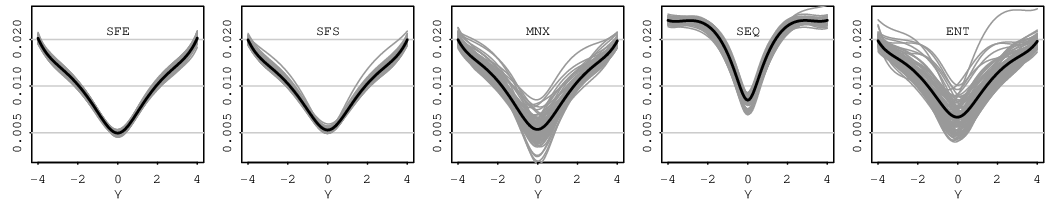
Refer to caption
Figure 4: Relative standard error plots based on 100 replications of the autologistic model with κ=0.5\kappa=0.5 fixed and γ\gamma varying. The bold line provides the average of the relative standard errors.

S10 Analysis of radionuclide concentrations using spatial GLMM

The dataset consists of spatial measurements of γ\gamma-ray counts yiy_{i} observed during ℓi\ell_{i} seconds at the iith coordinate on the Rongelap island, i=1,…,157i=1,\ldots,157. These data were analyzed by Diggle et al., (1998) and Evangelou and Roy, (2019) among others using a spatial generalized linear mixed model (SGLMM). We consider a Poisson SGLMM using a parametric link function for the γ\gamma-ray counts, that is, we assume yi|μi∼indPo⁡(ℓi​μi)y_{i}|\mu_{i}\mathrel{\mathop{\kern 0.0pt\sim}\limits^{\text{ind}}}\mathrm{Po}(\ell_{i}\mu_{i}) with gλ​(μi)=zig_{\lambda}(\mu_{i})=z_{i} for i=1,…,157,i=1,\dots,157, where gλ​(⋅)g_{\lambda}(\cdot) is a modified Box-Cox link given in Evangelou and Roy, (2019) with parameter λ\lambda, and ziz_{i}’s are the latent variables. Let 𝒚\boldsymbol{y} and 𝝁\boldsymbol{\mu} denote the vectors of yiy_{i}’s and μi\mu_{i}’s, respectively. Then 𝒛=(z1,…,z157)\boldsymbol{z}=(z_{1},\dots,z_{157}) is modeled by a multivariate Gaussian distribution corresponding to a Gaussian random field (GRF) 𝒵\mathcal{Z} at the sampled locations. In particular, we assume 𝒵|β,σ2∼GRF⁡(β,σ2,ϕ,ω,κ)\mathcal{Z}|\beta,\sigma^{2}\sim\mathrm{GRF}(\beta,\sigma^{2},\phi,\omega,\kappa), the GRF with constant mean β\beta, Matérn correlation, variance σ2\sigma^{2}, range ϕ\phi, relative nugget ω\omega and smoothness κ\kappa. The partial sill parameter σ2\sigma^{2} is assigned a scaled-inverse-chi-square prior (ScInv​𝒳2​(1,1)\mathrm{ScInv}\mathcal{X}^{2}(1,1)), and conditioned on σ2\sigma^{2}, the mean parameter β∼N⁡(0,100​σ2)\beta\sim N(0,100\sigma^{2}). Let ξ=(λ,ϕ,ω,κ)\xi=(\lambda,\phi,\omega,\kappa). We consider estimating the marginal likelihood for ξ\xi (relative to an arbitrary reference point ξ1=ξ~\xi_{1}=\tilde{\xi} to be defined later) by (1.2) in the main paper. Note that, the empirical Bayes estimate of ξ\xi is the point where the marginal likelihood function is maximized (Roy et al.,, 2016, see e.g.). Since β,σ2\beta,\sigma^{2} can be analytically integrated out, one can work with the posterior density of 𝒛\boldsymbol{z}, πξ​(𝒛|𝒚)\pi_{\xi}(\boldsymbol{z}|\boldsymbol{y}). Here, we consider multiple IS estimator (1.2) in the main paper based on samples from the (transformed) density πξ​(𝝁|𝒚)\pi_{\xi}(\boldsymbol{\mu}|\boldsymbol{y}) (see Evangelou and Roy,, 2019, for the reasons for considering the transformed samples). Thus, here Q=Π={πξ​(𝝁|𝒚),ξ∈Ξ}Q=\Pi=\{\pi_{\xi}(\boldsymbol{\mu}|\boldsymbol{y}),\xi\in\Xi\} for some Ξ\Xi defined later.

In order to narrow down the potential region of search, we initially choose a wide range of values for each component of ξ\xi, and form a large grid, denoted by Ξ\Xi, by combining discrete points within these ranges. This gives us the set consisting of the following 949^{4} points:

Ξ={0,0.5,…,4}×{100,425,…,2700}×{0,0.75,…,6}×{0.1,0.35,…,2.1}.\Xi=\{0,0.5,\ldots,4\}\times\{100,425,\ldots,2700\}\times\{0,0.75,\ldots,6\}\times\{0.1,0.35,\ldots,2.1\}.

The SFE method, after each range is scaled in [0,1][0,1], was applied to choose k=5k=5 points from Ξ\Xi. Markov chain samples from the kk densities πξi​(𝝁|𝒚),i=1,…,k\pi_{\xi_{i}}(\boldsymbol{\mu}|\boldsymbol{y}),i=1,\dots,k corresponding to this preliminary skeleton set are generated. We evaluate (1.2) in the main paper with Nl=1000,nl=1000,l=1,…,5N_{l}=1000,n_{l}=1000,l=1,\dots,5 for all points in Ξ\Xi, and retain only those points for which the value of (1.2) in the main paper is not less than 60% of the maximum value. The maximum value is attained at ξ~=(1,425,2.25,0.6)\tilde{\xi}=(1,425,2.25,0.6) and there are 33 points satisfying this criterion. These points form the search set Ξ~\tilde{\Xi} which is a subset of

Ξ~⊂{1}×{100,425,…,1400}×{1.50,2.25,…,4.50}×{0.35,0.60,…,2.10}.\tilde{\Xi}\subset\{1\}\times\{100,425,\ldots,1400\}\times\{1.50,2.25,\ldots,4.50\}\times\{0.35,0.60,\ldots,2.10\}.

Our aim is to choose k=5k=5 elements from Ξ~\tilde{\Xi}, one of which must be ξ~\tilde{\xi}, to form the skeleton sets, using the methods discussed in Section 3 of the main paper, with the objective of estimating the ratios of marginal densities in Ξ\Xi relative to ξ~\tilde{\xi}. The naive IS method with samples from the posterior density πξ~​(𝝁|𝒚)\pi_{\tilde{\xi}}(\boldsymbol{\mu}|\boldsymbol{y}) is considered for comparison.

The SFE optimal set is computed on Ξ~\tilde{\Xi} after each dimension is scaled in [0,1][0,1]. For SFS, we write (3.7b) in the main paper as an integral over (𝒛,log⁡σ2)(\boldsymbol{z},\log\sigma^{2}), because the prior for 𝒛\boldsymbol{z} is multivariate normal and σ2>0\sigma^{2}>0, and use the approximation given in Section S1 of the supplementary materials. The SEQ, MNX, and ENT optimal sets are computed iteratively. At each iteration, an estimate of the asymptotic relative standard error is computed using Theorem 2(a) based on 1000 samples for the first stage and 1000 samples for the second stage. We use different empirical convergence diagnostics (Roy,, 2020) to check mixing of the Markov chains. Further computational details about our implementation are provided in Section S10.1 of this supplementary materials.

Finally, for each obtained skeleton set, we generate new samples which we use to estimate the ratio of the marginal likelihoods and its relative standard error for all ξ∈Ξ\xi\in\Xi. We generate a total of 50,000 samples which are equally divided between each proposal density (see Section S10.1 for further details). The maximum relative standard error estimates corresponding to one component of ξ\xi fixed across the other components are shown in Figure 5. It can be seen that across all parameters, naive IS and SEQ have the highest variance, and that SFS, MNX, ENT have the lowest maximum variance.

Refer to caption
Figure 5: Profile relative standard errors estimates for the Rongelap data. One parameter is fixed and the maximum relative standard error across the other parameters is plotted against the fixed parameter. The crosses indicate points included in the skeleton set.

S10.1 Computational details

Here we give more details on how we produced the results in this Section. The computation is done in two phases. In the first phase we find the optimal skeleton set, 𝝃{\boldsymbol{\xi}}, for each method. In the second phase we compare the relative standard error of the naive and multiple IS estimators using the skeleton sets computed in the first phase. The total number of samples used for each method in the second phase is kept fixed and the same. In all calculations involving the asymptotic variance of the IS estimator, the SV estimate with the Tukey-Hanning window,

wn​(j)=0.5​[1+cos⁡(π​|j|/bn)]​I​(|j|<bn),w_{n}(j)=0.5[1+\cos(\pi|j|/b_{n})]I(|j|<b_{n}),

was used, where bn=nb_{n}=\sqrt{n}. Markov chain samples are generated using the algorithm of Diggle et al., (1998).

Phase 1: Finding the optimal set of proposal densities

  • •

    NIS: This is not required because the proposal density is fixed at 𝝃nis={ξ~}={(1,425,2.25,0.6)}{\boldsymbol{\xi}}_{\mathrm{nis}}=\{\tilde{\xi}\}=\{(1,425,2.25,0.6)\}.

  • •

    SFE: This method is based on the Euclidean distance between the parameters. Each component of the parameter set Ξ~\tilde{\Xi} is scaled to vary between 0 and 1 before the optimal set is computed. The point-swapping algorithm of Section S7.1 is used to find the optimal set. We find
    𝝃sfe={ξ~,(1,100,3,1.85),(1,425,3.75,0.6),(1,750,3,0.35),(1,1075,1.5,0.35)}{\boldsymbol{\xi}}_{\mathrm{sfe}}=\{\tilde{\xi},(1,100,3,1.85),(1,425,3.75,0.6),(1,750,3,0.35),(1,1075,1.5,0.35)\}.

  • •

    SFS: This method requires the SKLD between two densities corresponding to two values of ξ\xi. We first write the integrals in (3.7a) of the main paper in terms of (𝒛,log⁡σ2)(\boldsymbol{z},\log\sigma^{2}), because the prior for 𝒛\boldsymbol{z} is multivariate normal and σ2>0\sigma^{2}>0. Each ratio of integrals is approximated using the Laplace’s method given in Section S1. The point-swapping algorithm of Section S7.1 is used to find the optimal set. We find
    𝝃sfs={ξ~,(1,425,3,0.6),(1,425,3.75,1.1),(1,425,4.5,0.6),(1,750,1.5,0.35)}{\boldsymbol{\xi}}_{\mathrm{sfs}}=\{\tilde{\xi},(1,425,3,0.6),(1,425,3.75,1.1),(1,425,4.5,0.6),(1,750,1.5,0.35)\}.

  • •

    SEQ: In this case the optimal set is computed by starting at 𝝃(1)=𝝃nis{\boldsymbol{\xi}}^{(1)}={\boldsymbol{\xi}}_{\mathrm{nis}}. Then, given that at the iith iteration, i=2,…,ki=2,\ldots,k we are at 𝝃(i−1){\boldsymbol{\xi}}^{(i-1)}, we obtain 𝝃(i)=𝝃(i−1)∪{ξ′}{\boldsymbol{\xi}}^{(i)}={\boldsymbol{\xi}}^{(i-1)}\cup\{\xi^{\prime}\}, where ξ′\xi^{\prime} corresponds to the point in Ξ~∖𝝃(i−1)\tilde{\Xi}\setminus{\boldsymbol{\xi}}^{(i-1)} with the highest relative standard error. The relative standard error is again computed using 1,000 Gibbs samples for stage 1 and 1,000 new samples for stage 2. We find
    𝝃seq={ξ~,(1,100,2.25,1.35),(1,100,2.25,1.6),(1,425,3,1.1),(1,425,3.75,1.1)}{\boldsymbol{\xi}}_{\mathrm{seq}}=\{\tilde{\xi},(1,100,2.25,1.35),(1,100,2.25,1.6),(1,425,3,1.1),(1,425,3.75,1.1)\}.

  • •

    MNX: The optimal set is found by simulated annealing (Section S7.2). We start the simulated annealing algorithm at 𝝃sfs{\boldsymbol{\xi}}_{\mathrm{sfs}} and perform imax=250i_{\mathrm{max}}=250 iterations with T0=0.001T_{0}=0.001 and B=10B=10. The SV estimates were calculated using 1,000 Gibbs samples for stage 1 and 1,000 new samples for stage 2. We find
    𝝃mnx={ξ~,(1,100,2.25,1.85),(1,425,1.5,0.6),(1,425,2.25,1.1),(1,1075,3,0.35)}{\boldsymbol{\xi}}_{\mathrm{mnx}}=\{\tilde{\xi},(1,100,2.25,1.85),(1,425,1.5,0.6),(1,425,2.25,1.1),(1,1075,3,0.35)\}.

  • •

    ENT: The optimal set is found by simulated annealing (Section S7.2). We start the simulated annealing algorithm at 𝝃sfs{\boldsymbol{\xi}}_{\mathrm{sfs}} and perform imax=250i_{\mathrm{max}}=250 iterations with T0=10T_{0}=10 and B=10B=10. The optimality criterion used for this method is −log⁡det​(U)-\log\mbox{det}(U) where UU is the matrix with (i,j)(i,j)th element Ui​j=(V^𝒒)i​j/(d^i​d^j)U_{ij}=(\widehat{V}_{\boldsymbol{q}})_{ij}/(\hat{d}_{i}\hat{d}_{j}). The estimates 𝒅^\hat{\boldsymbol{d}} and V^𝒒\widehat{V}_{\boldsymbol{q}} are computed from 1,000 Gibbs samples. We find
    𝝃ent={ξ~,(1,100,2.25,1.35),(1,425,3,1.1),(1,750,3.75,0.35),(1,1075,1.5,0.35)}{\boldsymbol{\xi}}_{\mathrm{ent}}=\{\tilde{\xi},(1,100,2.25,1.35),(1,425,3,1.1),(1,750,3.75,0.35),(1,1075,1.5,0.35)\}.

Phase 2: Estimation of the ratio of marginal densities

After the skeleton sets are found, we generate a total of M=50,000M=\text{50,000} samples from the proposal densities, equally divided among all densities in the set. Thus, for NIS we simply take MM samples from the density corresponding to 𝝃nis{\boldsymbol{\xi}}_{\mathrm{nis}} and for the multiple IS methods we take M/kM/k samples from each density in the corresponding 𝝃{\boldsymbol{\xi}} set. However, the total of M/kM/k samples must be split into stage 1, for estimating the ratio of marginals within 𝝃{\boldsymbol{\xi}}, 𝒅\boldsymbol{d}, and stage 2, for estimating the ratio of marginals over the whole set Ξ\Xi. To determine the optimal split we use equation (S8.15) where υ^1​(ξ)\hat{\upsilon}_{1}(\xi) and υ^2​(ξ)\hat{\upsilon}_{2}(\xi) are calculated from 1,000 stage 1 and 1,000 stage 2 samples. For MNX, SEQ, and ENT the existing samples from Phase 1 are reused but for the space-filling methods, new samples are generated. We take N^/k\hat{N}/k stage 1 samples from each density in the skeleton set where N^\hat{N} is the integer that minimizes maxξ∈Ξ⁡RelSE⁡(ξ,N,M−N)\max_{\xi\in\Xi}\mathrm{RelSE}(\xi,N,M-N), and n^/k\hat{n}/k stage 2 samples, where n^=M−N^\hat{n}=M-\hat{N}. This corresponds to stage 1 sample sizes of 500 and stage 2 sample sizes of 9,500 from each density for all methods.

References

  • Bélisle, (1992) Bélisle, C. J. (1992). Convergence theorems for a class of simulated annealing algorithms on RdR^{d}. J. App. Prob., 29(4):885–895.
  • Besag, (1974) Besag, J. (1974). Spatial interaction and the statistical analysis of lattice systems. J. Royal Statist. Soc., Ser. B, 36(2):192–225.
  • Borchers, (2021) Borchers, H. W. (2021). pracma: Practical Numerical Math Functions. R package version 2.3.3.
  • Buta and Doss, (2011) Buta, E. and Doss, H. (2011). Computational approaches for empirical Bayes methods and Bayesian sensitivity analysis. Ann. Statist., 39:2658–2685.
  • Cappé et al., (2004) Cappé, O., Guillin, A., Marin, J. M., and Robert, C. P. (2004). Population Monte Carlo. J. Comp. and Graph. Statist., 13:907–929.
  • Christensen, (2004) Christensen, O. F. (2004). Monte Carlo maximum likelihood in model-based geostatistics. J. Comp. and Graph. Statist., 13(3):702–718.
  • Diggle et al., (1998) Diggle, P. J., Tawn, J. A., and Moyeed, R. A. (1998). Model-based geostatistics. J. Royal Statist. Soc.: Ser. C (Applied Statist.), 47(3):299–350.
  • Doss, (2010) Doss, H. (2010). Estimation of large families of Bayes factors from Markov chain output. Statist. Sinica, 20:537–560.
  • Doss and Tan, (2014) Doss, H. and Tan, A. (2014). Estimates and standard errors for ratios of normalizing constants. J. Royal Statist. Soc., Ser. B, 76:683–712.
  • Elvira et al., (2019) Elvira, V., Martino, L., Luengo, D., and Bugallo, M. F. (2019). Generalized multiple importance sampling. Statist. Sci., 34(1):129–155.
  • Evangelou and Roy, (2019) Evangelou, E. and Roy, V. (2019). Estimation and prediction for spatial generalized linear mixed models with parametric links via reparameterized importance sampling. Spatial Statist., 29:289–315.
  • Evangelou and Roy, (2022) Evangelou, E. and Roy, V. (2022). geoBayes: Analysis of Geostatistical Data using Bayes and Empirical Bayes Methods. R package version 0.7.1.
  • Evangelou et al., (2011) Evangelou, E., Zhu, Z., and Smith, R. L. (2011). Estimation and prediction for spatial generalized linear mixed models using high order Laplace approximation. J. Statist. Plan. and Infer., 141(11):3564–3577.
  • Fang et al., (2006) Fang, K.-T., Li, R., and Sudjianto, A. (2006). Design and Modeling for Computer Experiments. Chapman & Hall/CRC.
  • Finney, (1947) Finney, D. J. (1947). The estimation from individual records of the relationship between dose and quantal response. Biometrika, 34:320–334.
  • Flegal and Jones, (2010) Flegal, J. M. and Jones, G. L. (2010). Batch means and spectral variance estimators in Markov chain Monte Carlo. Ann. Statist., 38:1034–1070.
  • George and Doss, (2018) George, C. P. and Doss, H. (2018). Principled selection of hyperparameters in the latent Dirichlet allocation model. J. Machine Learn. Res., 18(162):1–38.
  • Geyer, (1994) Geyer, C. J. (1994). Estimating normalizing constants and reweighting mixtures in Markov chain Monte Carlo. Technical Report 568, School of Statistics, University of Minnesota.
  • Geyer, (2011) Geyer, C. J. (2011). Handbook of Markov chain Monte Carlo, chapter Importance Sampling, Simulated Tempering, and Umbrella Sampling, pages 295–311. CRC Press, Boca Raton, FL.
  • Geyer and Thompson, (1992) Geyer, C. J. and Thompson, E. A. (1992). Constrained Monte Carlo maximum likelihood for dependent data. J. Royal Statist. Soc., Ser. B, 54:657–699.
  • Geyer and Thompson, (1995) Geyer, C. J. and Thompson, E. A. (1995). Annealing Markov chain Monte Carlo with applications to ancestral inference. J. Amer. Statist. Assoc., 90:909–920.
  • Ghosh et al., (2007) Ghosh, J. K., Delampady, M., and Samanta, T. (2007). An introduction to Bayesian analysis: theory and methods. Springer Science & Business Media.
  • Gill et al., (1988) Gill, R. D., Vardi, Y., and Wellner, J. A. (1988). Large sample theory of empirical distributions in biased sampling models. Ann. Statist., 16:1069–1112.
  • Kaiser et al., (2012) Kaiser, M. S., Caragea, P. C., and Furukawa, K. (2012). Centered parameterizations and dependence limitations in Markov random field models. J. Statist. Plan. and Infer., 142(7):1855–1863.
  • Kaiser and Cressie, (2000) Kaiser, M. S. and Cressie, N. (2000). The construction of multivariate distributions from Markov random fields. J. Mult. Analysis, 73(2):199–220.
  • Kass, (1989) Kass, R. E. (1989). The geometry of asymptotic inference. Statist. Sci., pages 188–219.
  • Ko et al., (1995) Ko, C.-W., Lee, J., and Queyranne, M. (1995). An exact algorithm for maximum entropy sampling. Oper. Res., 43(4):684–691.
  • Kong et al., (2003) Kong, A., McCullagh, P., Meng, X.-L., Nicolae, D., and Tan, Z. (2003). A theory of statistical models for Monte Carlo integration (with discussion). J. Royal Statist. Soc., Ser. B, 65:585–618.
  • Li et al., (2013) Li, W., Tan, Z., and Chen, R. (2013). Two-stage importance sampling with mixture proposals. J. Amer. Statist. Assoc., 108(504):1350–1365.
  • Marinari and Parisi, (1992) Marinari, E. and Parisi, G. (1992). Simulated tempering: A new Monte Carlo scheme. Europhy. Lett., 19:451–458.
  • Meng and Wong, (1996) Meng, X.-L. and Wong, W. H. (1996). Simulating ratios of normalizing constants via a simple identity: A theoretical exploration. Statist. Sinica, 6:831–860.
  • Nychka et al., (2017) Nychka, D., Furrer, R., Paige, J., and Sain, S. (2017). fields. R package version 9.0.
  • Owen and Zhou, (2000) Owen, A. and Zhou, Y. (2000). Safe and effective importance sampling. J. Amer. Statist. Assoc., 95:135–143.
  • Rao, (1982) Rao, C. R. (1982). Diversity: Its measurement, decomposition, apportionment and analysis. Sankhyā: The Ind. J. Statist., Ser. A, pages 1–22.
  • Roy, (2014) Roy, V. (2014). Efficient estimation of the link function parameter in a robust Bayesian binary regression model. Comp. Statist. and Data Ana., 73:87–102.
  • Roy, (2020) Roy, V. (2020). Convergence diagnostics for Markov chain Monte Carlo. Ann. Rev. Statist. and Its App., 7:387–412.
  • Roy and Chakraborty, (2017) Roy, V. and Chakraborty, S. (2017). Selection of tuning parameters, solution paths and standard errors for Bayesian lassos. Bayes. Anal., 12:753–778.
  • Roy et al., (2016) Roy, V., Evangelou, E., and Zhu, Z. (2016). Efficient estimation and prediction for the Bayesian binary spatial model with flexible link functions. Biometrics, 72:289–298.
  • Roy et al., (2018) Roy, V., Tan, A., and Flegal, J. (2018). Estimating standard errors for importance sampling estimators with multiple Markov chains. Statist. Sinica, 28:1079–1101.
  • Royle and Nychka, (1998) Royle, J. A. and Nychka, D. (1998). An algorithm for the construction of spatial coverage designs with implementation in SPLUS. Computers & Geosciences, 24(5):479–488.
  • Sherman et al., (2006) Sherman, M., Apanasovich, T. V., and Carroll, R. J. (2006). On estimation in binary autologistic spatial models. J. Statist. Comp. and Simu., 76(2):167–179.
  • Shewry and Wynn, (1987) Shewry, M. C. and Wynn, H. P. (1987). Maximum entropy sampling. J. Appl. Statist., 14(2):165–170.
  • Stan Development Team, (2020) Stan Development Team (2020). RStan: the R interface to Stan. R package version 2.21.2.
  • Tan et al., (2015) Tan, A., Doss, H., and Hobert, J. P. (2015). Honest importance sampling with multiple Markov chains. J. Comp. and Graph. Statist., 24:792–826.
  • Tan, (2004) Tan, Z. (2004). On a likelihood approach for Monte Carlo integration. J. Amer. Statist. Assoc., 99:1027–1036.
  • Vardi, (1985) Vardi, Y. (1985). Empirical distributions in selection bias models. Ann. Statist., 13:178–203.
  • Vats et al., (2018) Vats, D., Flegal, J. M., and Jones, G. L. (2018). Strong consistency of the multivariate spectral variance estimator in Markov chain Monte Carlo. Bernoulli, 24:1860–1909.
  • Veach and Guibas, (1995) Veach, E. and Guibas, L. (1995). Optimally combining sampling techniques for Monte Carlo rendering. SIGGRAPH 95 Conference Proceedings, Reading MA. Addison-Wesley, pages 419–428.