跳到论文正文
W Papers独立论文阅读器 arXiv:1805.00693 论文正文 计算阅读时间 · 0%
引用这篇论文根据当前论文元数据生成,正式投稿前建议核对。


License: arXiv.org perpetual non-exclusive license
arXiv:1805.00693v1 [math.NA] 02 May 2018

A Cut Finite Element Method for Elliptic Bulk Problems with Embedded Surfaces

Erik Burman     Peter Hansbo     Mats G. Larson     David Samvin
Abstract

We propose an unfitted finite element method for flow in fractured porous media. The coupling across the fracture uses a Nitsche type mortaring, allowing for an accurate representation of the jump in the normal component of the gradient of the discrete solution across the fracture. The flow field in the fracture is modelled simultaneously, using the average of traces of the bulk variables on the fractured. In particular the Laplace-Beltrami operator for the transport in the fracture is included using the average of the projection on the tangential plane of the fracture of the trace of the bulk gradient. Optimal order error estimates are proven under suitable regularity assumptions on the domain geometry. The extension to the case of bifurcating fractures is discussed. Finally the theory is illustrated by a series of numerical examples.

1 Introduction

We consider a model Darcy creeping flow problem with low permeability in the bulk and with embedded interfaces with high permeability. Our approach is based on the Nitsche extended finite element of Hansbo and Hansbo [12], which however did not include transport on the interface. Here, we follow Capatina et al. [6] and let a suitable mean of the solution on the interface be affected by a transport equation see also [2]. We present a complete a priori analysis and consider the important extension to bifurcating fractures.

The flow model we use is essentially the one proposed in [6]. More sophisticated models have been proposed, e.g., in [1, 9, 10, 14], in particular allowing for jumps in the solution across the interfaces. To allow for such jumps, one can either align the mesh with the interfaces, as in, e.g., [11], or use extended finite element techniques, cf. [2, 6, 7, 8].

In previous work [4] we used a continuous approximation with the interface equations simply added to the bulk equation, which does not allow for jumps in the solution. This paper presents a more complex but more accurate discrete solution to the problem. To reduce the technical detail of the arguments we consider a semi-discretization of the problem where we assume that the integrals on the interface and the subdomains separated by the interface can be evaluated exactly. The results herein can be extended to the fully discrete setting, with a piecewise affine approximation of the fracture using the analysis detailed in [5].

An outline of the paper is as follows: In Section 2 we formulate the model problem, its weak form, and investigate the regularity properties of the solution, in Section 3 we formulate the finite element method, in Section 4 we derive error estimates, in Section 5 we extend the approach to the case of bifurcating fractures, and in Section 6 we present numerical examples including a study of the convergence and a more applied example with a network of fractures.

2 The Model Problem

In this section we introduce our modelproblem. First we present the strong form of the equations and then we derive the weak form that is used for the finite element modelling. We discuss the regularity properties of the solution and show that if the fracture is sufficiently smooth the problem solution, restricted to the subdomains partitioning the global domain, has a regularity that allows for optimal approximation estimates for piecewise affine finite element methods.

2.1 Strong and Weak Formulations

Let Ω\Omega be a convex polygonal domain in ℝd\mathbb{R}^{d}, with d=2d=2 or 33. Let Γ\Gamma be a smooth embedded interface in Ω\Omega, which partitions Ω\Omega into two subdomains Ω1\Omega_{1} and Ω2\Omega_{2}. We consider the problem: find u:Ω→ℝu:\Omega\rightarrow\mathbb{R} such that

−∇⋅a∇u\displaystyle-\nabla\cdot a\nabla u =f\displaystyle=f in Ωi\Omega_{i}, i=1,2i=1,2 (2.1)
−∇Γ⋅aΓ∇ΓuΓ\displaystyle-\nabla_{\Gamma}\cdot a_{\Gamma}\nabla_{\Gamma}u_{\Gamma} =fΓ−⟦n⋅a∇u⟧\displaystyle=f_{\Gamma}-\llbracket n\cdot a\nabla u\rrbracket on Γ\Gamma (2.2)
[u]\displaystyle[u] =0\displaystyle=0 on Γ\Gamma (2.3)
u\displaystyle u =0\displaystyle=0 on ∂Ω\partial\Omega (2.4)

Here

[v]=v1−v2,⟦n⋅a∇v⟧=n1⋅a1∇v1+n2⋅a2∇v2[v]=v_{1}-v_{2},\hskip 20.00003pt\llbracket n\cdot a\nabla v\rrbracket=n_{1}\cdot a_{1}\nabla v_{1}+n_{2}\cdot a_{2}\nabla v_{2} (2.5)

where vi=v|H1​(Ωi)v_{i}=v|_{H^{1}(\Omega_{i})}, nin_{i} is the exterior unit normal to Ωi\Omega_{i}, aia_{i} are positive bounded permeability coefficients, for simplicity taken as constant, and 0≤aΓ<∞0\leq a_{\Gamma}<\infty is a constant permeability coefficient on the interface. Note that it follows from (2.3) that vv is continuous across Γ\Gamma while from (2.3) we conclude that the normal flux is in general not continuous across Γ\Gamma. Note also that taking aΓ=0a_{\Gamma}=0 and fΓ=0f_{\Gamma}=0 corresponds to a standard Poisson problem with possible jump in permeability coefficient across Γ\Gamma.

Refer to caption
Figure 1: Schematic figure of bifurcating fractures.

To derive the weak formulation of the system we introduce the L2L^{2}-scalar product over a domain X⊂ℝdX\subset\mathbb{R}^{d}, or X⊂ℝd−1X\subset\mathbb{R}^{d-1}. For u,v∈L2​(X)u,v\in L^{2}(X) let

(u,v)X=∫Xu​v​d​X(u,v)_{X}=\int_{X}u\,v~\mbox{d}X (2.6)

with the associated norm ‖u‖X=(u,u)X1/2\|u\|_{X}=(u,u)_{X}^{1/2}. Multiplying (2.1) by v∈V=H1​(Ω)∩H1​(Γ)v\in V=H^{1}(\Omega)\cap H^{1}(\Gamma), integrating by parts over Ωi\Omega_{i}, and using (2.2) we obtain

(f,v)Ω\displaystyle(f,v)_{\Omega} =−(∇⋅a∇u,v)Ω1−(∇⋅a∇u,v)Ω2\displaystyle=-(\nabla\cdot a\nabla u,v)_{\Omega_{1}}-(\nabla\cdot a\nabla u,v)_{\Omega_{2}} (2.7)
=(a∇u,∇v)Ω1+(a∇u,∇v)Ω2−(⟦n⋅a∇u⟧,v)Γ\displaystyle=(a\nabla u,\nabla v)_{\Omega_{1}}+(a\nabla u,\nabla v)_{\Omega_{2}}-(\llbracket n\cdot a\nabla u\rrbracket,v)_{\Gamma} (2.8)
=(a∇u,∇v)Ω−(fΓ+∇Γ⋅aΓ∇Γu,v)Γ\displaystyle=(a\nabla u,\nabla v)_{\Omega}-(f_{\Gamma}+\nabla_{\Gamma}\cdot a_{\Gamma}\nabla_{\Gamma}u,v)_{\Gamma} (2.9)
=(a∇u,∇v)Ω+(aΓ∇Γu,∇Γv)Γ−(fΓ,v)Γ\displaystyle=(a\nabla u,\nabla v)_{\Omega}+(a_{\Gamma}\nabla_{\Gamma}u,\nabla_{\Gamma}v)_{\Gamma}-(f_{\Gamma},v)_{\Gamma} (2.10)

We thus arrive at the weak formulation: find u∈Vu\in V such that

(a∇u,∇v)Ω+(aΓ∇Γu,∇Γv)Γ=(f,v)Ω+(fΓ,v)Γ∀v∈V(a\nabla u,\nabla v)_{\Omega}+(a_{\Gamma}\nabla_{\Gamma}u,\nabla_{\Gamma}v)_{\Gamma}=(f,v)_{\Omega}+(f_{\Gamma},v)_{\Gamma}\hskip 20.00003pt\forall v\in V (2.11)

Observing that VV is a Hilbert space with scalar product

a(v,w)=(a∇v,∇w)Ω+(aΓ∇Γv,∇Γw)Γa(v,w)=(a\nabla v,\nabla w)_{\Omega}+(a_{\Gamma}\nabla_{\Gamma}v,\nabla_{\Gamma}w)_{\Gamma} (2.12)

and associated norm ‖v‖a2=a⁡(v,v)\|v\|^{2}_{a}=a(v,v) it follows from the Lax-Milgram Lemma that there is a unique solution to (2.11) in VV for f∈H−1​(Ω)f\in H^{-1}(\Omega) and fΓ∈H−1​(Γ)f_{\Gamma}\in H^{-1}(\Gamma).

2.2 Regularity Properties

To prove optimality of our finite element method we need that the exact solution is sufficient is sufficiently regular. However since the normal fluxes jumps over the interface the solution can not have square integrable weak second derivatives. If the interface is smooth however we will prove that the solution restricted to the different subdomains Ω1\Omega_{1}, Ω2\Omega_{2} and Γ\Gamma is regular. The upshot of the unfitted finite element is that this local regularity is sufficient for optimal order approximation. More precisely we have the elliptic regularity estimate

‖u‖H2​(Ω1)+‖u‖H2​(Ω2)+‖u‖H2​(Γ)≲‖f‖Ω+‖fΓ‖Γ\|u\|_{H^{2}(\Omega_{1})}+\|u\|_{H^{2}(\Omega_{2})}+\|u\|_{H^{2}(\Gamma)}\lesssim\|f\|_{\Omega}+\|f_{\Gamma}\|_{\Gamma} (2.13)

Proof.Let ui∈H01​(Ωi)u_{i}\in H^{1}_{0}(\Omega_{i}) solve

(ai∇ui,∇v)Ωi=(f,v)Ωi∀v∈H01(Ωi)(a_{i}\nabla u_{i},\nabla v)_{\Omega_{i}}=(f,v)_{\Omega_{i}}\hskip 20.00003pt\forall v\in H^{1}_{0}(\Omega_{i}) (2.14)

Then we have

‖ui‖H2​(Ωi)≲‖f‖Ωii=1,2\|u_{i}\|_{H^{2}(\Omega_{i})}\lesssim\|f\|_{\Omega_{i}}\hskip 20.00003pti=1,2 (2.15)

Writing u=uΓ+u1+u2u=u_{\Gamma}+u_{1}+u_{2} where uΓu_{\Gamma} satisfies

−∇Γ⋅aΓ∇ΓuΓ\displaystyle-\nabla_{\Gamma}\cdot a_{\Gamma}\nabla_{\Gamma}u_{\Gamma} =fΓ+⟦n⋅a∇(uΓ+u1+u2)⟧\displaystyle=f_{\Gamma}+\llbracket n\cdot a\nabla(u_{\Gamma}+u_{1}+u_{2})\rrbracket (2.16)
=fΓ+⟦n⋅a∇uΓ⟧+n1⋅a∇u1+n2⋅a∇u2on Γ\displaystyle=f_{\Gamma}+\llbracket n\cdot a\nabla u_{\Gamma}\rrbracket+n_{1}\cdot a\nabla u_{1}+n_{2}\cdot a\nabla u_{2}\hskip 20.00003pt\text{on $\Gamma$} (2.17)

and

−∇⋅a∇uΓ=0on Ωi, i=1,2-\nabla\cdot a\nabla u_{\Gamma}=0\hskip 20.00003pt\text{on $\Omega_{i}$, $i=1,2$} (2.18)

Using (2.15) we conclude that

ni⋅a∇ui|Γ∈H1/2(Γ)i=1,2n_{i}\cdot a\nabla u_{i}|_{\Gamma}\in H^{1/2}(\Gamma)\hskip 20.00003pti=1,2 (2.19)

Furthermore, using that uΓ∈H1​(Γ)u_{\Gamma}\in H^{1}(\Gamma), which follows from the fact that uΓ∈Vu_{\Gamma}\in V it follows that uΓ|Ωi∈H3/2​(Ωi)u_{\Gamma}|_{\Omega_{i}}\in H^{3/2}(\Omega_{i}), i=1,2,i=1,2, and thus

⟦n⋅a∇uΓ⟧∈H1/2(Γ)\llbracket n\cdot a\nabla u_{\Gamma}\rrbracket\in H^{1/2}(\Gamma) (2.20)

Since the right hand side of (2.17) is in L2​(Γ)L^{2}(\Gamma) we may use elliptic regularity for the Laplace Beltrami operator to confirm that

uΓ|Γ∈H2​(Γ)u_{\Gamma}|_{\Gamma}\in H^{2}(\Gamma) (2.21)

Collecting the bounds we obtain the refined regularity estimate

‖uΓ‖H2​(Γ)+∑i=12(‖uΓ‖H5/2​(Ωi)+‖ui‖H2​(Ωi))≲‖f‖Ω+‖fΓ‖Γ\|u_{\Gamma}\|_{H^{2}(\Gamma)}+\sum_{i=1}^{2}\left(\|u_{\Gamma}\|_{H^{5/2}(\Omega_{i})}+\|u_{i}\|_{H^{2}(\Omega_{i})}\right)\lesssim\|f\|_{\Omega}+\|f_{\Gamma}\|_{\Gamma} (2.22)

where we note that we have stronger control of uΓu_{\Gamma} on the subdomains. ∎

3 The Finite Element Method

3.1 The Mesh and Finite Element Space

Let 𝒯h\mathcal{T}_{h} be a quasi uniform conforming mesh, consisting of shape regular elements with mesh parameter h∈(0,h0]h\in(0,h_{0}], on Ω\Omega and let

𝒯h,i={T∈𝒯h:T∩Ωi≠∅}i=1,2\mathcal{T}_{h,i}=\{T\in\mathcal{T}_{h}:T\cap\Omega_{i}\neq\emptyset\}\hskip 20.00003pti=1,2 (3.1)

be the active meshes associated with Ωi\Omega_{i}, i=1,2.i=1,2. Let VhV_{h} be a finite element space consisting of continuous piecewise polynomials on 𝒯h\mathcal{T}_{h} and define

Vh,i=Vh|𝒯hii=1,2V_{h,i}=V_{h}|_{\mathcal{T}_{h_{i}}}\hskip 20.00003pti=1,2 (3.2)

and

Wh=Vh,1⊕Vh,2W_{h}=V_{h,1}\oplus V_{h,2} (3.3)

To v=v1⊕v2∈Whv=v_{1}\oplus v_{2}\in W_{h} we associate the function v~∈L2​(Ω)\widetilde{v}\in L^{2}(\Omega) such that v~|Ωi=vi|Ωi\widetilde{v}|_{\Omega_{i}}=v_{i}|_{\Omega_{i}}, i=1,2i=1,2. In general, we simplify the notation and write v~=v\widetilde{v}=v.

3.2 Derivation of the Method

To derive the finite element method we follow the same approach as when introducing the weak formulation, but taking care to handle the boundary integrals that appear due to the discontinuities in the approximation space.

Testing the exact problem with v∈Whv\in W_{h} and integrating by parts over Ω1\Omega_{1} and Ω2\Omega_{2} we find that

(f,v)Ω1+(f,v)Ω2\displaystyle(f,v)_{\Omega_{1}}+(f,v)_{\Omega_{2}} (3.4)
=(−∇⋅a∇u,v)Ω1+(−∇⋅a∇u,v)Ω2\displaystyle\hskip 20.00003pt=(-\nabla\cdot a\nabla u,v)_{\Omega_{1}}+(-\nabla\cdot a\nabla u,v)_{\Omega_{2}} (3.5)
=(a∇u,∇v)Ω−(⟨n⋅a∇u⟩,[v])Γ−(⟦n⋅a∇u⟧,⟨v⟩∗)Γ\displaystyle\hskip 20.00003pt=(a\nabla u,\nabla v)_{\Omega}-(\langle n\cdot a\nabla u\rangle,[v])_{\Gamma}-(\llbracket n\cdot a\nabla u\rrbracket,\langle v\rangle_{*})_{\Gamma} (3.6)
=(a∇u,∇v)Ω−(⟨n⋅a∇u⟩,[v])Γ−(∇Γ⋅aΓ∇Γu,⟨v⟩∗)Γ−(fΓ,⟨v⟩∗)Γ\displaystyle\hskip 20.00003pt=(a\nabla u,\nabla v)_{\Omega}-(\langle n\cdot a\nabla u\rangle,[v])_{\Gamma}-(\nabla_{\Gamma}\cdot a_{\Gamma}\nabla_{\Gamma}u,\langle v\rangle_{*})_{\Gamma}-(f_{\Gamma},\langle v\rangle_{*})_{\Gamma} (3.7)
=(a∇u,∇v)Ω−(⟨n⋅a∇u⟩,[v])Γ+(aΓ∇Γu,∇Γ⟨v⟩∗)Γ−(fΓ,⟨v⟩∗)Γ\displaystyle\hskip 20.00003pt=(a\nabla u,\nabla v)_{\Omega}-(\langle n\cdot a\nabla u\rangle,[v])_{\Gamma}+(a_{\Gamma}\nabla_{\Gamma}u,\nabla_{\Gamma}\langle v\rangle_{*})_{\Gamma}-(f_{\Gamma},\langle v\rangle_{*})_{\Gamma} (3.8)
=(a∇u,∇v)Ω−(⟨n⋅a∇u⟩,[v])Γ−([u],⟨n⋅a∇v⟩)Γ\displaystyle\hskip 20.00003pt=(a\nabla u,\nabla v)_{\Omega}-(\langle n\cdot a\nabla u\rangle,[v])_{\Gamma}-([u],\langle n\cdot a\nabla v\rangle)_{\Gamma} (3.9)
+(aΓ​∇Γu,∇Γ⟨v⟩∗)Γ−(fΓ,⟨v⟩∗)Γ\displaystyle\hskip 20.00003pt\hskip 20.00003pt+(a_{\Gamma}\nabla_{\Gamma}u,\nabla_{\Gamma}\langle v\rangle_{*})_{\Gamma}-(f_{\Gamma},\langle v\rangle_{*})_{\Gamma} (3.10)

where in the last identity we symmetrized using the fact that [u]=0[u]=0. We also used the identity

[v​w]=[v]​⟨w⟩+⟨v⟩∗​[w][vw]=[v]\langle w\rangle+\langle v\rangle_{*}[w] (3.11)

where the averages are defined by

⟨w⟩=κ1​w1+κ2​w2,⟨w⟩∗=κ2​w1+κ1​w2\langle w\rangle=\kappa_{1}w_{1}+\kappa_{2}w_{2},\hskip 20.00003pt\langle w\rangle_{*}=\kappa_{2}w_{1}+\kappa_{1}w_{2} (3.12)

with κ1+κ2=1\kappa_{1}+\kappa_{2}=1 and 0≤κi≤10\leq\kappa_{i}\leq 1.

Introducing the bilinear forms

aΩ(v,w)=(a∇v,∇w)Ω1+(a∇v,∇w)Ω2−(⟨n⋅a∇v⟩,[w])Γ−([v],⟨n⋅a∇w⟩)Γ\displaystyle a_{\Omega}(v,w)=(a\nabla v,\nabla w)_{\Omega_{1}}+(a\nabla v,\nabla w)_{\Omega_{2}}-(\langle n\cdot a\nabla v\rangle,[w])_{\Gamma}-([v],\langle n\cdot a\nabla w\rangle)_{\Gamma} (3.13)
ah,Γ​(v,w)=(aΓ​∇Γ⟨v⟩∗,∇Γ⟨w⟩∗)Γ,\displaystyle a_{h,\Gamma}(v,w)=(a_{\Gamma}\nabla_{\Gamma}\langle v\rangle_{*},\nabla_{\Gamma}\langle w\rangle_{*})_{\Gamma}, (3.14)
lh​(v)=(f,v)Ω+(fΓ,⟨v⟩∗)Γ\displaystyle l_{h}(v)=(f,v)_{\Omega}+(f_{\Gamma},\langle v\rangle_{*})_{\Gamma} (3.15)

the above formal derivation leads to the following consistent formulation for discontinuous test functions ww. For u∈W=H1​(Ω)∩H3/2​(Ω1)∩H3/2​(Ω2)∩H1​(Γ)u\in W=H^{1}(\Omega)\cap H^{3/2}(\Omega_{1})\cap H^{3/2}(\Omega_{2})\cap H^{1}(\Gamma) the solution to (2.11) there holds

aΩ​(u,w)+ah,Γ​(u,w)=lh​(w)∀w∈Wha_{\Omega}(u,w)+a_{h,\Gamma}(u,w)=l_{h}(w)\hskip 20.00003pt\forall w\in W_{h} (3.16)

Observe that we have modified ah,Γa_{h,\Gamma} by introducing the average ⟨v⟩∗\langle v\rangle_{*} also in the left factor. This changes nothing when applied to a smooth solution, but will allow also to apply the form to the discontinuous discrete approximation space. The subscript hh in the form indicates that it is modified to be well defined for the discontinuous approximation space. The definition of WW is motivated by the fact that the trace terms should be well defined, for instance,

(⟨n⋅a∇v⟩,[w])Γ\displaystyle(\langle n\cdot a\nabla v\rangle,[w])_{\Gamma} ≲(∑i=12‖vi‖H1​(∂Ωi)2)1/2​(∑i=12‖wi‖∂Ωi2)1/2\displaystyle\lesssim\left(\sum_{i=1}^{2}\|v_{i}\|^{2}_{H^{1}(\partial\Omega_{i})}\right)^{1/2}\left(\sum_{i=1}^{2}\|w_{i}\|^{2}_{\partial\Omega_{i}}\right)^{1/2} (3.17)
≲(∑i=12‖vi‖H3/2​(Ωi)2)1/2​(∑i=12‖wi‖H1​(Ωi)2)1/2\displaystyle\lesssim\left(\sum_{i=1}^{2}\|v_{i}\|^{2}_{H^{3/2}(\Omega_{i})}\right)^{1/2}\left(\sum_{i=1}^{2}\|w_{i}\|^{2}_{H^{1}(\Omega_{i})}\right)^{1/2} (3.18)

where we used the trace inequalities ‖v‖Hs​(∂Ωi)≲‖v‖Hs+1/2​(Ωi)\|v\|_{H^{s}(\partial\Omega_{i})}\lesssim\|v\|_{H^{s+1/2}(\Omega_{i})} for s>0s>0 and ‖w‖∂Ωi≲‖w‖H1/2+ϵ​(Ωi)≲‖w‖H1​(Ωi)\|w\|_{\partial\Omega_{i}}\lesssim\|w\|_{H^{1/2+\epsilon}(\Omega_{i})}\lesssim\|w\|_{H^{1}(\Omega_{i})} for ϵ>0\epsilon>0.

3.3 The Finite Element Method

The finite element method that we propose is based on the formulation (3.16). However, using this formulation as it stands does not lead to a robust approximation method. Indeed we need to ensure stability of the formulation through the addition of consistent penalty terms. First we need to enforce continuity of the discrete solution across Γ\Gamma. To this end we introduce an augmented version of aΩa_{\Omega},

ah​(v,w)=aΩ​(v,w)+β​h−1​([v],[w])Γa_{h}(v,w)=a_{\Omega}(v,w)+\beta h^{-1}([v],[w])_{\Gamma}

with β\beta a positive parameter. Since the exact solution u∈H1​(Ω)u\in H^{1}(\Omega), there holds aΩ​(u,w)=ah​(u,w)a_{\Omega}(u,w)=a_{h}(u,w). Secondly, to obtain stability independently of how the interface cuts the computational mesh and for strongly varying permeabilities a1a_{1}, a2a_{2} and aΓa_{\Gamma} we also need some penalty terms in a neighbourhood of the interface. We define

sh​(v,w)=sh,1​(v1,w1)+sh,2​(v2,w2)s_{h}(v,w)=s_{h,1}(v_{1},w_{1})+s_{h,2}(v_{2},w_{2})

where

sh,i(vi,wi)=γh([n⋅a∇vi],[n⋅a∇wi])ℱh,ii=1,2s_{h,i}(v_{i},w_{i})=\gamma h([n\cdot a\nabla v_{i}],[n\cdot a\nabla w_{i}])_{\mathcal{F}_{h,i}}\hskip 20.00003pti=1,2 (3.19)

where γ\gamma is a positive parameters and ℱh,i\mathcal{F}_{h,i} is the set of interior faces in 𝒯h,i\mathcal{T}_{h,i} that belongs to an element T∈𝒯h,iT\in\mathcal{T}_{h,i} which intersects Γ\Gamma, see Fig. 6. Observe that for u∈H2​(Ω1∪Ω2)u\in H^{2}(\Omega_{1}\cup\Omega_{2}), sh​(u,v)=0s_{h}(u,v)=0 for all v∈Whv\in W_{h}.

Collecting the above bilinear forms in

Ah​(v,w)=ah​(v,w)+sh​(v,w)+ah,Γ​(v,w)A_{h}(v,w)=a_{h}(v,w)+s_{h}(v,w)+a_{h,\Gamma}(v,w) (3.20)

the finite element method reads:

Find uh∈Wh such that: Ah(uh,v)=lh(v)∀v∈Wh\mbox{Find $u_{h}\in W_{h}$ such that: }A_{h}(u_{h},v)=l_{h}(v)\hskip 20.00003pt\forall v\in W_{h} (3.21)

4 Analysis of the Method

In this section we derive the basic error estimates that the solution of the formulation (3.21) satisfies. The technical detail is kept to a minimum to improve readability. In particular, we assume that the bilinear forms can be computed exactly and that Γ\Gamma fulfils the conditions of [12]. For a more complete exposition in a similar context we refer to [5].

4.1 Properties of the Bilinear Form

For the analysis it is convenient to define the following energy norm

|||v|||h2=∑i=12(∥ai1/2∇v∥Ωi2+|v|si2)+cah∥⟨n⋅a∇v⟩∥Γ2+βh−1∥[v]∥Γ2+∥aΓ∇Γ⟨v⟩∗∥Γ2|\mspace{-1mu}|\mspace{-1mu}|v|\mspace{-1mu}|\mspace{-1mu}|_{h}^{2}=\sum_{i=1}^{2}(\|a_{i}^{1/2}\nabla v\|_{\Omega_{i}}^{2}+|v|^{2}_{s_{i}})+c_{a}h\|\langle n\cdot a\nabla v\rangle\|^{2}_{\Gamma}+\beta h^{-1}\|[v]\|^{2}_{\Gamma}+\|a_{\Gamma}\nabla_{\Gamma}\langle v\rangle_{*}\|^{2}_{\Gamma} (4.1)

where |v|si=si​(v,v)1/2|v|_{s_{i}}=s_{i}(v,v)^{1/2}.

Lemma 4.1.

The form AhA_{h}, defined in (3.20), satifies the following bounds:

  • •

    AhA_{h} is continuous

    Ah​(v,w)≲‖|v|‖h|‖w‖|hv,w∈W+WhA_{h}(v,w)\lesssim|\mspace{-1mu}|\mspace{-1mu}|v|\mspace{-1mu}|\mspace{-1mu}|_{h}|\mspace{-1mu}|\mspace{-1mu}|w|\mspace{-1mu}|\mspace{-1mu}|_{h}\hskip 20.00003ptv,w\in W+W_{h} (4.2)

    where WW was introduced in (3.16).

  • •

    AhA_{h} is coercive on WhW_{h},

    ‖|v|‖h2≲Ah​(v,v)v∈Wh|\mspace{-1mu}|\mspace{-1mu}|v|\mspace{-1mu}|\mspace{-1mu}|_{h}^{2}\lesssim A_{h}(v,v)\hskip 20.00003ptv\in W_{h} (4.3)

    provided β\beta is large enough.

Proof.The first estimate (4.2) follows directly from the Cauchy-Schwarz inequality. To show (4.3) we recall the following inequalities:

∥ai1/2∇v∥2𝒯h,i≲∥ai1/2∇v∥2Ωi+|v|2sh,i (see [3])\|a_{i}^{1/2}\nabla v\|^{2}_{\mathcal{T}_{h,i}}\lesssim\|a_{i}^{1/2}\nabla v\|^{2}_{\Omega_{i}}+|v|^{2}_{s_{h,i}}\hskip 10.00002pt\mbox{ (see \cite[cite]{[\@@bibref{}{BH12}{}{}]})} (4.4)
h∥⟨n⋅a∇v⟩∥Γ2≲∑i=12∥κiai∇v∥𝒯h,i​(Γ)2 (see [12])h\|\langle n\cdot a\nabla v\rangle\|^{2}_{\Gamma}\lesssim\sum_{i=1}^{2}\|\kappa_{i}a_{i}\nabla v\|^{2}_{\mathcal{T}_{h,i}(\Gamma)}\mbox{ \hskip 10.00002pt(see \cite[cite]{[\@@bibref{}{HaHa02}{}{}]})} (4.5)

In (4.5) we used the notation 𝒯h,i​(Γ):={T∈𝒯h,i:T∩Γ≠∅}\mathcal{T}_{h,i}(\Gamma):=\{T\in\mathcal{T}_{h,i}:T\cap\Gamma\neq\emptyset\}. To prove the claim observe that for all v∈Whv\in W_{h}

Ah(v,v)=∑i=12(∥ai1/2∇v∥Ωi2+|v|si2)+βh−1∥[v]∥Γ2+∥aΓ∇Γ⟨v⟩∗∥Γ2−2(⟨n⋅a∇v⟩,[v])ΓA_{h}(v,v)=\sum_{i=1}^{2}(\|a_{i}^{1/2}\nabla v\|_{\Omega_{i}}^{2}+|v|^{2}_{s_{i}})+\beta h^{-1}\|[v]\|^{2}_{\Gamma}+\|a_{\Gamma}\nabla_{\Gamma}\langle v\rangle_{*}\|^{2}_{\Gamma}-2(\langle n\cdot a\nabla v\rangle,[v])_{\Gamma} (4.6)

Using (4.4) and (4.5) we obtain the following bound on the fluxes

h∥⟨n⋅a∇v⟩∥Γ2≤C∑i=12κiai(∥ai1/2∇v∥Ωi2+|v|sh,i2)h\|\langle n\cdot a\nabla v\rangle\|^{2}_{\Gamma}\leq C\sum_{i=1}^{2}\kappa_{i}a_{i}(\|a_{i}^{1/2}\nabla v\|^{2}_{\Omega_{i}}+|v|^{2}_{s_{h,i}}) (4.7)

Now assume that κi​ai≤am​i​n:=mini∈{1,2}⁡ai\kappa_{i}a_{i}\leq a_{min}:=\min_{i\in\{1,2\}}a_{i}, for instance one may take κ1=a2/(a1+a2)\kappa_{1}=a_{2}/(a_{1}+a_{2}) and κ2=a1/(a1+a2)\kappa_{2}=a_{1}/(a_{1}+a_{2}) then

2(⟨n⋅a∇v⟩,[v])Γ\displaystyle 2(\langle n\cdot a\nabla v\rangle,[v])_{\Gamma} ≤2am​i​n−1/2h1/2∥⟨n⋅a∇v⟩∥Γam​i​n1/2h−1/2∥[v]∥Γ\displaystyle\leq 2a_{min}^{-1/2}h^{1/2}\|\langle n\cdot a\nabla v\rangle\|_{\Gamma}a_{min}^{1/2}h^{-1/2}\|[v]\|_{\Gamma} (4.8)
≤εham​i​n−1∥⟨n⋅a∇v⟩∥Γ2+am​i​nh−1ε−1∥[v]∥Γ2\displaystyle\leq\varepsilon ha_{min}^{-1}\|\langle n\cdot a\nabla v\rangle\|^{2}_{\Gamma}+a_{min}h^{-1}\varepsilon^{-1}\|[v]\|^{2}_{\Gamma} (4.9)
≤Cε∑i=12(∥ai1/2∇v∥Ωi2+|v|sh,i2)+am​i​nh−1ε−1∥[v]∥Γ2\displaystyle\leq C\varepsilon\sum_{i=1}^{2}(\|a_{i}^{1/2}\nabla v\|^{2}_{\Omega_{i}}+|v|^{2}_{s_{h,i}})+a_{min}h^{-1}\varepsilon^{-1}\|[v]\|^{2}_{\Gamma} (4.10)

It follows that

Ah(v,v)≥(1−Cε)∑i=12(∥ai1/2∇v∥Ωi2+|v|si2)+(β−am​i​n/ε)h−1∥[v]∥Γ2+∥aΓ1/2∇Γ⟨v⟩∗∥Γ2A_{h}(v,v)\geq(1-C\varepsilon)\sum_{i=1}^{2}(\|a_{i}^{1/2}\nabla v\|_{\Omega_{i}}^{2}+|v|^{2}_{s_{i}})+(\beta-a_{min}/\varepsilon)h^{-1}\|[v]\|^{2}_{\Gamma}+\|a^{1/2}_{\Gamma}\nabla_{\Gamma}\langle v\rangle_{*}\|^{2}_{\Gamma} (4.11)

The bound (4.3) now follows taking ε=1/(2​C)\varepsilon=1/(2C) and β>2​C​am​i​n\beta>2Ca_{min} and by applying once again (4.7), taking ca∼amin−1c_{a}\sim a_{\min}^{-1}. ∎

A consequence of the bound (4.3) is the existence of a unique solution to (3.21).

Lemma 4.2.

The linear system defined by the formulation (3.21) is invertible.

Proof.Follows from Lax-Milgram’s lemma. ∎

4.2 Interpolation

For δ>0\delta>0 let Ei:Hs​(Ωi)→Hs​(Ω)E_{i}:H^{s}(\Omega_{i})\rightarrow H^{s}(\Omega) be a continuous extension operator s>0s>0. We define the interpolation operator

πh:L2​(Ω)∋v↦πh,1​v1⊕πh,2​v2∈Vh,1⊕Vh,2=Wh\pi_{h}:L^{2}(\Omega)\ni v\mapsto\pi_{h,1}v_{1}\oplus\pi_{h,2}v_{2}\in V_{h,1}\oplus V_{h,2}=W_{h} (4.12)

where πh,i:L2​(Ωi)​vi↦πh,iS​Z​E​vi∈Vh,i\pi_{h,i}:L^{2}(\Omega_{i})v_{i}\mapsto\pi^{SZ}_{h,i}Ev_{i}\in V_{h,i}, i=1,2,i=1,2, and πhS​Z\pi_{h}^{SZ} is the Scott-Zhang interpolation operator. We then have the interpolation error estimate

‖|u−πh​u|‖h≲h⁡(‖u‖H2​(Ω1)+‖u‖H2​(Ω1)+‖u‖Lδh∞​(H2​(Γt)))|\mspace{-1mu}|\mspace{-1mu}|u-\pi_{h}u|\mspace{-1mu}|\mspace{-1mu}|_{h}\lesssim h\Big(\|u\|_{H^{2}(\Omega_{1})}+\|u\|_{H^{2}(\Omega_{1})}+\|u\|_{L^{\infty}_{\delta_{h}}(H^{2}(\Gamma_{t}))}\Big) (4.13)

where

Γt={x∈Ω:ρΓ​(x)=t},|t|≤δ0\Gamma_{t}=\{x\in\Omega:\rho_{\Gamma}(x)=t\},\hskip 20.00003pt|t|\leq\delta_{0} (4.14)

and

‖v‖Lδ∞​(Hs​(Γt))=sup|t|≤δ‖v‖OPENHs​(Γt))\|v\|_{L^{\infty}_{\delta}(H^{s}(\Gamma_{t}))}=\sup_{|t|\leq\delta}\|v\|_{H^{s}(\Gamma_{t}))} (4.15)

Proof.To prove the estimate (4.13) we use a trace-inequality on functions in H1​(𝒯h​(Γ))H^{1}(\mathcal{T}_{h}(\Gamma)) (i.e., with ∥⋅∥𝒯h​(Γ)\|\cdot\|_{\mathcal{T}_{h}(\Gamma)} the broken H1H^{1}-norm over the elements intersected by Γ\Gamma),

∥vi∥Γ≲h−1/2∥Eivi∥𝒯h​(Γ)+h1/2∥∇Eivi∥𝒯h​(Γ)\|v_{i}\|_{\Gamma}\lesssim h^{-1/2}\|E_{i}v_{i}\|_{\mathcal{T}_{h}(\Gamma)}+h^{1/2}\|\nabla E_{i}v_{i}\|_{\mathcal{T}_{h}(\Gamma)} (4.16)

see [12], then interpolation on 𝒯h​(Γ)\mathcal{T}_{h}(\Gamma) and finally we use the stability of the extension operator EiE_{i}. First observe that by using the trace inequality (4.16) we obtain, with v=u−πh​uv=u-\pi_{h}u

∑i=12∥ai1/2∇vi∥Ωi+∥(βh)−1/2[v]∥Γ+cah∥⟨n⋅a∇v⟩∥Γ≲∑i=12(h−1​‖vi‖𝒯h​(Γ)+‖∇vi‖OPEN𝒯h​(Γ))+h​‖∇2vi‖OPEN𝒯h​(Γ)))\sum_{i=1}^{2}\|a_{i}^{1/2}\nabla v_{i}\|_{\Omega_{i}}+\|(\beta h)^{-1/2}[v]\|_{\Gamma}+c_{a}h\|\langle n\cdot a\nabla v\rangle\|_{\Gamma}\\ \lesssim\sum_{i=1}^{2}\left(h^{-1}\|v_{i}\|_{\mathcal{T}_{h}(\Gamma)}+\|\nabla v_{i}\|_{\mathcal{T}_{h}(\Gamma))}+h\|\nabla^{2}v_{i}\|_{\mathcal{T}_{h}(\Gamma))}\right) (4.17)

Using standard interpolation for the Scott-Zhang interpolation operator we get the bound

∑i=12∥ai1/2∇vi∥Ωi+∥(βh)−1/2[v]∥Γ+cah∥⟨n⋅a∇v⟩∥Γ≲h​∑i=12|Ei​ui|H2​(𝒯h​(Γ))≲h​∑i=12|ui|H2​(Ωi)\sum_{i=1}^{2}\|a_{i}^{1/2}\nabla v_{i}\|_{\Omega_{i}}+\|(\beta h)^{-1/2}[v]\|_{\Gamma}+c_{a}h\|\langle n\cdot a\nabla v\rangle\|_{\Gamma}\\ \lesssim h\sum_{i=1}^{2}|E_{i}u_{i}|_{H^{2}(\mathcal{T}_{h}(\Gamma))}\lesssim h\sum_{i=1}^{2}|u_{i}|_{H^{2}(\Omega_{i})} (4.18)

where we used the stability of the extension operator in the last inequality. The bound |u−πh​u|si≲h​∑i=12|ai1/2​ui|H2​(Ωi)|u-\pi_{h}u|_{s_{i}}\lesssim h\sum_{i=1}^{2}|a_{i}^{1/2}u_{i}|_{H^{2}(\Omega_{i})} follows similarly using element wise trace inequalities follows by interpolation (c.f. [3]). The interpolation error estimate for the terms due to the Laplace-Beltrami operator on Γ\Gamma is a bit more delicate. We use a trace inequality to conclude that

‖aΓ1/2​∇Γ⟨u−πh​u⟩⋆‖Γ2\displaystyle\|a^{1/2}_{\Gamma}\nabla_{\Gamma}\langle u-\pi_{h}u\rangle_{\star}\|_{\Gamma}^{2} ≲∑i=12‖aΓ1/2​∇Γ(ui−πh,i​ui)‖Γ2\displaystyle\lesssim\sum_{i=1}^{2}\|a^{1/2}_{\Gamma}\nabla_{\Gamma}(u_{i}-\pi_{h,i}u_{i})\|_{\Gamma}^{2} (4.19)
≲∑i=12h−1​‖∇(ui−πh,i​ui)‖𝒯h​(Γ)2+h​‖∇2(ui−πh,i​ui)‖𝒯h​(Γ)2\displaystyle\lesssim\sum_{i=1}^{2}h^{-1}\|\nabla(u_{i}-\pi_{h,i}u_{i})\|_{\mathcal{T}_{h}(\Gamma)}^{2}+h\|\nabla^{2}(u_{i}-\pi_{h,i}u_{i})\|_{\mathcal{T}_{h}(\Gamma)}^{2} (4.20)
≲∑i=12h​‖∇2ui‖𝒯h​(Γ)2\displaystyle\lesssim\sum_{i=1}^{2}h\|\nabla^{2}u_{i}\|_{\mathcal{T}_{h}(\Gamma)}^{2} (4.21)
≲δ​h​‖u‖Lδ∞​(H2​(Γt))2\displaystyle\lesssim\delta h\|u\|^{2}_{L^{\infty}_{\delta}(H^{2}(\Gamma_{t}))} (4.22)

Observing that we may take δ∼h\delta\sim h the estimate follows. ∎Comparing (4.13) with (2.22) we see that we have a small mismatch between the regularity that we can prove and that required to achieve optimal convergence. In view of this we need to assume a slightly more regular solution for the H1H^{1}-error estimates below. The sub optimal regularity also interferes in the L2L^{2}-error estimates. Here we need to use (2.22) on the dual solution and in this case the additional regularity of the estimate (4.13) is not available. Instead we need to find the largest ζ∈[0,1]\zeta\in[0,1] such that ‖|u−πh​u|‖h≲hζ​∑i=12‖u‖H2​(Ωi)|\mspace{-1mu}|\mspace{-1mu}|u-\pi_{h}u|\mspace{-1mu}|\mspace{-1mu}|_{h}\lesssim h^{\zeta}\sum_{i=1}^{2}\|u\|_{H^{2}(\Omega_{i})}, which will result in a suboptimality by a power of 1−ζ1-\zeta in the convergence order in the L2L^{2}-norm. Revisiting the analysis above up to (4.21) we see that

‖|u−πh​u|‖h\displaystyle|\mspace{-1mu}|\mspace{-1mu}|u-\pi_{h}u|\mspace{-1mu}|\mspace{-1mu}|_{h} ≲h​∑i=12|ui|H2​(Ωi)\displaystyle\lesssim h\sum_{i=1}^{2}|u_{i}|_{H^{2}(\Omega_{i})} (4.23)
+∑i=12h−1/2∥∇(ui−πh,iui)∥𝒯h​(Γ)+h1/2∥∇2(ui−πh,iui)∥𝒯h​(Γ)\displaystyle\hskip 20.00003pt+\sum_{i=1}^{2}h^{-1/2}\|\nabla(u_{i}-\pi_{h,i}u_{i})\|_{\mathcal{T}_{h}(\Gamma)}+h^{1/2}\|\nabla^{2}(u_{i}-\pi_{h,i}u_{i})\|_{\mathcal{T}_{h}(\Gamma)} (4.24)
≲(h+h1/2)​∑i=12|ui|H2​(Ωi)\displaystyle\lesssim(h+h^{1/2})\sum_{i=1}^{2}|u_{i}|_{H^{2}(\Omega_{i})} (4.25)

4.3 Error Estimates

Theorem 4.1.

The following error estimates hold

‖|u−uh|‖h≲h⁡(‖u‖H2​(Ω1)+‖u‖H2​(Ω2)+‖u‖Lδh∞​(H2​(Γt)))\displaystyle|\mspace{-1mu}|\mspace{-1mu}|u-u_{h}|\mspace{-1mu}|\mspace{-1mu}|_{h}\lesssim h\Big(\|u\|_{H^{2}(\Omega_{1})}+\|u\|_{H^{2}(\Omega_{2})}+\|u\|_{L^{\infty}_{\delta_{h}}(H^{2}(\Gamma_{t}))}\Big) (4.26)
‖u−uh‖Ω+‖u−uh‖Γ≲h3/2​(‖u‖H2​(Ω1)+‖u‖H2​(Ω2)+‖u‖Lδh∞​(H2​(Γt)))\displaystyle\|u-u_{h}\|_{\Omega}+\|u-u_{h}\|_{\Gamma}\lesssim h^{3/2}\Big(\|u\|_{H^{2}(\Omega_{1})}+\|u\|_{H^{2}(\Omega_{2})}+\|u\|_{L^{\infty}_{\delta_{h}}(H^{2}(\Gamma_{t}))}\Big) (4.27)

Proof.(4.26). Splitting the error and using the interpolation error estimate we have

‖|u−uh|‖h\displaystyle|\mspace{-1mu}|\mspace{-1mu}|u-u_{h}|\mspace{-1mu}|\mspace{-1mu}|_{h} ≤‖|u−πh|‖h+|‖πh​u−uh‖|h\displaystyle\leq|\mspace{-1mu}|\mspace{-1mu}|u-\pi_{h}|\mspace{-1mu}|\mspace{-1mu}|_{h}+|\mspace{-1mu}|\mspace{-1mu}|\pi_{h}u-u_{h}|\mspace{-1mu}|\mspace{-1mu}|_{h} (4.28)

Using coercivity (4.3), Galerkin orthogonality and continuity (4.2) the second term can be estimated as follows

‖|πh​u−uh|‖h2\displaystyle|\mspace{-1mu}|\mspace{-1mu}|\pi_{h}u-u_{h}|\mspace{-1mu}|\mspace{-1mu}|_{h}^{2} ≲Ah​(πh​u−uh,πh​u−uh)\displaystyle\lesssim A_{h}(\pi_{h}u-u_{h},\pi_{h}u-u_{h}) (4.29)
=Ah​(πh​u−u,πh​u−uh)\displaystyle=A_{h}(\pi_{h}u-u,\pi_{h}u-u_{h}) (4.30)
≤‖|πh​u−u|‖h|‖πh​u−uh‖|h\displaystyle\leq|\mspace{-1mu}|\mspace{-1mu}|\pi_{h}u-u|\mspace{-1mu}|\mspace{-1mu}|_{h}|\mspace{-1mu}|\mspace{-1mu}|\pi_{h}u-u_{h}|\mspace{-1mu}|\mspace{-1mu}|_{h} (4.31)

and thus applying the approximation result (4.13) we conclude that

‖|u−uh|‖h\displaystyle|\mspace{-1mu}|\mspace{-1mu}|u-u_{h}|\mspace{-1mu}|\mspace{-1mu}|_{h} ≲‖|u−πh​u|‖h\displaystyle\lesssim|\mspace{-1mu}|\mspace{-1mu}|u-\pi_{h}u|\mspace{-1mu}|\mspace{-1mu}|_{h} (4.32)
≲h⁡(‖u‖H2​(Ω1)+‖u‖H2​(Ω2)+‖u‖Lδh∞​(H2​(Γt)))\displaystyle\lesssim h\Big(\|u\|_{H^{2}(\Omega_{1})}+\|u\|_{H^{2}(\Omega_{2})}+\|u\|_{L^{\infty}_{\delta_{h}}(H^{2}(\Gamma_{t}))}\Big) (4.33)

(4.27).

Consider the dual problem

A⁡(v,ϕ)=(v,ψ)Ω+(v,ψΓ)∀v∈VA(v,\phi)=(v,\psi)_{\Omega}+(v,\psi_{\Gamma})\hskip 20.00003pt\forall v\in V (4.34)

and recall that by (2.22) we have the elliptic regularity

∑i=12‖ϕ‖H2​(Ωi)+‖ϕΓ‖H2​(Γ)≲∑i=12‖ψi‖Ωi+‖ψΓ‖Γ\sum_{i=1}^{2}\|\phi\|_{H^{2}(\Omega_{i})}+\|\phi_{\Gamma}\|_{H^{2}(\Gamma)}\lesssim\sum_{i=1}^{2}\|\psi_{i}\|_{\Omega_{i}}+\|\psi_{\Gamma}\|_{\Gamma} (4.35)

Setting v=e=u−uhv=e=u-u_{h} and using Galerkin orthogonality, followed by the continuity (4.2) and the suboptimal approximation estimate (4.23) on ‖|ϕ−πh​ϕ|‖h|\mspace{-1mu}|\mspace{-1mu}|\phi-\pi_{h}\phi|\mspace{-1mu}|\mspace{-1mu}|_{h} we get

(e,ψ)Ω+(e,ψΓ)Γ\displaystyle(e,\psi)_{\Omega}+(e,\psi_{\Gamma})_{\Gamma} =Ah​(e,ϕ)\displaystyle=A_{h}(e,\phi) (4.36)
=Ah​(e,ϕ−πh​ϕ)\displaystyle=A_{h}(e,\phi-\pi_{h}\phi) (4.37)
≤‖|e|‖h|‖ϕ−πh​ϕ‖|h\displaystyle\leq|\mspace{-1mu}|\mspace{-1mu}|e|\mspace{-1mu}|\mspace{-1mu}|_{h}|\mspace{-1mu}|\mspace{-1mu}|\phi-\pi_{h}\phi|\mspace{-1mu}|\mspace{-1mu}|_{h} (4.38)
≲‖|e|‖h​h1/2​(∑i=12‖ϕ‖H2​(ΩiCLOSE+‖ϕΓ‖H2​(Γ))\displaystyle\lesssim|\mspace{-1mu}|\mspace{-1mu}|e|\mspace{-1mu}|\mspace{-1mu}|_{h}h^{1/2}\left(\sum_{i=1}^{2}\|\phi\|_{H^{2}(\Omega_{i}}+\|\phi_{\Gamma}\|_{H^{2}(\Gamma)}\right) (4.39)
≲h1/2​‖|e|‖h​(∑i=12‖ψi‖Ωi+‖ψΓ‖Γ).\displaystyle\lesssim h^{1/2}|\mspace{-1mu}|\mspace{-1mu}|e|\mspace{-1mu}|\mspace{-1mu}|_{h}\left(\sum_{i=1}^{2}\|\psi_{i}\|_{\Omega_{i}}+\|\psi_{\Gamma}\|_{\Gamma}\right). (4.40)

In the last step we used the elliptic regularity estimate (4.35) for the dual problem. Setting ψi=ei/‖ei‖Ωi\psi_{i}=e_{i}/\|e_{i}\|_{\Omega_{i}} and ψΓ=eΓ/‖eΓ‖Γ\psi_{\Gamma}=e_{\Gamma}/\|e_{\Gamma}\|_{\Gamma} estimate (4.27) follows. ∎

Remark 4.1.

As noted before the error estimate in the L2L^{2}-norm is suboptimal with a power 1/21/2. To improve on this estimate we would need to sharpen the regularities required for the approximation estimate (4.13). This appears to be highly non-trivial since the interpolation of uu and uΓu_{\Gamma} can not be separated when both are interpolated using the bulk unknowns. Therefore we did not manage to exploit the stronger control that we have on the harmonic extension of uΓu_{\Gamma} in (2.22). Note however that if separate fields are used on the fracture and in the bulk domains we would recover optimal order convergence in L2L^{2}.

Remark 4.2.

Using the stronger control of the regularity of the harmonic extension provided by (2.22) we may however establish an optimal order L2L^{2} error estimate for the solution on Γ\Gamma,

‖u−uh‖Γ≲h2​(‖u‖H2​(Ω1)+‖u‖H2​(Ω2)+‖u‖Lδh∞​(H2​(Γt)))\|u-u_{h}\|_{\Gamma}\lesssim h^{2}\Big(\|u\|_{H^{2}(\Omega_{1})}+\|u\|_{H^{2}(\Omega_{2})}+\|u\|_{L^{\infty}_{\delta_{h}}(H^{2}(\Gamma_{t}))}\Big) (4.41)

5 Extension to Bifurcating Fractures

In the case most common in applications, fractures bifurcate, leading to networks of interfaces in the bulk. It is straightforward to include this case in the method above and we will discuss the method with bifurcating fractures below. The analysis can also be extended under suitable regularity assumptions, but becomes increasingly technical. We leave the analysis of the methods modelling flow in fractured media with bifurcating interfaces to future work.

5.1 The Model Problem

Description of the Domain.

Let us for simplicity consider a two dimensional problem with a one dimensional interface. We define the following:

  • •

    Let the interface Γ\Gamma be described as a planar graph with nodes 𝒩={xi}i∈IN\mathcal{N}=\{x_{i}\}_{i\in I_{N}} and edges ℰ={Γj}j∈IE\mathcal{E}=\{\Gamma_{j}\}_{j\in I_{E}}, where INI_{N}, IEI_{E} are finite index sets, and each Γj\Gamma_{j} is a smooth curve between two nodes with indexes IN​(j)I_{N}(j). Note that edges only meet in nodes.

  • •

    For each i∈INi\in I_{N} we let IE​(i)I_{E}(i) be the set of indexes corresponding to edges for which xix_{i} is a node. For each i∈INi\in I_{N} we let IE​((i)CLOSEI_{E}((i) be the set of indexes jj such that xix_{i} is an end point of Γj\Gamma_{j}, see Figure 2.

  • •

    The graph Γ\Gamma defines a partition of Ω\Omega into NN subdomains Ωi\Omega_{i}, i=1,…,Ni=1,\dots,N.

Refer to caption
Figure 2: Notation for bifurcating fractures.

The Kirchhoff Condition.

The governing equations are given by (2.1)–(2.4) together with two conditions at each of the nodes xi∈𝒩x_{i}\in\mathcal{N}, the continuity condition

uΓk​(xi)=uΓl​(xi)∀k,l∈IE​(i)u_{\Gamma_{k}}(x_{i})=u_{\Gamma_{l}}(x_{i})\hskip 20.00003pt\forall k,l\in I_{E}(i) (5.1)

and the Kirchhoff condition

∑j∈IE​(i)(tΓj⋅aΓj​∇ΓjuΓj)|xj=0\sum_{j\in I_{E}(i)}(t_{\Gamma_{j}}\cdot a_{\Gamma_{j}}\nabla_{\Gamma_{j}}u_{\Gamma_{j}})|_{x_{j}}=0 (5.2)

where tΓj​(xi)t_{\Gamma_{j}}(x_{i}) is the exterior tangent unit vector to Γj\Gamma_{j} at xix_{i}. Note that in the special case when a node xix_{i} is an end point of only one curve the Kirchhoff condition becomes a homogeneous Neumann condition.

5.2 The Finite Element Method

Forms Associated with the Bifurcating Interface.

Let VΓ={v∈C(Γ):v∈H1(Γj),j∈IE}V_{\Gamma}=\{v\in C(\Gamma):v\in H^{1}(\Gamma_{j}),j\in I_{E}\} and V=H01​(Ω)∩VΓV=H^{1}_{0}(\Omega)\cap V_{\Gamma}. We proceed as in the derivation (2.7)–(2.10) of the weak problem (2.11) in the standard case. However, when we use Green’s formula on Γ\Gamma we proceed segment by segment as follows

∑j∈IE−(∇Γj⋅aΓj∇Γjuj,⟨vj⟩∗)Γj\displaystyle\sum_{j\in I_{E}}-(\nabla_{\Gamma_{j}}\cdot a_{\Gamma_{j}}\nabla_{\Gamma_{j}}u_{j},\langle v_{j}\rangle_{*})_{\Gamma_{j}}
=∑j∈IE(aΓj​∇Γju,∇Γj⟨v⟩∗)Γj−∑j∈IE∑i∈IN​(j)(ti⋅aΓj​∇Γju,⟨v⟩∗)xi\displaystyle\hskip 20.00003pt=\sum_{j\in I_{E}}(a_{\Gamma_{j}}\nabla_{\Gamma_{j}}u,\nabla_{\Gamma_{j}}\langle v\rangle_{*})_{\Gamma_{j}}-\sum_{j\in I_{E}}\sum_{i\in I_{N}(j)}(t_{i}\cdot a_{\Gamma_{j}}\nabla_{\Gamma_{j}}u,\langle v\rangle_{*})_{x_{i}} (5.3)
=∑j∈IE(aΓj​∇Γju,∇Γj⟨v⟩∗)Γj−∑i∈IN∑j∈IE​(i)(ti⋅aΓj​∇Γju,⟨v⟩∗−⟨⟨v⟩∗⟩i)xi\displaystyle\hskip 20.00003pt=\sum_{j\in I_{E}}(a_{\Gamma_{j}}\nabla_{\Gamma_{j}}u,\nabla_{\Gamma_{j}}\langle v\rangle_{*})_{\Gamma_{j}}-\sum_{i\in I_{N}}\sum_{j\in I_{E}(i)}(t_{i}\cdot a_{\Gamma_{j}}\nabla_{\Gamma_{j}}u,\langle v\rangle_{*}-\langle\langle v\rangle_{*}\rangle_{i})_{x_{i}} (5.4)

where we changed the order of summation and used the Kirchhoff condition (5.2) to subtract the nodal average

⟨v⟩i=∑j∈IE​(i)κjΓ​vj​(xi)\langle v\rangle_{i}=\sum_{j\in I_{E}(i)}\kappa_{j}^{\Gamma}v_{j}(x_{i}) (5.5)

where 0<κiΓ0<\kappa_{i}^{\Gamma}, and ∑j∈IE​(i)κjΓ=1\sum_{j\in I_{E}(i)}\kappa_{j}^{\Gamma}=1. Note that when a node xix_{i} is an end point of only one curve the contribution from xix_{i} is zero, because in that case we have ⟨⟨v⟩∗⟩i|xi−⟨v⟩∗=0\langle\langle v\rangle_{*}\rangle_{i}|_{x_{i}}-\langle v\rangle_{*}=0 since there is only one element in IE​(i)I_{E}(i), and thus we get the standard weak enforcement of the homogeneous Neumann condition.

Symmetrizing and adding a penalty term we obtain the form

ah,Γ​(v,w)\displaystyle a_{h,\Gamma}(v,w) =∑j∈IE(aΓj​∇Γj⟨v⟩∗,∇Γj⟨w⟩∗)Γj\displaystyle=\sum_{j\in I_{E}}(a_{\Gamma_{j}}\nabla_{\Gamma_{j}}\langle v\rangle_{*},\nabla_{\Gamma_{j}}\langle w\rangle_{*})_{\Gamma_{j}} (5.6)
−∑i∈IN∑j∈IE​(i)(tj⋅aΓj∇Γj⟨v⟩∗,⟨w⟩∗−⟨⟨v⟩∗⟩i)xi\displaystyle\hskip 20.00003pt-\sum_{i\in I_{N}}\sum_{j\in I_{E}(i)}(t_{j}\cdot a_{\Gamma_{j}}\nabla_{\Gamma_{j}}\langle v\rangle_{*},\langle w\rangle_{*}-\langle\langle v\rangle_{*}\rangle_{i})_{x_{i}}
−∑i∈IN∑j∈IE​(i)(⟨v⟩∗−⟨⟨v⟩∗⟩i,tj⋅aΓj∇Γj⟨w⟩)xi\displaystyle\hskip 20.00003pt-\sum_{i\in I_{N}}\sum_{j\in I_{E}(i)}(\langle v\rangle_{*}-\langle\langle v\rangle_{*}\rangle_{i},t_{j}\cdot a_{\Gamma_{j}}\nabla_{\Gamma_{j}}\langle w\rangle)_{x_{i}}
+∑i∈IN∑j∈IE​(i)βΓh−1(⟨v⟩∗−⟨⟨v⟩∗⟩i,⟨w⟩∗−⟨⟨w⟩∗⟩i)xi\displaystyle\hskip 20.00003pt+\sum_{i\in I_{N}}\sum_{j\in I_{E}(i)}\beta^{\Gamma}h^{-1}(\langle v\rangle_{*}-\langle\langle v\rangle_{*}\rangle_{i},\langle w\rangle_{*}-\langle\langle w\rangle_{*}\rangle_{i})_{x_{i}}

where βΓ\beta^{\Gamma} is a stabilisation parameter with the same function as β\beta. A similar derivation can be performed for a two dimensional bifurcating fracture embedded into ℝ3\mathbb{R}^{3}, see [13] for further details.

To ensure coercivity we add a stabilization term of the form

sh,Γ​(v,w)=∑j∈IEsh,Γj​(v,w)s_{h,\Gamma}(v,w)=\sum_{j\in I_{E}}s_{h,\Gamma_{j}}(v,w) (5.7)

where

sh,Γj​(v,w)=([∇Γj⟨v⟩∗],[∇Γj⟨w⟩∗])𝒳h​(Γj)s_{h,\Gamma_{j}}(v,w)=([\nabla_{\Gamma_{j}}\langle v\rangle_{*}],[\nabla_{\Gamma_{j}}\langle w\rangle_{*}])_{\mathcal{X}_{h}(\Gamma_{j})} (5.8)

and 𝒳h​(Γj)\mathcal{X}_{h}(\Gamma_{j}) is the set of points

Γj∩ℱh​(xi)\Gamma_{j}\cap\mathcal{F}_{h}(x_{i}) (5.9)

where ℱh​(xi)\mathcal{F}_{h}(x_{i}) is the set of interior faces in the patch of elements 𝒩h​(T​(xi))\mathcal{N}_{h}(T(x_{i})) and T⁡(xi)T(x_{i}) is an element such that xi∈Tx_{i}\in T.

We finally define the form Ah,ΓA_{h,\Gamma} associated with the bifurcating crack by

Ah,Γ​(v,w)=ah,Γ​(v,w)+sh,Γ​(v,w)∀v∈WhA_{h,\Gamma}(v,w)=a_{h,\Gamma}(v,w)+s_{h,\Gamma}(v,w)\hskip 20.00003pt\forall v\in W_{h} (5.10)

The Method.

Define

Wh=⨁i=1NVh,iW_{h}=\bigoplus_{i=1}^{N}V_{h,i} (5.11)

where Vh,i=Vh|𝒯h,iV_{h,i}=V_{h}|_{\mathcal{T}_{h,i}}. The method takes the form: find uh∈Whu_{h}\in W_{h} such that

Ah​(uh,v)=lh​(v)∀v∈WhA_{h}(u_{h},v)=l_{h}(v)\hskip 10.00002pt\forall v\in W_{h} (5.12)

where

Ah​(v,w)=∑i=1NAh,i​(v,w)+Ah,Γ​(v,w)A_{h}(v,w)=\sum_{i=1}^{N}A_{h,i}(v,w)+A_{h,\Gamma}(v,w) (5.13)

and

Ah,i​(v,w)=ah,i​(v,w)+sh,i​(v,w)A_{h,i}(v,w)=a_{h,i}(v,w)+s_{h,i}(v,w) (5.14)

6 Numerical Examples

6.1 Implementation Details

We will employ piecewise linear triangles and extend the implementation approach proposed in [12] to include also bifurcating fractures. Recall that 𝒯h​(Γ)\mathcal{T}_{h}(\Gamma) denotes the set of elements intersected by Γ\Gamma, where each side of the intersection belongs to Ω1\Omega_{1} and Ω2\Omega_{2}, respectively. For each element in Ti∈𝒯h​(Γ)T_{i}\in\mathcal{T}_{h}(\Gamma), we assign elements Ti,1∈𝒯h,1T_{i,1}\in\mathcal{T}_{h,1} and Ti,2∈𝒯h,2T_{i,2}\in\mathcal{T}_{h,2} by overlapping the existing element Ti∈𝒯h​(Γ)T_{i}\in\mathcal{T}_{h}(\Gamma) using the same nodes from the original triangulation. Elements Ti,1T_{i,1} and Ti,2T_{i,2} coincide geometrically, see Figure 3. To ensure continuity, we used the same process on the neighboring elements and checked if new nodes had already been assigned. For each bifurcation point, two approaches can be adapted. Either by letting the bifurcation point coincide with a node or by the less straight-forward approach to overlap the existing element Ti∈𝒯h​(Γ)T_{i}\in\mathcal{T}_{h}(\Gamma) into Ti,1T_{i,1}, Ti,2T_{i,2} and Ti,3T_{i,3}, see Figure 4. For simplicity of implementation, we have here chosen to let the bifurcating point coincide with a node. The triangles Ti∉𝒯h​(Γ)T_{i}\notin\mathcal{T}_{h}(\Gamma) were handled in the usual way. The stabilization (3.19) was only applied to the cut sides of the elements which in all examples was sufficient for stability.

Figure 3: The split of a triangle without bifurcation point.
Figure 4: The split of a triangle with bifurcation point.

6.2 Example 1. No Flow in Fracture

We consider an example on Ω=(0,1)×(0,1)\Omega=(0,1)\times(0,1), from [12]. We solved the example with an added bifurcation point. For the added fracture, we denote the diffusion coefficient by aΓ1a_{\Gamma_{1}}. The exact solution is given by

u⁡(x,y)={r2a1,if ​r⩽r0r2a2−r02a2+r02a1,if ​r>r0u(x,y)=\begin{cases}\frac{r^{2}}{a_{1}},&\text{if }r\leqslant r_{0}\\ \frac{r^{2}}{a_{2}}-\frac{r_{0}^{2}}{a_{2}}+\frac{r_{0}^{2}}{a_{1}},&\text{if }r>r_{0}\end{cases} (6.1)

where r=x2+y2r=\sqrt{x^{2}+y^{2}}. We chose r0=3/4r_{0}=3/4, a1=1a_{1}=1, a2=1000a_{2}=1000 and aΓ=aΓ1=0a_{\Gamma}=a_{\Gamma_{1}}=0, with a right-hand side f=−4f=-4 and fΓ=0f_{\Gamma}=0. The boundary conditions were symmetry boundaries at x=0x=0 and y=0y=0 and Dirichlet boundary conditions corresponding to the exact solution at x=1x=1 and y=1y=1. This example is outlined in Figure 5 and Figure 6. We give the elevation of the approximate solution in Figure 7, on the last mesh in a sequence. The corresponding convergence of the L2L_{2}-norm and the energy-norm is given in Figure 8.

Figure 5: Active meshes with two embedded fractures, Example 1.
Figure 6: The red edges indicates the selection for computing stabilization terms asscording to (3.19).
Refer to caption
Figure 7: Elevation of the approximate solution with two embedded fractures, Example 1.
Figure 8: L2L_{2}-norm and energy-norm convergence using natural logarithm with two embedded fractures, Example 1. Dotted lines signify optimal convergence. Inclination 1:1 for energy-norm and 2:1 for L2L_{2}-norm.

6.3 Example 2. Flow in the Fracture

We considered a two-dimensional example on the domain Ω\Omega = (1, e5/4e^{5/4}) ×\times (1, e5/4e^{5/4}), from [4]. We solved the example with an additional fracture added, see Figure 9. The exact solution is given by

u1=log⁡(r)5(4+e)for 1<r<e,u2=4−4​e5(log(r)−54)+1for e<r<e5/4,\begin{split}u_{1}&=\frac{\log(r)}{5}(4+e)\quad\text{for }\quad 1<r<e,\\ u_{2}&=\frac{4-4e}{5}(\log(r)-\frac{5}{4})+1\quad\text{for }\quad e<r<e^{5/4},\end{split}

where x2+y2:=r=e\sqrt{x^{2}+y^{2}}:=r=e. We chose a1=a2=aΓ=1a_{1}=a_{2}=a_{\Gamma}=1 and the right hand side to f=fΓ=0f=f_{\Gamma}=0. For the added crack we chose aΓ1=0a_{\Gamma_{1}}=0. The Dirichlet boundary conditions corresponding to the exact solution at x,y=0x,y=0 and x,y=1x,y=1. In Figure 10., we give the elevation of the approximate solution. The corresponding L2L_{2}-norm convergence and the energy-norm is given in Figure 11.
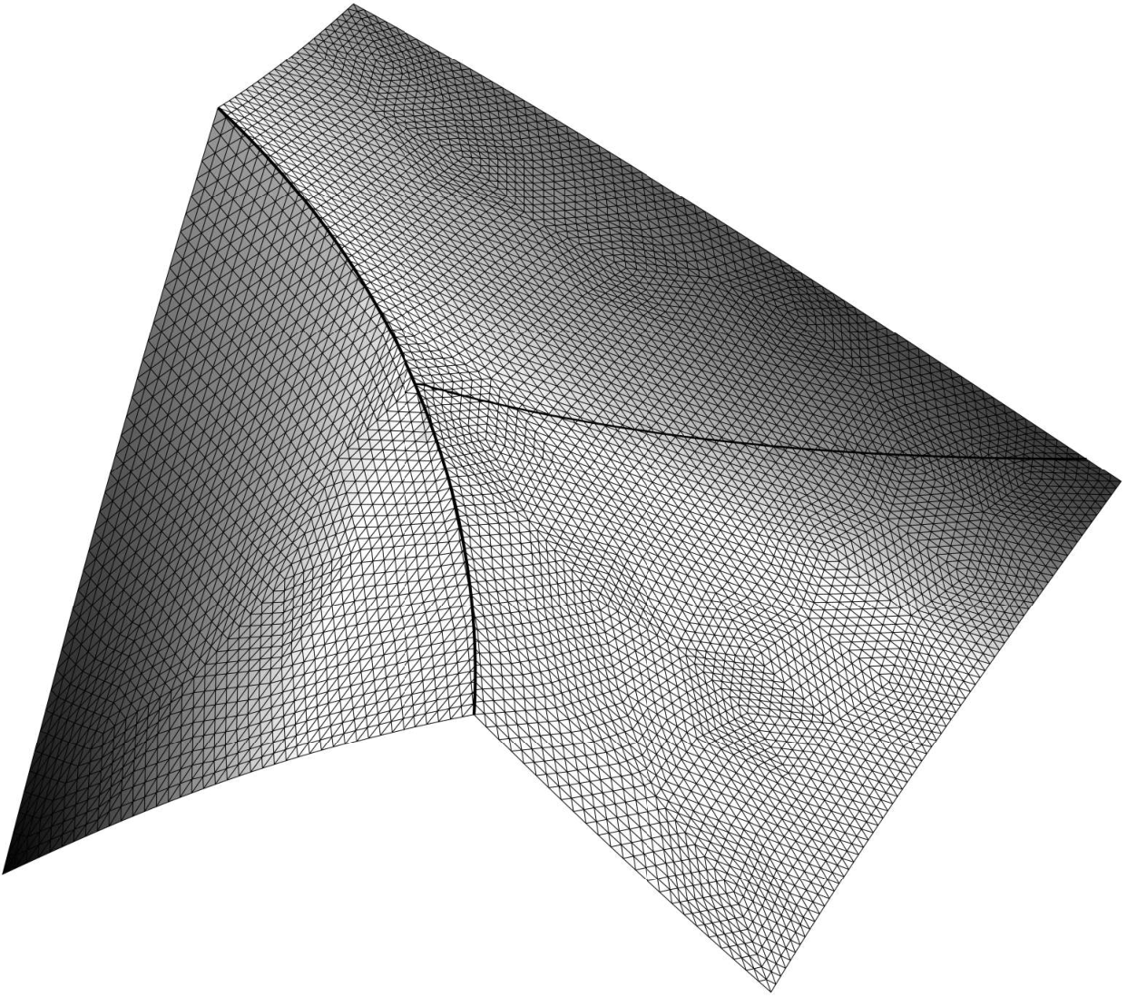
Figure 9: Active meshes with two embedded fractures, Example 2.
Refer to caption
Figure 10: Elevation of the approximate solution with two embedded fractures, Example 2.
Figure 11: L2L_{2}-norm and energy-norm convergence using natural logarithm with two embedded fractures, Example 2. Dotted lines signify optimal convergence. Inclination 1:1 for energy-norm and 2:1 for L2L_{2}-norm.

6.4 Example 3. Flow in Bifurcating Fractures

We consider an example with two bifurcating points. The fractures are modeled using higher order curves. In Figure 12 we show the fractures and construction of individual elements. On the domain Ω\Omega = (0, 1) ×\times (0, 1), we chose a1=a2=1a_{1}=a_{2}=1, fΩ=1f_{\Omega}=1 and fΓ=0f_{\Gamma}=0. We impose the Dirichlet boundary conditions u=0u=0 at x,y=0x,y=0 and u=1u=1 at x,y=1x,y=1. For the diffusion coefficient, we denote aΓia_{\Gamma_{i}} for each fracture and assign an individual value for each Γi\Gamma_{i}, see Figure 13. In Figure 14 through Figure 16, we present the solutions using global refinement with aΓi∈{0,100}a_{\Gamma_{i}}\in\{0,100\}.

Figure 12: Active meshes with two bifurcating points, Example 3.
Figure 13: Embedded fractures with assigned Γ\Gamma, Example 3.
Refer to caption
Figure 14: Elevation of the approximate solution using two bifurcating points, Example 3. Assigned value to the left figure: aΓ1=aΓ2=aΓ3=aΓ4=aΓ5=0a_{\Gamma_{1}}=a_{\Gamma_{2}}=a_{\Gamma_{3}}=a_{\Gamma_{4}}=a_{\Gamma_{5}}=0, and assigned values to the right figure: aΓ1=100a_{\Gamma_{1}}=100 and aΓ2=aΓ3=aΓ4=aΓ5=0a_{\Gamma_{2}}=a_{\Gamma_{3}}=a_{\Gamma_{4}}=a_{\Gamma_{5}}=0.
Refer to caption
Figure 15: Elevation of the approximate solution using two bifurcating points, Example 3. Assigned value to the left figure: aΓ1=aΓ2=100a_{\Gamma_{1}}=a_{\Gamma_{2}}=100 and aΓ3=aΓ4=aΓ5=0a_{\Gamma_{3}}=a_{\Gamma_{4}}=a_{\Gamma_{5}}=0, and assigned values to the right figure: aΓ1=aΓ2=aΓ3=100a_{\Gamma_{1}}=a_{\Gamma_{2}}=a_{\Gamma_{3}}=100 and aΓ4=aΓ5=0a_{\Gamma_{4}}=a_{\Gamma_{5}}=0.
Refer to caption
Figure 16: Elevation of the approximate solution using two bifurcating points, Example 3. Assigned value to the left figure: aΓ1=aΓ2=aΓ3=aΓ4=100a_{\Gamma_{1}}=a_{\Gamma_{2}}=a_{\Gamma_{3}}=a_{\Gamma_{4}}=100 and aΓ5=0a_{\Gamma_{5}}=0, and assigned values to the right figure: aΓ1=aΓ2=aΓ3=aΓ4=aΓ5=100a_{\Gamma_{1}}=a_{\Gamma_{2}}=a_{\Gamma_{3}}=a_{\Gamma_{4}}=a_{\Gamma_{5}}=100.

References

  • [1] P. Angot, F. Boyer, and F. Hubert. Asymptotic and numerical modelling of flows in fractured porous media. ESAIM: Math. Model. Numer. Anal., 43(2):239–275, 2009.
  • [2] E. Burman, S. Claus, P. Hansbo, M. G. Larson, and A. Massing. CutFEM: discretizing geometry and partial differential equations. Internat. J. Numer. Methods Engrg., 104(7):472–501, 2015.
  • [3] E. Burman and P. Hansbo. Fictitious domain finite element methods using cut elements: II. A stabilized Nitsche method. Appl. Numer. Math., 62(4):328–341, 2012.
  • [4] E. Burman, P. Hansbo, and M. G. Larson. A simple finite element method for elliptic bulk problems with embedded surfaces. ArXiv e-prints, Sept. 2017.
  • [5] E. Burman, P. Hansbo, M. G. Larson, and S. Zahedi. Cut finite element methods for coupled bulk-surface problems. Numer. Math., 133(2):203–231, 2016.
  • [6] D. Capatina, R. Luce, H. El-Otmany, and N. Barrau. Nitsche’s extended finite element method for a fracture model in porous media. Appl. Anal., 95(10):2224–2242, 2016.
  • [7] C. D’Angelo and A. Scotti. A mixed finite element method for Darcy flow in fractured porous media with non-matching grids. ESAIM: Math. Model. Numer. Anal., 46(2):465–489, 2012.
  • [8] M. Del Pra, A. Fumagalli, and A. Scotti. Well posedness of fully coupled fracture/bulk Darcy flow with XFEM. SIAM J. Numer. Anal., 55(2):785–811, 2017.
  • [9] L. Formaggia, A. Fumagalli, A. Scotti, and P. Ruffo. A reduced model for Darcy’s problem in networks of fractures. ESAIM: Math. Model. Numer. Anal., 48(4):1089–1116, 2014.
  • [10] N. Frih, J. E. Roberts, and A. Saada. Modeling fractures as interfaces: a model for Forchheimer fractures. Comput. Geosci., 12(1):91–104, 2008.
  • [11] H. Hægland, A. Assteerawatt, H. K. Dahle, G. T. Eigestad, and R. Helmig. Comparison of cell- and vertex-centered discretization methods for flow in a two-dimensional discrete-fracture-matrix system. Adv. Water Resour., 32(12):1740–1755, 2009.
  • [12] A. Hansbo and P. Hansbo. An unfitted finite element method, based on Nitsche’s method, for elliptic interface problems. Comput. Methods Appl. Mech. Engrg., 191(47-48):5537–5552, 2002.
  • [13] P. Hansbo, T. Jonsson, M. G. Larson, and K. Larsson. A Nitsche method for elliptic problems on composite surfaces. Comput. Methods Appl. Mech. Engrg., 326:505–525, 2017.
  • [14] V. Martin, J. Jaffré, and J. E. Roberts. Modeling fractures and barriers as interfaces for flow in porous media. SIAM J. Sci. Comput., 26(5):1667–1691, 2005.

Acknowledgements.

This research was supported in part by the Swedish Foundation for Strategic Research Grant No. AM13-0029, the Swedish Research Council Grants Nos. 2013-4708, 2017-03911, and the Swedish Research Programme Essence. EB was supported in part by the EPSRC grant EP/P01576X/1.

Authors’ addresses:

Erik Burman,   Mathematics, University College London, UK
e.burman@ucl.ac.uk

Peter Hansbo,   Mechanical Engineering, Jönköping University, Sweden
peter.hansbo@ju.se

Mats G. Larson,   Mathematics and Mathematical Statistics, Umeå University, Sweden
mats.larson@umu.se

David Samvin,   Mechanical Engineering, Jönköping University, Sweden
david.samvin@ju.se