跳到论文正文
W Papers独立论文阅读器 arXiv:1805.00429 论文正文 计算阅读时间 · 0%
引用这篇论文根据当前论文元数据生成,正式投稿前建议核对。


License: arXiv.org perpetual non-exclusive license
arXiv:1805.00429v3 [math.GT] 22 May 2019

Trisections of surface complements and the Price twist

Seungwon Kim and Maggie Miller Address: Seungwon Kim
National Institute for Mathematical Sciences
Daejeon, South Korea
Email address: math751@gmail.com Address: Maggie Miller
Department of Mathematics
Princeton University
Princeton, NJ 08544, USA
Email address: maggiem@math.princeton.edu URL: http://www.math.princeton.edu/˜maggiem
Abstract.

Given a real projective plane SS embedded in a 44-manifold X4X^{4} with Euler number 22 or −2-2, the Price twist is a surgery operation on ν⁡(S)\nu(S) yielding (up to) three different 44-manifolds: X4,τS​(X4),ΣS​(X4)X^{4},\tau_{S}(X^{4}),\Sigma_{S}(X^{4}). This is of particular interest when X4=S4X^{4}=S^{4}, as then ΣS​(X4)\Sigma_{S}(X^{4}) is a homotopy 4-sphere which is not obviously diffeomorphic to S4S^{4}. In this paper, we show how to produce a trisection description of each Price twist on S⊂X4S\subset X^{4} by producing a relative trisection of X4∖ν⁡(S)X^{4}\setminus\nu(S). Moreover, we show how to produce a trisection description of general surface complements in 44-manifolds.

1. Introduction

In 2012, Gay and Kirby [GK] introduced trisections of closed 44-manifolds, an analogue of Heegaard splittings of 33-manifolds. During the past six years, topologists have extended this idea to various objects such as 44-manifolds with boundary [C], knotted surfaces in 44-manifolds [MZ2], and finitely presented groups [AGK]. Furthermore, trisections have been used to study classical problems in topology, such as the generalized property R conjecture [MSZ] and the Thom conjecture [L]. Recently, Gay and Meier [GM] have studied surgery on spheres in S4S^{4} (including the Gluck twist and blowdown), by constructing trisections of sphere complements in 44-manifolds. In this paper, we study the Price twist, which is a generalization of the Gluck twist [P] (surgering an ℝ​P2\mathbb{R}P^{2} rather than an S2S^{2}) by constructing trisections of general surface complements in 44-manifolds.

This paper is organized as follows. In Section 2, we give definitions of various notions of trisection. In Section 3, we describe the Price twist. In Section 4, we show how to produce a relative trisection of a surface complement in a 44-manifold. Lastly, in Section 5 we give a procedure that produces a trisection of a 44-manifold arising from a Price twist.

Acknowledgements

Thanks to Jeff Meier, David Gay, and Alex Zupan for helpful conversations about surface complements (especially at CIRM 2018 and BIRS-CMO 2017). Thanks to Selman Akbulut for making us aware of plugs in 44-manifolds at the AMS 2018 Spring Eastern Sectional Meeting. The second author also thanks her graduate advisor, David Gabai. Finally, we thank an anonymous referee for thoroughly reading this paper and providing many helpful comments.

The first author is supported by the National Institute for Mathematical Sciences South Korea (NIMS). The second author is a fellow in the National Science Foundation Graduate Research Fellowship program, under Grant No. DGE-1656466.

2. Trisection, relative trisection, and bridge trisection

2.1. Definitions

First, we define a trisection of a closed 44-manifold.

Definition 2.1.

[GK] Let X4X^{4} be a closed 44-manifold. A (g,k)(g,k)-trisection of X4X^{4} is a triple (X1,X2,X3)(X_{1},X_{2},X_{3}) where

  • •

    X1∪X2∪X3=X4X_{1}\cup X_{2}\cup X_{3}=X^{4},

  • •

    Xi≅♮k​S1×B3X_{i}\cong\natural_{k}S^{1}\times B^{3},

  • •

    Xi∩Xj=∂Xi∩∂Xj≅♮g​S1×B2X_{i}\cap X_{j}=\partial X_{i}\cap\partial X_{j}\cong\natural_{g}S^{1}\times B^{2}

  • •

    X1∩X2∩X3≅ΣgX_{1}\cap X_{2}\cap X_{3}\cong\Sigma_{g},

where Σg\Sigma_{g} is the closed orientable surface of genus gg.

Note that from the definition, (Σg,Xi∩Xj,Xi∩Xk)(\Sigma_{g},X_{i}\cap X_{j},X_{i}\cap X_{k}) gives a Heegaard splitting of ∂Xi≅#k​(S1×S2)\partial X_{i}\cong\#_{k}(S^{1}\times S^{2}). By Laudenbach-Poenaru [LP], X4X^{4} is specified by its spine, (Σg×D2)∪i,j(Xi∩Xj)(\Sigma_{g}\times D^{2})\cup_{i,j}(X_{i}\cap X_{j}). Therefore, we usually describe a trisection (X1,X2,X3)(X_{1},X_{2},X_{3}) by a trisection diagram (Σg,α,β,γ)(\Sigma_{g},\alpha,\beta,\gamma) where each of α,β,\alpha,\beta, and γ\gamma consist of gg independent curves bounding disks in the handlebodies X1∩X2,X2∩X3,X1∩X3X_{1}\cap X_{2},X_{2}\cap X_{3},X_{1}\cap X_{3} respectively. We generally depict this diagram by drawing on Σg\Sigma_{g} the α\alpha curves in red, the β\beta curves in blue, and the γ\gamma curves in green. One typically uses the names Hα:=X1∩X2,Hβ:=X2∩X3,Hγ:=X3∩X1H_{\alpha}:=X_{1}\cap X_{2},H_{\beta}:=X_{2}\cap X_{3},H_{\gamma}:=X_{3}\cap X_{1} for the double intersections. In words, HαH_{\alpha} is usually called “the α\alpha handlebody” (and similarly HβH_{\beta} is the β\beta handlebody and HγH_{\gamma} is the γ\gamma handlebody).

For expositions of trisections, refer to [GK] or [MSZ].

Next, we define a relative trisection of a compact 44-manifold with boundary.

Definition 2.2.

[GK] Let X4X^{4} be a compact 44-manifold with boundary M3≠∅M^{3}\neq\emptyset. A (g,k,p,b)(g,k,p,b)-relative trisection of X4X^{4} is a triple (X1,X2,X3)(X_{1},X_{2},X_{3}) where

  • •

    X1∪X2∪X3=X4X_{1}\cup X_{2}\cup X_{3}=X^{4},

  • •

    Xi≅♮k​S1×B3X_{i}\cong\natural_{k}S^{1}\times B^{3},

  • •

    Xi∩Xj=∂Xi∩∂Xj≅(Σgb×I)∪((g−p)CLOSEX_{i}\cap X_{j}=\partial X_{i}\cap\partial X_{j}\cong(\Sigma_{g}^{b}\times I)\cup((g-p) 22-handles)
    ≅♮g+b+p−1​S1×B2\cong\natural_{g+b+p-1}S^{1}\times B^{2}

  • •

    X1∩X2∩X3≅ΣgbX_{1}\cap X_{2}\cap X_{3}\cong\Sigma_{g}^{b},

where Σgb\Sigma_{g}^{b} is an orientable surface of genus gg and b>0b>0 boundary components. In Xi∩XjX_{i}\cap X_{j}, the (g−p)(g-p) 22-handles are attached to cancel (g−p)(g-p) 11-handles of Σgb×I\Sigma_{g}^{b}\times I. This ensures Xi∩XjX_{i}\cap X_{j} is a 33-dimensional handlebody of genus (g+p+b−1)(g+p+b-1). Moreover, we have the following conditions on M3M^{3}:

  • •

    Xi∩Xj∩M3≅ΣpbX_{i}\cap X_{j}\cap M^{3}\cong\Sigma_{p}^{b},

  • •

    Xi∩M3=(Xi∩Xj∩M3)×IX_{i}\cap M^{3}=(X_{i}\cap X_{j}\cap M^{3})\times I.

Thus, (X1,X2,X3)(X_{1},X_{2},X_{3}) determines an open book decomposition on M3M^{3}, where each Xi∩Xj∩M3X_{i}\cap X_{j}\cap M^{3} is a single page. (In particular, if MM is connected, then Xi∩Xj∩M3X_{i}\cap X_{j}\cap M^{3} must be connected.)

Relative trisections of X4X^{4} and Y4Y^{4} with ∂X4≅∂Y4\partial X^{4}\cong\partial Y^{4} can be glued to form a trisection of X4∪∂Y4X^{4}\cup_{\partial}Y^{4} if and only if the relative trisections induce the same (isotopic) open books on ∂X4≅∂Y4\partial X^{4}\cong\partial Y^{4}, but with opposite orientations [C].

Again, X4X^{4} is specified by its spine, (Σgb×D2)∪i,j(Xi∩Xj)(\Sigma_{g}^{b}\times D^{2})\cup_{i,j}(X_{i}\cap X_{j}) [CGP1]. Therefore, we usually describe a relative trisection (X1,X2,X3)(X_{1},X_{2},X_{3}) by a relative trisection diagram (Σgb,α,β,γ)(\Sigma_{g}^{b},\alpha,\beta,\gamma) where each of α,β,γ\alpha,\beta,\gamma consist of (g−p)(g-p) independent curves bounding disks in the compression bodies X1∩X2,X2∩X3,X1∩X3X_{1}\cap X_{2},X_{2}\cap X_{3},X_{1}\cap X_{3} respectively. We generally depict this diagram by drawing on Σgb\Sigma_{g}^{b} the α\alpha curves in red, the β\beta curves in blue, and the γ\gamma curves in green. One typically uses the names Hα:=X1∩X2,Hβ:=X2∩X3,Hγ:=X3∩X1H_{\alpha}:=X_{1}\cap X_{2},H_{\beta}:=X_{2}\cap X_{3},H_{\gamma}:=X_{3}\cap X_{1} for the double intersections. In words, HαH_{\alpha} is usually called “the α\alpha compression body” (and similarly HβH_{\beta} is the β\beta compression body and HγH_{\gamma} is the γ\gamma compression body).

For expositions of relative trisections, refer to [C], [CGP1] or [CO].

Lastly, we end this section by defining a bridge trisection of a knotted surface in an arbitrary 44-manifold.

Definition 2.3.

Let SS be a surface embedded in a 44-manifold X4X^{4}. Say X4X^{4} has a (g,k)(g,k)-trisection (X1,X2,X3)(X_{1},X_{2},X_{3}). By [MZ2], SS can be isotoped so that

  • •

    S∩XiS\cap X_{i} is a disjoint union of cc-boundary parallel disks,

  • •

    S∩Xi∩XjS\cap X_{i}\cap X_{j} is a trivial tangle of bb arcs.

Note χ⁡(S)=3​c−b\chi(S)=3c-b. We say SS is in(c,b)(c,b)-bridge position in X4X^{4} with respect to (X1,X2,X3)(X_{1},X_{2},X_{3}), or that (X1,X2,X3)(X_{1},X_{2},X_{3}) induces a (c,b)(c,b)-bridge trisection on SS. We can stabilize (X1,X2,X3)(X_{1},X_{2},X_{3}) to find a trisection (X~1,X~2,X~3)(\mathchoice{\accentset{\displaystyle\text{\smash{\raisebox{-5.59721pt}{$\wtilde$}}}}{X}}{\accentset{\textstyle\text{\smash{\raisebox{-5.59721pt}{$\wtilde$}}}}{X}}{\accentset{\scriptstyle\text{\smash{\raisebox{-3.91806pt}{$\wtilde$}}}}{X}}{\accentset{\scriptscriptstyle\text{\smash{\raisebox{-2.7986pt}{$\wtilde$}}}}{X}}_{1},\mathchoice{\accentset{\displaystyle\text{\smash{\raisebox{-5.59721pt}{$\wtilde$}}}}{X}}{\accentset{\textstyle\text{\smash{\raisebox{-5.59721pt}{$\wtilde$}}}}{X}}{\accentset{\scriptstyle\text{\smash{\raisebox{-3.91806pt}{$\wtilde$}}}}{X}}{\accentset{\scriptscriptstyle\text{\smash{\raisebox{-2.7986pt}{$\wtilde$}}}}{X}}_{2},\mathchoice{\accentset{\displaystyle\text{\smash{\raisebox{-5.59721pt}{$\wtilde$}}}}{X}}{\accentset{\textstyle\text{\smash{\raisebox{-5.59721pt}{$\wtilde$}}}}{X}}{\accentset{\scriptstyle\text{\smash{\raisebox{-3.91806pt}{$\wtilde$}}}}{X}}{\accentset{\scriptscriptstyle\text{\smash{\raisebox{-2.7986pt}{$\wtilde$}}}}{X}}_{3}) which induces a (1,b−3​(c−1))(1,b-3(c-1))-bridge trisection on SS [MZ2].

For expositions on bridge trisections of surfaces in 44-manifolds, see [MZ1] or [MZ2].

Bridge trisections admit two kinds of diagrams. One is a diagram (in the standard sense) of the triple of tangles (Xi∩Xi+1,S∩Xi∩Xi+1)∣i=1,2,3(X_{i}\cap X_{i+1},S\cap X_{i}\cap X_{i+1})\mid_{i=1,2,3} (where X4:=X1X_{4}:=X_{1}). When g=0g=0, this diagram consists of 33-tangle diagrams in disks. This is usally called a triplane diagram. Another kind of diagram is the shadow diagram. The shadow diagram is less likely to be familiar to the average reader, so we expand more upon its definition.

Definition 2.4.

Let SS be a surface in (c,b)(c,b)-bridge position in X4X^{4} with respect to the (g,k)(g,k)-trisection (X1,X2,X3)(X_{1},X_{2},X_{3}). Let (Σg,α,β,γ)(\Sigma_{g},\alpha,\beta,\gamma) be a trisection diagram of (X1,X2,X3)(X_{1},X_{2},X_{3}). Identify Σg\Sigma_{g} with X1∩X2∩X3X_{1}\cap X_{2}\cap X_{3}. A shadow diagram for SS is a septuple (Σg,α,β,γ,sα,sβ,sγ)(\Sigma_{g},\alpha,\beta,\gamma,s_{\alpha},s_{\beta},s_{\gamma}) where

  • •

    Each s∗s_{*} is a collection of bb disjoint arcs in Σg\Sigma_{g} with ∂s∗=S∩Σg\partial s_{*}=S\cap\Sigma_{g}.

  • •

    The collection of cc circles (S∩(X1∩X2))∪sα(S\cap(X_{1}\cap X_{2}))\cup s_{\alpha} bounds a set of cc disjoint embedded disks DαD_{\alpha} in X1∩X2X_{1}\cap X_{2}, with D̊α∩(∂(X1∩X2))=∅\mathring{D}_{\alpha}\cap(\partial(X_{1}\cap X_{2}))=\emptyset. That is, sαs_{\alpha} can be obtained by projecting the boundary-parallel tangle S∩(X1∩X2)S\cap(X_{1}\cap X_{2}) onto ∂(X1∩X2)=Σ\partial(X_{1}\cap X_{2})=\Sigma.

  • •

    Similarly, sβs_{\beta} and sγs_{\gamma} can be obtained by projecting the boundary-parallel tangles S∩(X2∩X3)⊂X2∩X3S\cap(X_{2}\cap X_{3})\subset X_{2}\cap X_{3} and S∩(X1∩X3)⊂X1∩X3S\cap(X_{1}\cap X_{3})\subset X_{1}\cap X_{3} onto Σg\Sigma_{g}, respectively.

In this paper, whenever we draw a shadow diagram (Σg,α,β,γ,sα,sβ,sγ)(\Sigma_{g},\alpha,\beta,\gamma,s_{\alpha},s_{\beta},s_{\gamma}), we will draw the curves α,β,γ\alpha,\beta,\gamma and arcs sα,sβ,sγs_{\alpha},s_{\beta},s_{\gamma} on the surface Σ\Sigma. The α\alpha curves and sαs_{\alpha} arcs will be red; the β\beta curves and sβs_{\beta} arcs will be blue; the γ\gamma curves and sγs_{\gamma} arcs will be green. The endpoints of s∗s_{*} will be indicated with black dots. See Figure 1 for a small example of a shadow diagram.
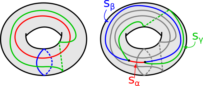
Refer to caption
Figure 1. Left: A trisection diagram (Σ1,α,β,γ)(\Sigma_{1},\alpha,\beta,\gamma) for ℂ​P2\mathbb{C}P^{2}. Right: A shadow diagram (Σ1,α,β,γ,sα,sβ,sγ)(\Sigma_{1},\alpha,\beta,\gamma,s_{\alpha},s_{\beta},s_{\gamma}) for a surface in ℂ​P2\mathbb{C}P^{2}. The α,β,\alpha,\beta, and γ\gamma curves are visible in the left diagram, so we dim them here to make the shadow arcs s∗s_{*} more visible. The described surface is in (1,1)(1,1)-bridge position, so the surface is a sphere. (In fact, this is a shadow diagram for the standard ℂ​P1\mathbb{C}P^{1}.)

The shadow diagram (Σg,α,β,γ,sα,sβ,sγ)(\Sigma_{g},\alpha,\beta,\gamma,s_{\alpha},s_{\beta},s_{\gamma}) determines each Xi∩XjX_{i}\cap X_{j} (up to diffeomorphism) and S∩(Xi∩Xj)S\cap(X_{i}\cap X_{j}) (up to isotopy). Since S∩XiS\cap X_{i} consists of boundary-parallel disks, this determines SS up to isotopy.

See [MZ1] and [MZ2] for the original definitions of triplane and shadow diagrams and many examples.

2.2. Kirby diagrams from relative trisections

In this subsection, we discuss how to obtain a Kirby diagram of X4X^{4} from a relative trisection of X4X^{4}. This essentially comes from Lemma 14 of [GK] (although they only consider closed manifolds, the procedure is almost exactly the same for manifolds with boundary). An alternate viewpoint is found in [MSZ].

Let (Σ,α,β,γ)(\Sigma,\alpha,\beta,\gamma) be a (g,k,p,b)(g,k,p,b)-relative trisection of X4X^{4}. Consider the following handle structure on X4X^{4}:

  • •

    One 00-handle and kk 11-handles, glued to make X1X_{1}.

  • •

    (g−k+p+b−1)(g-k+p+b-1) 22-handles, corresponding to γ\gamma curves which are dual to the β\beta curves (up to handle slides). These handles are glued to the 00- and 11-handles so that X2=(Hβ×I)∪(2CLOSEX_{2}=(H_{\beta}\times I)\cup(2-handles).

  • •

    (k−2​p−b+1)(k-2p-b+1) 33-handles, corresponding to parallel (up to handle slides) α,γ\alpha,\gamma curves. Then X3=((Hα∪ΣHγ)×I)∪(3X_{3}=((H_{\alpha}\cup_{\Sigma}H_{\gamma})\times I)\cup(3-handles).

In pratice, drawing the Kirby diagram for this handle decomposition is simple when there are no 33-handles (i. e. k−2​p−b+1=0k-2p-b+1=0; i. e. there are no parallel α,γ\alpha,\gamma curves). Perform handle-slides on the α,β\alpha,\beta curves so that the pair (α,β)(\alpha,\beta) is standard. Then draw a 11-handle for each cut arc in the α,β\alpha,\beta pages and for each parallel α,β\alpha,\beta curve; draw a 22-handle for each γ\gamma curve with framing given by the surface framing. See Figure 2.

In the above procedure, the 22-handles, 33-handles, and the 11-handles corresponding to parallel α\alpha and β\beta curves should be familiar to a reader who has seen the construction of a Kirby diagram for a closed 44-manifold from a trisection [GK]. The 11-handles corresponding to cut arcs are more novel. These are apparent by actually considering the gluing Hα∪ΣHβH_{\alpha}\cup_{\Sigma}H_{\beta}. Take Hβ=Σ×[0,1]∪(2CLOSEH_{\beta}=\Sigma\times[0,1]\cup(2-handles along OPENβ×0)\beta\times 0) to be the standard compression body in S3S^{3} (see Figure 3). For each α\alpha curve dual to a β\beta curve, a 22-handle can be glued to α×1\alpha\times 1 in S3S^{3}. For each α\alpha curve parallel to a β\beta curve, we add a parallel dotted circle and attach a 22-handle along (α×1)(\alpha\times 1) in #k−2​p−b+1​S1×S2\#_{k-2p-b+1}S^{1}\times S^{2}. This yields Hα∪ΣHβ⊂#k−2​p−b+1S1×S2H_{\alpha}\cup_{\Sigma}H_{\beta}\subset\#_{k-2p-b+1}S^{1}\times S^{2}.

The boundary of Hα∪ΣHβH_{\alpha}\cup_{\Sigma}H_{\beta} consists of the α\alpha and β\beta pages glued together along collars of their boundary, so ∂(Hα∪ΣHβ)\partial(H_{\alpha}\cup_{\Sigma}H_{\beta}) is a surface of genus-(2​p+b−1)(2p+b-1). Moreover, (#k+2​p+b−1S1×S2)∖(Hα∪ΣHβ)(\#_{k+2p+b-1}S^{1}\times S^{2})\setminus(H_{\alpha}\cup_{\Sigma}H_{\beta}) is a handlebody of genus-(2​p+b−1)(2p+b-1). The dotted circles obtained from the cut arcs of the α\alpha and β\beta pages are cores of this handlebody (see Figure 3). Add these dotted circles to the diagram so that now Hα∪ΣHβH_{\alpha}\cup_{\Sigma}H_{\beta} is embedded in #k​S1×S2\#_{k}S^{1}\times S^{2}, so that (#kS1×S2)∖(Hα∪ΣHβ)\#_{k}S^{1}\times S^{2})\setminus(H_{\alpha}\cup_{\Sigma}H_{\beta}) is a product from the α\alpha page to the β\beta page. The total #k​S1×S2\#_{k}S^{1}\times S^{2} is then exactly ∂X1\partial X_{1}.

We take X2X_{2} to be the trace of a cobordism from HβH_{\beta} to HγH_{\gamma}; thicken the β\beta compression body and glue 22-handles for each γ\gamma curve that is dual to the β\beta curves (up to handle slides). By adding 22-handle attaching circles parallel to these γ\gamma curves (with framing equal to the surface framing), we can view X1X_{1} and X2X_{2} as living in the 44-manifold described by this Kirby diagram. Finally, to include X3X_{3} in this diagram we attach 33-handles along essential spheres in Hα∪ΣHγH_{\alpha}\cup_{\Sigma}H_{\gamma} (i.e. one 33-handle for each γ\gamma curve parallel to an α\alpha curve, up to handle slides.)

Refer to caption
Refer to caption
Refer to caption
Figure 2. Top left: a (g,k,p,b)=(3,3,1,2)(g,k,p,b)=(3,3,1,2)-trisection diagram. Here, α\alpha and β\beta are standard. We have drawn a cut-system (purple) for the α\alpha and β\beta pages. Top right: We find a Kirby diagram for the pictured 44-manifold. Each cut arc doubles to a 11-handle curve; push one copy into the α\alpha compression body (“outside the surface”) and the other into the β\beta-compression body (“inside the surface”). The γ\gamma curves become 22-handle attaching circles with framing given by the surface framing. There are no 33- or 44-handles. Bottom: We can now easily see that the pictured 44-manifold is (S2×D2)​♮​(S1×B3)​♮​(S1×B3)(S^{2}\times D^{2})\natural(S^{1}\times B^{3})\natural(S^{1}\times B^{3}).
Refer to caption
Figure 3. We still consider the relative trisection of Figure 2. Left: Hα∪ΣHβH_{\alpha}\cup_{\Sigma}H_{\beta} lies inside #k−2​p−b+1​S1×S2\#_{k-2p-b+1}S^{1}\times S^{2}. The complement of Hα∪ΣHβH_{\alpha}\cup_{\Sigma}H_{\beta} is a handlebody; we have drawn the spine. Right: We isotope the spine to see cores of the handlebody (#k−2​p−b+1S1×S2)∖(Hα∪ΣHβ)(\#_{k-2p-b+1}S^{1}\times S^{2})\setminus(H_{\alpha}\cup_{\Sigma}H_{\beta}) as doubles of a cut system of the α\alpha and β\beta pages.

Finding a relative trisection of X4X^{4} from a Kirby diagram is more challenging. In [CGP2] Castro, Gay, and Pinzón-Caicedo describe how to obtain a relative trisection from a Kirby diagram of X4X^{4} and a page of an open-book on ∂X4\partial X^{4} within the diagram.

3. The Price Twist

3.1. Introduction

Let SS be a real projective plane embedded in a 44-manifold X4X^{4}, with Euler number e⁡(S)=±2e(S)=\pm 2 (e. g. any ℝ​P2\mathbb{R}P^{2} in S4S^{4}). A tubular neighborhood of SS admits a handle structure consisting of a 00-handle, a 11-handle, and a 00-framed 22-handle running twice over the 11-handle (Figure 4). We call this tubular neighborhood P+P_{+} or P−P_{-}, depending on the sign of e⁡(S)e(S). The boundary of PP is the quaternion space QQ, named because it is the quotient of S3S^{3} by the action of the quaternion group. A perhaps more useful description for low-dimensional topologists is that QQ is a Seifert-fibered space over S2S^{2}, with three exceptional fibers of index ±2,±2,∓2\pm 2,\pm 2,\mp 2. Following [KSTY], we call these fibers S0,S1,S−1S_{0},S_{1},S_{-1}. We do not specify the indices of these fibers, as they may be permuted by a homeomorphism of QQ. See Figure 4 for an illustration of S0,S1,S−1S_{0},S_{1},S_{-1} in Q=∂P−Q=\partial P_{-}.

Refer to caption
Figure 4. A kirby diagram of P−P_{-}. (Mirror the diagram to obtain P+P_{+}). Q=∂P±Q=\partial P_{\pm} is a Seifert fibered space with three singular fibers S0,S1,S−1S_{0},S_{1},S_{-1} as pictured. The S−1S_{-1} fiber bounds a disk in P±P_{\pm}.

Note ∂(X4∖ν⁡(S))≅Q\partial(X^{4}\setminus\nu(S))\cong Q. Label the singular fibers in ∂(X4∖ν⁡(S))\partial(X^{4}\setminus\nu(S)) so that the trivial regluing of ν⁡(S)\nu(S) to obtain X4X^{4} corresponds to the map ∂(ν⁡(S))→∂(X4∖S)\partial(\nu(S))\to\partial(X^{4}\setminus S) given by (S1,S0,S−1)↦(S1,S0,S−1)(S_{1},S_{0},S_{-1})\mapsto(S_{1},S_{0},S_{-1})

Price [P] has classified the self-homeomorphisms of QQ, finding that there are six up to isotopy. These maps preserve the Seifert fiber structure, and are determined simply by the induced permutation of the singular fibers. Moreover, Price showed that the map that permutes S0,S1S_{0},S_{1} extends over P±P_{\pm}. Therefore, there are at most three 44-manifolds (up to diffeomorphism) that may arise from deleting ν⁡(S)\nu(S) from X4X^{4} and regluing according to ϕ:∂ν⁡(S)→∂(X4∖ν⁡(S))\phi:\partial\nu(S)\to\partial(X^{4}\setminus\nu(S)). These 44-manifolds are:

  • •

    X4X^{4}, when ϕ⁡(S−1)=S−1\phi(S_{-1})=S_{-1}.

  • •

    τS​(X4)\tau_{S}(X^{4}), when ϕ⁡(S−1)=S0\phi(S_{-1})=S_{0}. Using the Mayer-Vietoris sequence, we see H1​(τS​(X4))≠H1​(X4)H_{1}(\tau_{S}(X^{4}))\neq H_{1}(X^{4}).

  • •

    ΣS​(X4)\Sigma_{S}(X^{4}), when ϕ⁡(S−1)=S1\phi(S_{-1})=S_{1}.

We call ΣS​(X4)\Sigma_{S}(X^{4}) the Price twist of X4X^{4} along SS. In the notation of Akbulut and Yasui [AY], this operation is equivalent to a certain plug twist. See [AY], [A2] for more on this point of view. For our purposes, it is enough to notice that the Price twist is a way of constructing potentially exotic 44-manifolds, and is most interesting in the case X4=S4X^{4}=S^{4}. When X4=S4X^{4}=S^{4}, ΣS​(S4)\Sigma_{S}(S^{4}) is a homotopy 44-sphere. It is unknown under which conditions ΣS​(X4)\Sigma_{S}(X^{4}) is diffeomorphic to X4X^{4}. Katanaga et. al. [KSTY] showed that this operation generalizes the Gluck twist: If KK is a 22-sphere smoothly embedded in X4X^{4} with trivial normal bundle, and PP is a unknotted real projective plane in a 44-ball disjoint from KK, then the Gluck twist of X4X^{4} along KK is diffeomorphic to ΣK​#​P​(X4)\Sigma_{K\#P}(X^{4}). In particular, this means that in some cases ΣS​(X4)≇X4\Sigma_{S}(X^{4})\not\cong X^{4} (see for example [A1]), but there are of course no known examples of this phenomenon in S4S^{4}. (In fact, the authors are unaware of any examples of this phenomenon in any orientable 44-manifold. The surgeries displayed in [A1] which change the smooth structure of the ambient 44-manifold all take place in non-orientable 44-manifolds.) Whether the Price twist strictly generalizes the Gluck twist in S4S^{4} is related to the Kinoshita conjecture.

Question 3.1 (Kinoshita).

Given a real projective plane SS smoothly embedded in S4S^{4}, can SS be decomposed as K​#​PK\#P for some 22-sphere KK and an unknotted real projective plane PP?

The answer to the above question is known to be “yes” in some cases; see e. g. [K1]. One might study the Kinoshita conjecture by understanding the basic algebraic topology of S4∖ν⁡(S)S^{4}\setminus\nu(S). Suppose S=K​#​PS=K\#P for a 22-knot KK and unknotted real projective plane PP. Then S4∖ν⁡(S)≅(S4∖ν⁡(K))​♮​(S4∖ν⁡(P))S^{4}\setminus\nu(S)\cong(S^{4}\setminus\nu(K))\natural(S^{4}\setminus\nu(P)), so π1​(S4∖ν⁡(S))≅π1​(S4∖K∣[γ]2=0)\pi_{1}(S^{4}\setminus\nu(S))\cong\pi_{1}(S^{4}\setminus K\mid[\gamma]^{2}=0), where [γ][\gamma] is a normal generator of π1​(S4∖K)\pi_{1}(S^{4}\setminus K). Fundamental groups of 22-knot complements have been classified as admitting certain presentations by Kamada [K2], so π1​(S4∖ν⁡(S))≅π1​(τS​(S4))\pi_{1}(S^{4}\setminus\nu(S))\cong\pi_{1}(\tau_{S}(S^{4})) is a potential obstruction to SS admitting the decomposition K​#​PK\#P.

3.2. Two preferred trisections of P±P_{\pm}

In this section, we describe two particular (g,k,p,b)=(2,2,0,3)(g,k,p,b)=(2,2,0,3)-relative trisections of P+P_{+} (the mirror images of which are naturally trisections of P−P_{-}), shown in Figure 5. Call these trisections T1T_{1} and T2T_{2}. From TiT_{i}, the dicussion in Section 2.2 yields a Kirby diagram, from which we can check that the trisected manifold is indeed P+P_{+} (see Figure 6). The three singular fibers of Q=∂P+Q=\partial P_{+} form the bindings of the open book induced by TiT_{i} on Q=∂P+Q=\partial P_{+}, and each page has monodromy consisting of two right-handed Dehn twists around two boundary components and two left-handed Dehn twists around the third. In T1T_{1}, the twists around the S−1S_{-1} boundary are left-handed. In T2T_{2}, the twists around the S−1S_{-1} boundary are right-handed (See Figs. 7,8).

Refer to caption
Refer to caption
Figure 5. Left: The relative trisection T1T_{1} of P+P_{+}. Right: the relative trisection T2T_{2} of P+P_{+}. These are both (g,k,p,b)=(2,2,0,3)(g,k,p,b)=(2,2,0,3)-relative trisections.
Refer to caption
Refer to caption
Figure 6. Left: Kirby diagram obtained from T1T_{1}. Right: Kirby diagram obtained from T2T_{2}. Neither diagram has any 33- or 44-handles. Both depict P+P_{+}. The SiS_{i} are the bindings of the open book on QQ (shown here after some handle slides).
Refer to caption
Refer to caption
Figure 7. We perform the algorithm of [CGP1] to find the monodromy of the open book induced on QQ by T1T_{1}. Left: resulting cut systems for each page Xi∩Xj∩∂P+X_{i}\cap X_{j}\cap\partial P_{+}. Right: the effect of the monodromy on the X1∩X2∩∂P+X_{1}\cap X_{2}\cap\partial P_{+} system. The monodromy automorphism consists of two right-handed Dehn twists around each of S0,S1S_{0},S_{1} and two left-handed twists around S−1S_{-1}.
Refer to caption
Refer to caption
Figure 8. We perform the algorithm of [CGP1] to find the monodromy of the open book induced on QQ by T2T_{2}. Left: resulting cut systems for each page Xi∩Xj∩∂P−X_{i}\cap X_{j}\cap\partial P_{-}. Right: the effect of the monodromy on the X1∩X2∩∂P+X_{1}\cap X_{2}\cap\partial P_{+} system. The monodromy automorphism consists of two right-handed Dehn twists around each of S0,S−1S_{0},S_{-1} and two left-handed twists around S1S_{1}.

4. Relative trisections of surface complements

In this section, we show how to produce a relative trisection of the complement of a surface SS in a 44-manifold X4X^{4}. In particular, we can produce a (g,k,p,b)=(g,k,0,3)(g,k,p,b)=(g,k,0,3)-trisection of any ℝ​P2\mathbb{R}P^{2} complement in X4X^{4}. For notational ease, we will often use the shorthand “∩⁣∂\cap\partial” to denote “∩∂(X4∖ν(S))\cap\partial(X^{4}\setminus\nu(S))”.

Naively, one might attempt to construct a trisection of a surface complement in the following (generally incorrect) way.

  • •

    Say X4X^{4} is a 44-manifold with trisection (X1,X2,X3)(X_{1},X_{2},X_{3}).

  • •

    Let S⊂X4S\subset X^{4} be a surface in (c,b)(c,b)-bridge position with respect to the trisection (X1,X2,X3)(X_{1},X_{2},X_{3}).

  • •

    Delete a tubular neighborhood of SS from each XiX_{i} to find a trisection on X4∖ν⁡(S)X^{4}\setminus\nu(S).

This procedure is successful exactly when S≅S2S\cong S^{2} and c=1c=1 (as in [GM]). Otherwise, this procedure does not yield a relative trisection of X4∖ν⁡(S)X^{4}\setminus\nu(S) for (in part) the following reason. Recall from Definition 2.2 that a relative trisection must induce an open book on the 33-dimensional boundary, with pages Xi∩Xj∩∂X_{i}\cap X_{j}\cap\partial. In this setting, ((Xi∩Xj)∖ν(S))∩∂(X4∖ν(S))≅⊔b(S1×I)((X_{i}\cap X_{j})\setminus\nu(S))\cap\partial(X^{4}\setminus\nu(S))\cong\sqcup_{b}(S^{1}\times I), which is a collection of bb annuli corresponding to the bridges of SS in Xi∩XjX_{i}\cap X_{j}. Note that if b=1b=1, then SS is a sphere, since χ⁡(S)=3​c−b\chi(S)=3c-b. If b>1b>1, then ((Xi∩Xj)∖ν⁡(S))∩∂(X4∖ν⁡(S))((X_{i}\cap X_{j})\setminus\nu(S))\cap\partial(X^{4}\setminus\nu(S)) is disconnected, and certainly cannot be a page in an open book on ∂(X4∖(S))\partial(X^{4}\setminus(S)).

To deal with this problem, we introduce an operation on manifolds Y4Y^{4} divided into three pieces Y4=Y1∪Y2∪Y3Y^{4}=Y_{1}\cup Y_{2}\cup Y_{3} (not necessarily as a relative trisection, but still assuming Yi∩Yj=∂Yi∩∂YjY_{i}\cap Y_{j}=\partial Y_{i}\cap\partial Y_{j}) that can reduce the number of components of Yi∩Yj∩∂Y4Y_{i}\cap Y_{j}\cap\partial Y^{4}.

Definition 4.1.

Let Y4Y^{4} be a 44-manifold with nonempty boundary. Let Y4=Y1∪Y2∪Y3Y^{4}=Y_{1}\cup Y_{2}\cup Y_{3}, where Yi∩Yj=∂Yi∩∂YjY_{i}\cap Y_{j}=\partial Y_{i}\cap\partial Y_{j}. Let CC be an arc properly embedded in Yi∩Yj∩∂Y4Y_{i}\cap Y_{j}\cap\partial Y^{4} with endpoints in Y1∩Y2∩Y3Y_{1}\cap Y_{2}\cap Y_{3}. Let ν⁡(C)\nu(C) be a fixed open tubular neighborhood of CC. Let

  • •

    Y~i:=Yi∖ν⁡(C)\mathchoice{\accentset{\displaystyle\text{\smash{\raisebox{-5.59721pt}{$\wtilde$}}}}{Y}}{\accentset{\textstyle\text{\smash{\raisebox{-5.59721pt}{$\wtilde$}}}}{Y}}{\accentset{\scriptstyle\text{\smash{\raisebox{-3.91806pt}{$\wtilde$}}}}{Y}}{\accentset{\scriptscriptstyle\text{\smash{\raisebox{-2.7986pt}{$\wtilde$}}}}{Y}}_{i}:=Y_{i}\setminus\nu(C),

  • •

    Y~j:=Yj∖ν⁡(C)\mathchoice{\accentset{\displaystyle\text{\smash{\raisebox{-5.59721pt}{$\wtilde$}}}}{Y}}{\accentset{\textstyle\text{\smash{\raisebox{-5.59721pt}{$\wtilde$}}}}{Y}}{\accentset{\scriptstyle\text{\smash{\raisebox{-3.91806pt}{$\wtilde$}}}}{Y}}{\accentset{\scriptscriptstyle\text{\smash{\raisebox{-2.7986pt}{$\wtilde$}}}}{Y}}_{j}:=Y_{j}\setminus\nu(C),

  • •

    Y~k:=Yk∪ν⁡(C)¯\mathchoice{\accentset{\displaystyle\text{\smash{\raisebox{-5.59721pt}{$\wtilde$}}}}{Y}}{\accentset{\textstyle\text{\smash{\raisebox{-5.59721pt}{$\wtilde$}}}}{Y}}{\accentset{\scriptstyle\text{\smash{\raisebox{-3.91806pt}{$\wtilde$}}}}{Y}}{\accentset{\scriptscriptstyle\text{\smash{\raisebox{-2.7986pt}{$\wtilde$}}}}{Y}}_{k}:=Y_{k}\cup\overline{\nu(C)}.

We refer to the replacement of the triple (Y1,Y2,Y3)(Y_{1},Y_{2},Y_{3}) by (Y~1,Y~2,Y~3)(\mathchoice{\accentset{\displaystyle\text{\smash{\raisebox{-5.59721pt}{$\wtilde$}}}}{Y}}{\accentset{\textstyle\text{\smash{\raisebox{-5.59721pt}{$\wtilde$}}}}{Y}}{\accentset{\scriptstyle\text{\smash{\raisebox{-3.91806pt}{$\wtilde$}}}}{Y}}{\accentset{\scriptscriptstyle\text{\smash{\raisebox{-2.7986pt}{$\wtilde$}}}}{Y}}_{1},\mathchoice{\accentset{\displaystyle\text{\smash{\raisebox{-5.59721pt}{$\wtilde$}}}}{Y}}{\accentset{\textstyle\text{\smash{\raisebox{-5.59721pt}{$\wtilde$}}}}{Y}}{\accentset{\scriptstyle\text{\smash{\raisebox{-3.91806pt}{$\wtilde$}}}}{Y}}{\accentset{\scriptscriptstyle\text{\smash{\raisebox{-2.7986pt}{$\wtilde$}}}}{Y}}_{2},\mathchoice{\accentset{\displaystyle\text{\smash{\raisebox{-5.59721pt}{$\wtilde$}}}}{Y}}{\accentset{\textstyle\text{\smash{\raisebox{-5.59721pt}{$\wtilde$}}}}{Y}}{\accentset{\scriptstyle\text{\smash{\raisebox{-3.91806pt}{$\wtilde$}}}}{Y}}{\accentset{\scriptscriptstyle\text{\smash{\raisebox{-2.7986pt}{$\wtilde$}}}}{Y}}_{3}) as a boundary-stabilization. We say that we have boundary-stabilized YkY_{k}.

This move is depicted in Figure 11.

We illustrate the effect of this stabilization on each of Y1,Y2,Y3Y_{1},Y_{2},Y_{3}, double intersection, and triple intersection by studying trisections of ℝ​P2\mathbb{R}P^{2} complements in the following subsection. In Section 4.2, we will use the same principle to trisect the complement of an arbitrary surface complement.

4.1. Trisecting complements of embedded ℝ​P2\mathbb{R}P^{2}s

Let (X1,X2,X3)(X_{1},X_{2},X_{3}) be a (g,k)(g,k)-trisection of X4X^{4}. Let SS be an embedded ℝ​P2\mathbb{R}P^{2} in XX. By [MZ2], SS can be isotoped to be in bridge position with respect to (X1,X2,X3)(X_{1},X_{2},X_{3}). We stabilize the trisection as in [MZ2] so that S∩Xi=D2S\cap X_{i}=D^{2} for each ii. Then S∩Xi∩XjS\cap X_{i}\cap X_{j} is a trivial 22-bridge tangle.

Delete a tubular neighborhood of SS from X4X^{4}; let Xi′:=Xi∖ν⁡(S)X^{\prime}_{i}:=X_{i}\setminus\nu(S). For each i=1,2,3i=1,2,3, with {i,j,k}={1,2,3}\{i,j,k\}=\{1,2,3\}, let CiC_{i} be an arc in Xj′∩Xk′∩∂(X4∖ν⁡(S))X^{\prime}_{j}\cap X^{\prime}_{k}\cap\partial(X^{4}\setminus\nu(S)) (with endpoints in OPENX1′∩X2′∩X3′)X^{\prime}_{1}\cap X^{\prime}_{2}\cap X^{\prime}_{3}) which meets two different boundary components of X1′∩X2′∩X3′X^{\prime}_{1}\cap X^{\prime}_{2}\cap X^{\prime}_{3}. Take C1,C2,C3C_{1},C_{2},C_{3} to have disjoint endpoints, and to twist zero times around the 33-dimensional tubes of ν⁡(S)∩(Xi∩Xj)\nu(S)\cap(X_{i}\cap X_{j}) (i.e. we ask S∩(Xi∩Xj)S\cap(X_{i}\cap X_{j}) cobounds disks DD in Xi∩XjX_{i}\cap X_{j} with arcs in Xi∩Xj∩XkX_{i}\cap X_{j}\cap X_{k} so that Ck∩D=∅C_{k}\cap D=\emptyset). This will not matter until we attempt to find the resulting relative trisection diagram. In principal, one could allow CiC_{i} to twist around ν⁡(S)∩(Xj∩Xk)\nu(S)\cap(X_{j}\cap X_{k}) arbitrarily and modify the relative trisection accordingly, but for simplicitly we restrict the intersection). We will boundary-stabilize each XiX_{i} along CiC_{i} to find a relative trisection of X4∖ν⁡(S)X^{4}\setminus\nu(S).

The boundary-stabilization move of X3′X^{\prime}_{3} along C:=C3C:=C_{3} is pictured in Figures 10 and 11. For ease of discussion, we write ν⁡(C)¯=[−ϵ,1+ϵ]×B\overline{\nu(C)}=[-\epsilon,1+\epsilon]\times B, where BB is a (closed) half 33-ball. Write ∂B=D+∪D−\partial B=D_{+}\cup D_{-}, where D+D_{+} and D−D_{-} are each disks, and ν⁡(C)∩∂(X4∖ν⁡(S))=[−ϵ,1+ϵ]×D−\nu(C)\cap\partial(X^{4}\setminus\nu(S))=[-\epsilon,1+\epsilon]\times D_{-}. Write BB as the union of two quarter (closed) 33-balls B1B_{1} and B2B_{2} along a disk so that ν⁡(C)¯∩X1′=I×B1\overline{\nu(C)}\cap X^{\prime}_{1}=I\times B_{1}, ν⁡(C)¯∩X2′=I×B2\overline{\nu(C)}\cap X^{\prime}_{2}=I\times B_{2}, and ν⁡(C)¯∩X3′=([−ϵ,0]∪[1,1+ϵ])×B\overline{\nu(C)}\cap X^{\prime}_{3}=([-\epsilon,0]\cup[1,1+\epsilon])\times B. See Figure 9.

Refer to caption
Figure 9. To understand the effect of boundary-stabilizing along arc CC in X′1∩X′2∩∂X^{\prime}_{1}\cap X^{\prime}_{2}\cap\partial, we write ν⁡(C)¯\overline{\nu(C)} as [−ϵ,1+ϵ]×B[-\epsilon,1+\epsilon]\times B, where BB is a closed half 33-ball. Here, we draw BB. We decompose BB into two quarter-balls B1B_{1} and B2B_{2}, so that ν⁡(C)¯∩X1′=I×B1\overline{\nu(C)}\cap X^{\prime}_{1}=I\times B_{1} and ν⁡(C)¯∩X2′=I×B2\overline{\nu(C)}\cap X^{\prime}_{2}=I\times B_{2}. The boundary of BB is decomposed into two disks, D−D_{-} and D+D_{+} (which both meet B1B_{1} and B2B_{2}) so that ν⁡(C)¯∩∂=[−ϵ,1+ϵ]×D−\overline{\nu(C)}\cap\partial=[-\epsilon,1+\epsilon]\times D_{-}.

This boundary-stabilization increases the genus of X3′X^{\prime}_{3}, X1′∩X3′X^{\prime}_{1}\cap X^{\prime}_{3} and X2′∩X3′X^{\prime}_{2}\cap X^{\prime}_{3} each by one. We illustrate the effect on the Xi′∩Xj′∩∂(X4∖ν⁡(S))X^{\prime}_{i}\cap X^{\prime}_{j}\cap\partial(X^{4}\setminus\nu(S)) and X1′∩X2′∩X3′X^{\prime}_{1}\cap X^{\prime}_{2}\cap X^{\prime}_{3} in Figures 12 and 13; each of these figures relate to a schematic triplane diagram. We discuss the topology of each trisection piece before and after the boundary-stabilization move in greater detail in the following paragraphs. (Many of these paragraphs are repetitive due to the symmetry of a trisection, but we consider each piece separately for clarity.) Recall the notation “∩⁣∂\cap\partial” means “∩∂(X4∖ν(S))\cap\partial(X^{4}\setminus\nu(S))”.

Refer to caption
Figure 10. Left: S∩X1∩X2S\cap X_{1}\cap X_{2}. Right: We find an arc CC in X′1∩X′2∩∂X^{\prime}_{1}\cap X^{\prime}_{2}\cap\partial which meets two different boundary components of X1′∩X2′∩X3′X^{\prime}_{1}\cap X^{\prime}_{2}\cap X^{\prime}_{3} [i. e. an arc that runs along one bridge.]
Refer to caption
Figure 11. Top: The shaded regions are slices of a neighborhood of CC in X4∖ν⁡(S)X^{4}\setminus\nu(S) before stabilizing. Bottom: To boundary-stabilize, we declare this neighborhood is in X3′X^{\prime}_{3}.
Refer to caption
Figure 12. The boundary-stabilization move deletes a band from X1′∩X2′∩∂(X4∖ν⁡(S))X^{\prime}_{1}\cap X^{\prime}_{2}\cap\partial(X^{4}\setminus\nu(S)), and adds a band to each of X′1∩X′3∩∂X^{\prime}_{1}\cap X^{\prime}_{3}\cap\partial and X′2∩X′3∩∂X^{\prime}_{2}\cap X^{\prime}_{3}\cap\partial. These are not literally three instances of the same band. The band deleted from X′1∩X′2∩∂X^{\prime}_{1}\cap X^{\prime}_{2}\cap\partial is I×(B1∩B2∩D−)I\times(B_{1}\cap B_{2}\cap D_{-}). The band added to X′1∩X′3∩∂X^{\prime}_{1}\cap X^{\prime}_{3}\cap\partial is I×(B1∩D+∩D−)I\times(B_{1}\cap D_{+}\cap D_{-}). The band added to X2′∩X3′X^{\prime}_{2}\cap X^{\prime}_{3} is I×(B2∩D+∩D−)I\times(B_{2}\cap D_{+}\cap D_{-}).
Refer to caption
Figure 13. The boundary-stabilization move adds a band I×(B1∩B2∩B+)I\times(B_{1}\cap B_{2}\cap B_{+}) to the triple intersection X1′∩X2′∩X3′X^{\prime}_{1}\cap X^{\prime}_{2}\cap X^{\prime}_{3}.

𝐗𝟏′.\mathbf{X^{\prime}_{1}.} Before boundary-stabilizing X3′X^{\prime}_{3}, X1′≅♮k+1​S1×B3X^{\prime}_{1}\cong\natural_{k+1}S^{1}\times B^{3}. After boundary-stabilizing X3′X^{\prime}_{3}, X1′≅♮k+1​S1×B3X^{\prime}_{1}\cong\natural_{k+1}S^{1}\times B^{3}. From X1′X^{\prime}_{1}, in the boundary-stabilization we carve out a neighborhood of arc CC in ∂X1′\partial X^{\prime}_{1}. This does not change the topology of X1′X^{\prime}_{1}.

𝐗𝟐′.\mathbf{X^{\prime}_{2}.} Before boundary-stabilizing X3′X^{\prime}_{3}, X2′≅♮k+1​S1×B3X^{\prime}_{2}\cong\natural_{k+1}S^{1}\times B^{3}. After boundary-stabilizing X3′X^{\prime}_{3}, X2′≅♮k+1​S1×B3X^{\prime}_{2}\cong\natural_{k+1}S^{1}\times B^{3}. From X2′X^{\prime}_{2}, in the boundary-stabilization we carve out a neighborhood of arc CC in ∂X2′\partial X^{\prime}_{2}. This does not change the topology of X2′X^{\prime}_{2}.

𝐗𝟑′.\mathbf{X^{\prime}_{3}.} Before boundary-stabilizing X3′X^{\prime}_{3}, X1′≅♮k+1​S1×B3X^{\prime}_{1}\cong\natural_{k+1}S^{1}\times B^{3}. After boundary-stabilizing X3′X^{\prime}_{3}, X3′≅♮k+2​S1×B3X^{\prime}_{3}\cong\natural_{k+2}S^{1}\times B^{3}. To X3′X^{\prime}_{3}, we add a neighborhood of arc CC (recall ∂C∈∂X3′\partial C\in\partial X^{\prime}_{3}, C̊∩X3′=∅\mathring{C}\cap X^{\prime}_{3}=\emptyset). The effect is to add another boundary-sum S1×B3S^{1}\times B^{3} component to X3′X^{\prime}_{3}.

𝐗𝟏′∩𝐗𝟐′.\mathbf{X^{\prime}_{1}\cap X^{\prime}_{2}.} Before boundary-stabilizing X3′X^{\prime}_{3}, X1′∩X2′≅♮g+2​S1×B2X^{\prime}_{1}\cap X^{\prime}_{2}\cong\natural_{g+2}S^{1}\times B^{2}. After boundary-stabilizing X3′X^{\prime}_{3}, X1′∩X2′≅♮g+2​S1×B2X^{\prime}_{1}\cap X^{\prime}_{2}\cong\natural_{g+2}S^{1}\times B^{2}. From X1′∩X2′X^{\prime}_{1}\cap X^{\prime}_{2}, in the boundary-stabilization we carve out a neighborhood of arc CC in ∂X1′∩X2′\partial X^{\prime}_{1}\cap X^{\prime}_{2}. This does not change the topology of X1′∩X2′X^{\prime}_{1}\cap X^{\prime}_{2}.

𝐗𝟐′∩𝐗𝟑′.\mathbf{X^{\prime}_{2}\cap X^{\prime}_{3}.} Before boundary-stabilizing X3′X^{\prime}_{3}, X2′∩X3′≅♮g+2​S1×B2X^{\prime}_{2}\cap X^{\prime}_{3}\cong\natural_{g+2}S^{1}\times B^{2}. After boundary-stabilizing X3′X^{\prime}_{3}, X2′∩X3′≅♮g+3​S1×B2X^{\prime}_{2}\cap X^{\prime}_{3}\cong\natural_{g+3}S^{1}\times B^{2}. Then to X2′∩X3′X^{\prime}_{2}\cap X^{\prime}_{3}, in the boundary-stabilization we add I×B2I\times B_{2}. The effect is to add another boundary-sum S1×B2S^{1}\times B^{2} component to X2′∩X3′X^{\prime}_{2}\cap X^{\prime}_{3}.

𝐗𝟏′∩𝐗𝟑′.\mathbf{X^{\prime}_{1}\cap X^{\prime}_{3}.} Before boundary-stabilizing X3′X^{\prime}_{3}, X1′∩X3′≅♮g+2​S1×B2X^{\prime}_{1}\cap X^{\prime}_{3}\cong\natural_{g+2}S^{1}\times B^{2}. After boundary-stabilizing X3′X^{\prime}_{3}, X1′∩X3′≅♮g+3​S1×B2X^{\prime}_{1}\cap X^{\prime}_{3}\cong\natural_{g+3}S^{1}\times B^{2}. To X1′∩X3′X^{\prime}_{1}\cap X^{\prime}_{3}, in the boundary-stabilization we add I×B1I\times B_{1}. The effect is to add another boundary-sum S1×B2S^{1}\times B^{2} component to X1′∩X3′X^{\prime}_{1}\cap X^{\prime}_{3}.

𝐗𝟏′∩𝐗𝟐′∩𝐗𝟑′.\mathbf{X^{\prime}_{1}\cap X^{\prime}_{2}\cap X^{\prime}_{3}.} Before boundary-stabilizing X3′X^{\prime}_{3}, X1′∩X2′∩X3′≅Σg,4X^{\prime}_{1}\cap X^{\prime}_{2}\cap X^{\prime}_{3}\cong\Sigma_{g,4}, a genus-gg surface with 44 open disks deleted. After boundary-stabilizing X3′X^{\prime}_{3}, X1′∩X2′∩X3′≅Σg,4∪(CLOSEX^{\prime}_{1}\cap X^{\prime}_{2}\cap X^{\prime}_{3}\cong\Sigma_{g,4}\cup(a band) To X1′∩X2′∩X3′X^{\prime}_{1}\cap X^{\prime}_{2}\cap X^{\prime}_{3}, we add the band I×(B1∩B2∩D+)I\times(B_{1}\cap B_{2}\cap D_{+}). In thiscase, we have assumed that the band meets two distinct boundary components of Σg,4\Sigma_{g,4}, so the attachment yields Σg+1,3\Sigma_{g+1,3}. Note now that C1C_{1} or C2C_{2} may meet only one boundary component of Σg+1,3\Sigma_{g+1,3}.

𝐗′𝟏∩∂.\mathbf{X^{\prime}_{1}\cap\partial.} Before boundary-stabilizing X3′X^{\prime}_{3}, we have X′1∩∂≅S1×B2X^{\prime}_{1}\cap\partial\cong S^{1}\times B^{2}. After boundary-stabilizing X3′X^{\prime}_{3}, X′1∩∂≅S1×B2X^{\prime}_{1}\cap\partial\cong S^{1}\times B^{2}. From X′1∩∂X^{\prime}_{1}\cap\partial, in the boundary-stabilization we carve out a neighborhood of arc CC in ∂(X1′∩∂)\partial(X^{\prime}_{1}\cap\partial). This does not change the topology of X′1∩∂X^{\prime}_{1}\cap\partial.

𝐗′𝟐∩∂.\mathbf{X^{\prime}_{2}\cap\partial.} Before boundary-stabilizing X3′X^{\prime}_{3}, we have X′2∩∂≅S1×B2X^{\prime}_{2}\cap\partial\cong S^{1}\times B^{2}. After boundary-stabilizing X3′X^{\prime}_{3}, X′2∩∂≅S1×B2X^{\prime}_{2}\cap\partial\cong S^{1}\times B^{2}. From X′2∩∂X^{\prime}_{2}\cap\partial, in the boundary-stabilization we carve out a neighborhood of arc CC in ∂(X2′∩∂)\partial(X^{\prime}_{2}\cap\partial). This does not change the topology of X′2∩∂X^{\prime}_{2}\cap\partial.

𝐗′𝟑∩∂.\mathbf{X^{\prime}_{3}\cap\partial.} Before boundary-stabilizing X3′X^{\prime}_{3}, we have X′3∩∂≅S1×B2X^{\prime}_{3}\cap\partial\cong S^{1}\times B^{2}. After boundary-stabilizing X3′X^{\prime}_{3}, X′3∩∂≅♮2S1×B2X^{\prime}_{3}\cap\partial\cong\natural_{2}S^{1}\times B^{2}. To X′3∩∂X^{\prime}_{3}\cap\partial, we add ν(C)∩∂=(\nu(C)\cap\partial=(arc parallel to OPENC)×D2C)\times D^{2} (recall C⊂X1′∩X2′∩∂XC\subset X^{\prime}_{1}\cap X^{\prime}_{2}\cap\partial X). The effect is to add another boundary-sum S1×B2S^{1}\times B^{2} component to X′3∩∂X^{\prime}_{3}\cap\partial.

𝐗′𝟏∩𝐗′𝟐∩∂.\mathbf{X^{\prime}_{1}\cap X^{\prime}_{2}\cap\partial.} Before boundary-stabilizing X3′X^{\prime}_{3}, X1′∩X2′∩∂≅⊔2S1×I=(X^{\prime}_{1}\cap X^{\prime}_{2}\cap\partial\cong\sqcup_{2}S^{1}\times I=(two annuli). After boundary-stabilizing X3′X^{\prime}_{3}, X1′∩X2′∩∂≅D2⊔(S1×I)X^{\prime}_{1}\cap X^{\prime}_{2}\cap\partial\cong D^{2}\sqcup(S^{1}\times I).From X′1∩X′2∩∂X^{\prime}_{1}\cap X^{\prime}_{2}\cap\partial, in the boundary-stabilization we carve out a neighborhood of arc CC, which is a cocore of one annulus.

𝐗′𝟐∩𝐗′𝟑∩∂.\mathbf{X^{\prime}_{2}\cap X^{\prime}_{3}\cap\partial.} Before boundary-stabilizing X3′X^{\prime}_{3}, X′2∩X′3∩∂≅⊔2S1×I=X^{\prime}_{2}\cap X^{\prime}_{3}\cap\partial\cong\sqcup_{2}S^{1}\times I=(two annuli). After boundary-stabilizing X3′X^{\prime}_{3}, X2′∩X3′∩∂≅(⊔2S1×I)∪(X^{\prime}_{2}\cap X^{\prime}_{3}\cap\partial\cong(\sqcup_{2}S^{1}\times I)\cup(bandOPEN)≅Σ0,3)\cong\Sigma_{0,3}. To X′2∩X′3∩∂X^{\prime}_{2}\cap X^{\prime}_{3}\cap\partial, we add I×(B2∩D+∩D−)I\times(B_{2}\cap D_{+}\cap D_{-}).

𝐗′𝟏∩𝐗′𝟑∩∂.\mathbf{X^{\prime}_{1}\cap X^{\prime}_{3}\cap\partial.} Before boundary-stabilizing X3′X^{\prime}_{3}, X′1∩X′3∩∂≅⊔2S1×I=X^{\prime}_{1}\cap X^{\prime}_{3}\cap\partial\cong\sqcup_{2}S^{1}\times I=(two annuli). After boundary-stabilizing X3′X^{\prime}_{3}, X1′∩X3′∩∂≅(⊔2S1×I)∪(X^{\prime}_{1}\cap X^{\prime}_{3}\cap\partial\cong(\sqcup_{2}S^{1}\times I)\cup(bandOPEN)≅Σ0,3)\cong\Sigma_{0,3}. To X′1∩X′3∩∂X^{\prime}_{1}\cap X^{\prime}_{3}\cap\partial, we add I×(B1∩D+∩D−)I\times(B_{1}\cap D_{+}\cap D_{-}).

𝐗′𝟏∩𝐗′𝟐∩𝐗′𝟑∩∂.\mathbf{X^{\prime}_{1}\cap X^{\prime}_{2}\cap X^{\prime}_{3}\cap\partial.} Before boundary-stabilizing X3′X^{\prime}_{3}, X′1∩X′2∩X′3∩∂≅⊔4S1X^{\prime}_{1}\cap X^{\prime}_{2}\cap X^{\prime}_{3}\cap\partial\cong\sqcup_{4}S^{1}, the boundary components of X1′∩X2′∩X3′X^{\prime}_{1}\cap X^{\prime}_{2}\cap X^{\prime}_{3}. After boundary-stabilizing X3′X^{\prime}_{3}, X′1∩X′2∩X′3∩∂≅⊔3S1X^{\prime}_{1}\cap X^{\prime}_{2}\cap X^{\prime}_{3}\cap\partial\cong\sqcup_{3}S^{1}. During the boundary-stabilization, we surger X′1∩X′2∩X′3∩∂X^{\prime}_{1}\cap X^{\prime}_{2}\cap X^{\prime}_{3}\cap\partial along the two intervals in ν⁡(C)\nu(C). The band we surger along is I×(B1∩B2∩D−)I\times(B_{1}\cap B_{2}\cap D_{-}); we delete neighborhoods of ∂I×(B1∩B2∩D−)\partial I\times(B_{1}\cap B_{2}\cap D_{-}) and glue in the remaining boundary. We assumed that the endpoints of CC met different boundary components of X1′∩X2′∩X3′X^{\prime}_{1}\cap X^{\prime}_{2}\cap X^{\prime}_{3}, which causes the number of components of X′1∩X′2∩X′3∩∂X^{\prime}_{1}\cap X^{\prime}_{2}\cap X^{\prime}_{3}\cap\partial to decrease after the boundary-stabilization. If we did the same procedure on an arc with both endpoints on one boundary component then after the boundary-stabilization we would have had X′1∩X′2∩X′3∩∂=⊔5S1X^{\prime}_{1}\cap X^{\prime}_{2}\cap X^{\prime}_{3}\cap\partial=\sqcup_{5}S^{1}. This concludes the analysis of the effect of boundary-stabilizing X3′X^{\prime}_{3} along C=C3C=C_{3}.

Now similarly boundary-stabilize X1′X^{\prime}_{1} along C1C_{1} and X2′X^{\prime}_{2} along C2C_{2} to obtain X4∖ν⁡(S)=X~1∪X~2∪X~3X^{4}\setminus\nu(S)=\mathchoice{\accentset{\displaystyle\text{\smash{\raisebox{-5.59721pt}{$\wtilde$}}}}{X}}{\accentset{\textstyle\text{\smash{\raisebox{-5.59721pt}{$\wtilde$}}}}{X}}{\accentset{\scriptstyle\text{\smash{\raisebox{-3.91806pt}{$\wtilde$}}}}{X}}{\accentset{\scriptscriptstyle\text{\smash{\raisebox{-2.7986pt}{$\wtilde$}}}}{X}}_{1}\cup\mathchoice{\accentset{\displaystyle\text{\smash{\raisebox{-5.59721pt}{$\wtilde$}}}}{X}}{\accentset{\textstyle\text{\smash{\raisebox{-5.59721pt}{$\wtilde$}}}}{X}}{\accentset{\scriptstyle\text{\smash{\raisebox{-3.91806pt}{$\wtilde$}}}}{X}}{\accentset{\scriptscriptstyle\text{\smash{\raisebox{-2.7986pt}{$\wtilde$}}}}{X}}_{2}\cup\mathchoice{\accentset{\displaystyle\text{\smash{\raisebox{-5.59721pt}{$\wtilde$}}}}{X}}{\accentset{\textstyle\text{\smash{\raisebox{-5.59721pt}{$\wtilde$}}}}{X}}{\accentset{\scriptstyle\text{\smash{\raisebox{-3.91806pt}{$\wtilde$}}}}{X}}{\accentset{\scriptscriptstyle\text{\smash{\raisebox{-2.7986pt}{$\wtilde$}}}}{X}}_{3} (where X~i\mathchoice{\accentset{\displaystyle\text{\smash{\raisebox{-5.59721pt}{$\wtilde$}}}}{X}}{\accentset{\textstyle\text{\smash{\raisebox{-5.59721pt}{$\wtilde$}}}}{X}}{\accentset{\scriptstyle\text{\smash{\raisebox{-3.91806pt}{$\wtilde$}}}}{X}}{\accentset{\scriptscriptstyle\text{\smash{\raisebox{-2.7986pt}{$\wtilde$}}}}{X}}_{i} is obtained from Xi′X^{\prime}_{i} by performing all three boundary stabilizations). The end result will have X~i∩X~j∩∂(X4∖ν⁡(S))=\mathchoice{\accentset{\displaystyle\text{\smash{\raisebox{-5.59721pt}{$\wtilde$}}}}{X}}{\accentset{\textstyle\text{\smash{\raisebox{-5.59721pt}{$\wtilde$}}}}{X}}{\accentset{\scriptstyle\text{\smash{\raisebox{-3.91806pt}{$\wtilde$}}}}{X}}{\accentset{\scriptscriptstyle\text{\smash{\raisebox{-2.7986pt}{$\wtilde$}}}}{X}}_{i}\cap\mathchoice{\accentset{\displaystyle\text{\smash{\raisebox{-5.59721pt}{$\wtilde$}}}}{X}}{\accentset{\textstyle\text{\smash{\raisebox{-5.59721pt}{$\wtilde$}}}}{X}}{\accentset{\scriptstyle\text{\smash{\raisebox{-3.91806pt}{$\wtilde$}}}}{X}}{\accentset{\scriptscriptstyle\text{\smash{\raisebox{-2.7986pt}{$\wtilde$}}}}{X}}_{j}\cap\partial(X^{4}\setminus\nu(S))=(thrice punctured sphere) or (once punctured torus), depending on our choice of arcs C1,C2C_{1},C_{2}, and C3C_{3} (see Figure 14).

One point of these boundary-stabilizations is to ensure that X~i∩X~j∩∂(X4∖ν⁡(S))\mathchoice{\accentset{\displaystyle\text{\smash{\raisebox{-5.59721pt}{$\wtilde$}}}}{X}}{\accentset{\textstyle\text{\smash{\raisebox{-5.59721pt}{$\wtilde$}}}}{X}}{\accentset{\scriptstyle\text{\smash{\raisebox{-3.91806pt}{$\wtilde$}}}}{X}}{\accentset{\scriptscriptstyle\text{\smash{\raisebox{-2.7986pt}{$\wtilde$}}}}{X}}_{i}\cap\mathchoice{\accentset{\displaystyle\text{\smash{\raisebox{-5.59721pt}{$\wtilde$}}}}{X}}{\accentset{\textstyle\text{\smash{\raisebox{-5.59721pt}{$\wtilde$}}}}{X}}{\accentset{\scriptstyle\text{\smash{\raisebox{-3.91806pt}{$\wtilde$}}}}{X}}{\accentset{\scriptscriptstyle\text{\smash{\raisebox{-2.7986pt}{$\wtilde$}}}}{X}}_{j}\cap\partial(X^{4}\setminus\nu(S)) is connected. We must furthermore check that X~i∩∂(X4∖ν⁡(S))\mathchoice{\accentset{\displaystyle\text{\smash{\raisebox{-5.59721pt}{$\wtilde$}}}}{X}}{\accentset{\textstyle\text{\smash{\raisebox{-5.59721pt}{$\wtilde$}}}}{X}}{\accentset{\scriptstyle\text{\smash{\raisebox{-3.91806pt}{$\wtilde$}}}}{X}}{\accentset{\scriptscriptstyle\text{\smash{\raisebox{-2.7986pt}{$\wtilde$}}}}{X}}_{i}\cap\partial(X^{4}\setminus\nu(S)) is a product (X~i∩X~j∩∂(X4∖ν⁡(S)))×I(\mathchoice{\accentset{\displaystyle\text{\smash{\raisebox{-5.59721pt}{$\wtilde$}}}}{X}}{\accentset{\textstyle\text{\smash{\raisebox{-5.59721pt}{$\wtilde$}}}}{X}}{\accentset{\scriptstyle\text{\smash{\raisebox{-3.91806pt}{$\wtilde$}}}}{X}}{\accentset{\scriptscriptstyle\text{\smash{\raisebox{-2.7986pt}{$\wtilde$}}}}{X}}_{i}\cap\mathchoice{\accentset{\displaystyle\text{\smash{\raisebox{-5.59721pt}{$\wtilde$}}}}{X}}{\accentset{\textstyle\text{\smash{\raisebox{-5.59721pt}{$\wtilde$}}}}{X}}{\accentset{\scriptstyle\text{\smash{\raisebox{-3.91806pt}{$\wtilde$}}}}{X}}{\accentset{\scriptscriptstyle\text{\smash{\raisebox{-2.7986pt}{$\wtilde$}}}}{X}}_{j}\cap\partial(X^{4}\setminus\nu(S)))\times I and also a product (X~i∩X~k∩∂(X4∖ν⁡(S)))×I(\mathchoice{\accentset{\displaystyle\text{\smash{\raisebox{-5.59721pt}{$\wtilde$}}}}{X}}{\accentset{\textstyle\text{\smash{\raisebox{-5.59721pt}{$\wtilde$}}}}{X}}{\accentset{\scriptstyle\text{\smash{\raisebox{-3.91806pt}{$\wtilde$}}}}{X}}{\accentset{\scriptscriptstyle\text{\smash{\raisebox{-2.7986pt}{$\wtilde$}}}}{X}}_{i}\cap\mathchoice{\accentset{\displaystyle\text{\smash{\raisebox{-5.59721pt}{$\wtilde$}}}}{X}}{\accentset{\textstyle\text{\smash{\raisebox{-5.59721pt}{$\wtilde$}}}}{X}}{\accentset{\scriptstyle\text{\smash{\raisebox{-3.91806pt}{$\wtilde$}}}}{X}}{\accentset{\scriptscriptstyle\text{\smash{\raisebox{-2.7986pt}{$\wtilde$}}}}{X}}_{k}\cap\partial(X^{4}\setminus\nu(S)))\times I (and that these two product structures agree), so that there is an induced open book on the boundary of X4∖ν⁡(S)X^{4}\setminus\nu(S).

Claim 4.2.

X~1∩∂(X4∖ν⁡(S))\mathchoice{\accentset{\displaystyle\text{\smash{\raisebox{-5.59721pt}{$\wtilde$}}}}{X}}{\accentset{\textstyle\text{\smash{\raisebox{-5.59721pt}{$\wtilde$}}}}{X}}{\accentset{\scriptstyle\text{\smash{\raisebox{-3.91806pt}{$\wtilde$}}}}{X}}{\accentset{\scriptscriptstyle\text{\smash{\raisebox{-2.7986pt}{$\wtilde$}}}}{X}}_{1}\cap\partial(X^{4}\setminus\nu(S)) is a product over X~1∩X~2∩∂(X4∖ν⁡(S))\mathchoice{\accentset{\displaystyle\text{\smash{\raisebox{-5.59721pt}{$\wtilde$}}}}{X}}{\accentset{\textstyle\text{\smash{\raisebox{-5.59721pt}{$\wtilde$}}}}{X}}{\accentset{\scriptstyle\text{\smash{\raisebox{-3.91806pt}{$\wtilde$}}}}{X}}{\accentset{\scriptscriptstyle\text{\smash{\raisebox{-2.7986pt}{$\wtilde$}}}}{X}}_{1}\cap\mathchoice{\accentset{\displaystyle\text{\smash{\raisebox{-5.59721pt}{$\wtilde$}}}}{X}}{\accentset{\textstyle\text{\smash{\raisebox{-5.59721pt}{$\wtilde$}}}}{X}}{\accentset{\scriptstyle\text{\smash{\raisebox{-3.91806pt}{$\wtilde$}}}}{X}}{\accentset{\scriptscriptstyle\text{\smash{\raisebox{-2.7986pt}{$\wtilde$}}}}{X}}_{2}\cap\partial(X^{4}\setminus\nu(S)) and over X~1∩X~3∩∂(X4∖ν⁡(S))\mathchoice{\accentset{\displaystyle\text{\smash{\raisebox{-5.59721pt}{$\wtilde$}}}}{X}}{\accentset{\textstyle\text{\smash{\raisebox{-5.59721pt}{$\wtilde$}}}}{X}}{\accentset{\scriptstyle\text{\smash{\raisebox{-3.91806pt}{$\wtilde$}}}}{X}}{\accentset{\scriptscriptstyle\text{\smash{\raisebox{-2.7986pt}{$\wtilde$}}}}{X}}_{1}\cap\mathchoice{\accentset{\displaystyle\text{\smash{\raisebox{-5.59721pt}{$\wtilde$}}}}{X}}{\accentset{\textstyle\text{\smash{\raisebox{-5.59721pt}{$\wtilde$}}}}{X}}{\accentset{\scriptstyle\text{\smash{\raisebox{-3.91806pt}{$\wtilde$}}}}{X}}{\accentset{\scriptscriptstyle\text{\smash{\raisebox{-2.7986pt}{$\wtilde$}}}}{X}}_{3}\cap\partial(X^{4}\setminus\nu(S)). Moreover, these product structures agree.

Proof.

See Figure 14 for an illustration of this proof.

Before any boundary-stabilizations, X′1∩∂X^{\prime}_{1}\cap\partial is a solid torus. X′1∩X′2∩∂X^{\prime}_{1}\cap X^{\prime}_{2}\cap\partial and X′1∩X′3∩∂X^{\prime}_{1}\cap X^{\prime}_{3}\cap\partial are each disjoint unions of two annuli. The core of each annulus is a longitude of the solid torus X′1∩∂X^{\prime}_{1}\cap\partial.

From the discussion so far of Section 4.1, recall that after performing the X3′X^{\prime}_{3}-boundary stabilization we have

X′1∩∂\displaystyle X^{\prime}_{1}\cap\partial ≅S1×B2,\displaystyle\cong S^{1}\times B^{2},
X′1∩X′2∩∂\displaystyle X^{\prime}_{1}\cap X^{\prime}_{2}\cap\partial ≅D2⊔(S1×I),\displaystyle\cong D^{2}\sqcup(S^{1}\times I),
X′1∩X′3∩∂\displaystyle X^{\prime}_{1}\cap X^{\prime}_{3}\cap\partial ≅⊔2(S1×I)∪(band between the two components)≅Σ0,3.\displaystyle\cong\sqcup_{2}(S^{1}\times I)\cup(\text{band between the two components})\cong\Sigma_{0,3}.

Similarly, after further performing the X2′X^{\prime}_{2}-boundary stabilization we have

X′1∩∂\displaystyle X^{\prime}_{1}\cap\partial ≅S1×B2,\displaystyle\cong S^{1}\times B^{2},
X′1∩X′2∩∂\displaystyle X^{\prime}_{1}\cap X^{\prime}_{2}\cap\partial ≅D2⊔(S1×I)∪(band between the two components)\displaystyle\cong D^{2}\sqcup(S^{1}\times I)\cup(\text{band between the two components})
≅S1×I,\displaystyle\cong S^{1}\times I,
X′1∩X′3∩∂\displaystyle X^{\prime}_{1}\cap X^{\prime}_{3}\cap\partial ≅Σ0,3∖ν⁡(arc between two boundary components)≅S1×I.\displaystyle\cong\Sigma_{0,3}\setminus\nu(\text{arc between two boundary components})\cong S^{1}\times I.

Thus, after performing the X2′X^{\prime}_{2} and X3′X^{\prime}_{3} boundary-stabilizations, X′1∩∂X^{\prime}_{1}\cap\partial is a solid torus and each of X′1∩X′2∩∂X^{\prime}_{1}\cap X^{\prime}_{2}\cap\partial and X′1∩X′3∩∂X^{\prime}_{1}\cap X^{\prime}_{3}\cap\partial is an annulus on ∂(X1′∩∂)\partial(X^{\prime}_{1}\cap\partial) whose core is a longitude of X′1∩∂X^{\prime}_{1}\cap\partial. At this point, we have a product structure X1′∩∂≅(S1×I×I)X^{\prime}_{1}\cap\partial\cong(S^{1}\times I\times I), where X′1∩X′2∩∂=S1×I×0X^{\prime}_{1}\cap X^{\prime}_{2}\cap\partial=S^{1}\times I\times 0 and X′1∩X′3∩∂=S1×I×1X^{\prime}_{1}\cap X^{\prime}_{3}\cap\partial=S^{1}\times I\times 1.

The X1′X^{\prime}_{1} boundary-stabilization increases the genus of X′1∩∂X^{\prime}_{1}\cap\partial. On the solid tube added to X′1∩∂X^{\prime}_{1}\cap\partial to obtain X~1∩∂\mathchoice{\accentset{\displaystyle\text{\smash{\raisebox{-5.59721pt}{$\wtilde$}}}}{X}}{\accentset{\textstyle\text{\smash{\raisebox{-5.59721pt}{$\wtilde$}}}}{X}}{\accentset{\scriptstyle\text{\smash{\raisebox{-3.91806pt}{$\wtilde$}}}}{X}}{\accentset{\scriptscriptstyle\text{\smash{\raisebox{-2.7986pt}{$\wtilde$}}}}{X}}_{1}\cap\partial, there is a band on the boundary (parallel to the core of the tube) contained in X~1∩X~2∩∂\widetilde{X}_{1}\cap\widetilde{X}_{2}\cap\partial and another band on the boundary (parallel to the core of the tube) contained in X~1∩X~3∩∂\widetilde{X}_{1}\cap\widetilde{X}_{3}\cap\partial. The effect on the product structure of X′1∩∂X^{\prime}_{1}\cap\partial is to add a product tube (band)×I\times I.∎

The above claim holds similarly for X~2∩∂\mathchoice{\accentset{\displaystyle\text{\smash{\raisebox{-5.59721pt}{$\wtilde$}}}}{X}}{\accentset{\textstyle\text{\smash{\raisebox{-5.59721pt}{$\wtilde$}}}}{X}}{\accentset{\scriptstyle\text{\smash{\raisebox{-3.91806pt}{$\wtilde$}}}}{X}}{\accentset{\scriptscriptstyle\text{\smash{\raisebox{-2.7986pt}{$\wtilde$}}}}{X}}_{2}\cap\partial and X~3∩∂\mathchoice{\accentset{\displaystyle\text{\smash{\raisebox{-5.59721pt}{$\wtilde$}}}}{X}}{\accentset{\textstyle\text{\smash{\raisebox{-5.59721pt}{$\wtilde$}}}}{X}}{\accentset{\scriptstyle\text{\smash{\raisebox{-3.91806pt}{$\wtilde$}}}}{X}}{\accentset{\scriptscriptstyle\text{\smash{\raisebox{-2.7986pt}{$\wtilde$}}}}{X}}_{3}\cap\partial, exchanging the roles of X~1,X~2,\mathchoice{\accentset{\displaystyle\text{\smash{\raisebox{-5.59721pt}{$\wtilde$}}}}{X}}{\accentset{\textstyle\text{\smash{\raisebox{-5.59721pt}{$\wtilde$}}}}{X}}{\accentset{\scriptstyle\text{\smash{\raisebox{-3.91806pt}{$\wtilde$}}}}{X}}{\accentset{\scriptscriptstyle\text{\smash{\raisebox{-2.7986pt}{$\wtilde$}}}}{X}}_{1},\mathchoice{\accentset{\displaystyle\text{\smash{\raisebox{-5.59721pt}{$\wtilde$}}}}{X}}{\accentset{\textstyle\text{\smash{\raisebox{-5.59721pt}{$\wtilde$}}}}{X}}{\accentset{\scriptstyle\text{\smash{\raisebox{-3.91806pt}{$\wtilde$}}}}{X}}{\accentset{\scriptscriptstyle\text{\smash{\raisebox{-2.7986pt}{$\wtilde$}}}}{X}}_{2}, and X~3\mathchoice{\accentset{\displaystyle\text{\smash{\raisebox{-5.59721pt}{$\wtilde$}}}}{X}}{\accentset{\textstyle\text{\smash{\raisebox{-5.59721pt}{$\wtilde$}}}}{X}}{\accentset{\scriptstyle\text{\smash{\raisebox{-3.91806pt}{$\wtilde$}}}}{X}}{\accentset{\scriptscriptstyle\text{\smash{\raisebox{-2.7986pt}{$\wtilde$}}}}{X}}_{3}. Thus, (X~1,X~2,X3~)(\mathchoice{\accentset{\displaystyle\text{\smash{\raisebox{-5.59721pt}{$\wtilde$}}}}{X}}{\accentset{\textstyle\text{\smash{\raisebox{-5.59721pt}{$\wtilde$}}}}{X}}{\accentset{\scriptstyle\text{\smash{\raisebox{-3.91806pt}{$\wtilde$}}}}{X}}{\accentset{\scriptscriptstyle\text{\smash{\raisebox{-2.7986pt}{$\wtilde$}}}}{X}}_{1},\mathchoice{\accentset{\displaystyle\text{\smash{\raisebox{-5.59721pt}{$\wtilde$}}}}{X}}{\accentset{\textstyle\text{\smash{\raisebox{-5.59721pt}{$\wtilde$}}}}{X}}{\accentset{\scriptstyle\text{\smash{\raisebox{-3.91806pt}{$\wtilde$}}}}{X}}{\accentset{\scriptscriptstyle\text{\smash{\raisebox{-2.7986pt}{$\wtilde$}}}}{X}}_{2},\mathchoice{\accentset{\displaystyle\text{\smash{\raisebox{-5.59721pt}{$\wtilde$}}}}{X_{3}}}{\accentset{\textstyle\text{\smash{\raisebox{-5.59721pt}{$\wtilde$}}}}{X_{3}}}{\accentset{\scriptstyle\text{\smash{\raisebox{-3.91806pt}{$\wtilde$}}}}{X_{3}}}{\accentset{\scriptscriptstyle\text{\smash{\raisebox{-2.7986pt}{$\wtilde$}}}}{X_{3}}}) induces an open-book structure on ∂(X4∖ν⁡(S))\partial(X^{4}\setminus\nu(S)), so (X~1,X~2,X3~)(\mathchoice{\accentset{\displaystyle\text{\smash{\raisebox{-5.59721pt}{$\wtilde$}}}}{X}}{\accentset{\textstyle\text{\smash{\raisebox{-5.59721pt}{$\wtilde$}}}}{X}}{\accentset{\scriptstyle\text{\smash{\raisebox{-3.91806pt}{$\wtilde$}}}}{X}}{\accentset{\scriptscriptstyle\text{\smash{\raisebox{-2.7986pt}{$\wtilde$}}}}{X}}_{1},\mathchoice{\accentset{\displaystyle\text{\smash{\raisebox{-5.59721pt}{$\wtilde$}}}}{X}}{\accentset{\textstyle\text{\smash{\raisebox{-5.59721pt}{$\wtilde$}}}}{X}}{\accentset{\scriptstyle\text{\smash{\raisebox{-3.91806pt}{$\wtilde$}}}}{X}}{\accentset{\scriptscriptstyle\text{\smash{\raisebox{-2.7986pt}{$\wtilde$}}}}{X}}_{2},\mathchoice{\accentset{\displaystyle\text{\smash{\raisebox{-5.59721pt}{$\wtilde$}}}}{X_{3}}}{\accentset{\textstyle\text{\smash{\raisebox{-5.59721pt}{$\wtilde$}}}}{X_{3}}}{\accentset{\scriptstyle\text{\smash{\raisebox{-3.91806pt}{$\wtilde$}}}}{X_{3}}}{\accentset{\scriptscriptstyle\text{\smash{\raisebox{-2.7986pt}{$\wtilde$}}}}{X_{3}}}) is a relative trisection of X4∖ν⁡(S)X^{4}\setminus\nu(S).

Refer to caption
Figure 14. Top left: A schematic of X1′X^{\prime}_{1}. To the right, we draw X1′X^{\prime}_{1} after boundary-stabilizing X2′X^{\prime}_{2} and X3′X^{\prime}_{3}. Top two, third column: two perspectives of X~1\mathchoice{\accentset{\displaystyle\text{\smash{\raisebox{-5.59721pt}{$\wtilde$}}}}{X}}{\accentset{\textstyle\text{\smash{\raisebox{-5.59721pt}{$\wtilde$}}}}{X}}{\accentset{\scriptstyle\text{\smash{\raisebox{-3.91806pt}{$\wtilde$}}}}{X}}{\accentset{\scriptscriptstyle\text{\smash{\raisebox{-2.7986pt}{$\wtilde$}}}}{X}}_{1} after boundary-stabilizing X1′X^{\prime}_{1}. Top two, rightmost: two perspectives of X~1\mathchoice{\accentset{\displaystyle\text{\smash{\raisebox{-5.59721pt}{$\wtilde$}}}}{X}}{\accentset{\textstyle\text{\smash{\raisebox{-5.59721pt}{$\wtilde$}}}}{X}}{\accentset{\scriptstyle\text{\smash{\raisebox{-3.91806pt}{$\wtilde$}}}}{X}}{\accentset{\scriptscriptstyle\text{\smash{\raisebox{-2.7986pt}{$\wtilde$}}}}{X}}_{1} after a boundary-stabilizing X1′X^{\prime}_{1} (with a different choice of C1C_{1}). Bottom left: Before boundary-stabilizing, X′1∩∂X^{\prime}_{1}\cap\partial is a solid torus. On its boundary, X′1∩X′2∩∂X^{\prime}_{1}\cap X^{\prime}_{2}\cap\partial and X′1∩X′3∩∂X^{\prime}_{1}\cap X^{\prime}_{3}\cap\partial are each two longitudinal annuli. Bottom left, second picture: X′1∩∂X^{\prime}_{1}\cap\partial after boundary-stabilizing X2′X^{\prime}_{2} and X3′X^{\prime}_{3}. Bottom left, two rightmost pictures: X~1∩∂\mathchoice{\accentset{\displaystyle\text{\smash{\raisebox{-5.59721pt}{$\wtilde$}}}}{X}}{\accentset{\textstyle\text{\smash{\raisebox{-5.59721pt}{$\wtilde$}}}}{X}}{\accentset{\scriptstyle\text{\smash{\raisebox{-3.91806pt}{$\wtilde$}}}}{X}}{\accentset{\scriptscriptstyle\text{\smash{\raisebox{-2.7986pt}{$\wtilde$}}}}{X}}_{1}\cap\partial after boundary-stabilizing X1′X^{\prime}_{1}, for two different choices of C1C_{1} (corresponding to the images in the top row).

In conclusion, we now show how to find a relative trisection diagram (Σ′,α′,β′,γ′)(\Sigma^{\prime},\alpha^{\prime},\beta^{\prime},\gamma^{\prime}) of this relative trisection. See Figure 15 for several simple examples. We start with a shadow diagram (Σ,α,β,γ,sα,sβ,sγ)(\Sigma,\alpha,\beta,\gamma,s_{\alpha},s_{\beta},s_{\gamma}) of SS (recall Definition 2.4). Stabilize (Σ,α,β,γ)(\Sigma,\alpha,\beta,\gamma) as necessary so that we may take sα,sβs_{\alpha},s_{\beta}, and sγs_{\gamma} each to be two disjoint arcs. Identify Σ\Sigma with X1∩X2∩X3X_{1}\cap X_{2}\cap X_{3}. The arcs C1C_{1}, C2C_{2}, and C3C_{3} are parallel to one arc of sβ,sγ,sαs_{\beta},s_{\gamma},s_{\alpha}, respectively (with correct framing, since we assumed that CkC_{k} does not twist around S∩Xi∩XjS\cap X_{i}\cap X_{j} in Xi∩XjX_{i}\cap X_{j}).

Obtain Σ′\Sigma^{\prime} from Σ\Sigma by deleting an open neighborhood of ∂s∗\partial s_{*} and attaching an orientation-preserving band for each CiC_{i}, with endpoints around ∂Ci\partial C_{i}. The core of C3C_{3} and its shadow (an arc in sαs_{\alpha}) together bound a disk in X~1∩X~2\mathchoice{\accentset{\displaystyle\text{\smash{\raisebox{-5.59721pt}{$\wtilde$}}}}{X}}{\accentset{\textstyle\text{\smash{\raisebox{-5.59721pt}{$\wtilde$}}}}{X}}{\accentset{\scriptstyle\text{\smash{\raisebox{-3.91806pt}{$\wtilde$}}}}{X}}{\accentset{\scriptscriptstyle\text{\smash{\raisebox{-2.7986pt}{$\wtilde$}}}}{X}}_{1}\cap\mathchoice{\accentset{\displaystyle\text{\smash{\raisebox{-5.59721pt}{$\wtilde$}}}}{X}}{\accentset{\textstyle\text{\smash{\raisebox{-5.59721pt}{$\wtilde$}}}}{X}}{\accentset{\scriptstyle\text{\smash{\raisebox{-3.91806pt}{$\wtilde$}}}}{X}}{\accentset{\scriptscriptstyle\text{\smash{\raisebox{-2.7986pt}{$\wtilde$}}}}{X}}_{2}, giving an α′\alpha^{\prime} curve (shadow of OPENC3)∪(CLOSEC_{3})\cup(core of band corresponding to C3C_{3}). The other α′\alpha^{\prime} curve encircles the shadow of C3C_{3} in Σ\Sigma. Similar holds for the β′\beta^{\prime} and γ′\gamma^{\prime} curves. See Figure 15 for several small examples of relatively trisecting X4∖ν⁡(S)X^{4}\setminus\nu(S).

Refer to caption
Figure 15. Illustration of the process for finding a relative trisection of X4∖ν⁡(S)X^{4}\setminus\nu(S), where S≅ℝ​P2S\cong\mathbb{R}P^{2}. In the top row, we draw possible shadow diagrams for SS. Down each column, we show the process in finding the relative trisection, where the bold shadows are parallel to the chosen arcs C1C_{1}, C2C_{2}, and C3C_{3}. The final relative trisection is in the 5th row; we give an equivalent diagram (related by a surface automorphism) in the 6th row. Left to right, the final relative trisections have (g,k,p,b)(g,k,p,b) respectively equal to (2,2,0,3)(2,2,0,3), (3,2,1,1)(3,2,1,1), (5,3,0,3)(5,3,0,3).

To obtain a relative trisection of X4∖ν⁡(S)X^{4}\setminus\nu(S) with p=0,b=3p=0,b=3 (which will be desired in Section 5), we fix one intersection of X1∩X2∩X3∩SX_{1}\cap X_{2}\cap X_{3}\cap S and choose the boundary-stabilizations to never meet the corresponding boundary component of X1′∩X2′∩X3′X^{\prime}_{1}\cap X^{\prime}_{2}\cap X^{\prime}_{3}. This ensures that the resulting triple-intersection of the relative trisection on X4∖ν⁡(S)X^{4}\setminus\nu(S) has three boundary components.

4.2. Trisecting complements of arbitrary surfaces

In this section, we trisect the complement of an arbitrary surface SS in X4X^{4}. The construction is similar to ℝ​P2\mathbb{R}P^{2} case. Many indices are included for the very-interested reader. Averagely-interested readers may ignore these numbers.

Let S⊂X4S\subset X^{4} be a connected surface with χ⁡(S)=χ\chi(S)=\chi, in a (g,k)(g,k)-trisected 44-manifold X4=(X1,X2,X3)X^{4}=(X_{1},X_{2},X_{3}). Isotope SS so that (X1,X2,X3)(X_{1},X_{2},X_{3}) induces a (c,b)=((χ+b)/3,b)(c,b)=((\chi+b)/3,b)-trisection of SS. By [MZ2], we can stabilize each XiX_{i} ((χ+b)/3−1)((\chi+b)/3-1) times so that (χ+b)/3=c=1(\chi+b)/3=c=1 and b=3−χb=3-\chi (this increases gg and kk). Delete a tubular neighborhood of SS; let Xi′:=Xi∖ν⁡(S)X^{\prime}_{i}:=X_{i}\setminus\nu(S).

As in Subsection 4.1, take C1,C2,C3C_{1},C_{2},C_{3} to be collections of 2−χ2-\chi disjoint arcs with endpoints on X1′∩X2′∩X3′X^{\prime}_{1}\cap X^{\prime}_{2}\cap X^{\prime}_{3}, with Ci⊂X′j∩X′k∩∂C_{i}\subset X^{\prime}_{j}\cap X^{\prime}_{k}\cap\partial. Take each arc in CiC_{i} to be parallel to a distinct arc in ν⁡(S)∩Xj∩Xk\nu(S)\cap X_{j}\cap X_{k}; there is exactly one arc in S∩Xj∩XkS\cap X_{j}\cap X_{k} which is not parallel to any arc in CiC_{i}. Moreover, take each arc of CiC_{i} to twist zero times around the 33-dimensional tubes of ν⁡(S)∩(Xj∩Xk)\nu(S)\cap(X_{j}\cap X_{k}) (i.e. we ask S∩(Xj∩Xk)S\cap(X_{j}\cap X_{k}) cobounds disks DD in Xj∩XkX_{j}\cap X_{k} with arcs in Xi∩Xj∩XkX_{i}\cap X_{j}\cap X_{k} so that Ci∩D=∅C_{i}\cap D=\emptyset). Finally, take C1,C2,C_{1},C_{2}, and C3C_{3} to have disjoint endpoints.

Let (X~1,X~2,X~3)(\mathchoice{\accentset{\displaystyle\text{\smash{\raisebox{-5.59721pt}{$\wtilde$}}}}{X}}{\accentset{\textstyle\text{\smash{\raisebox{-5.59721pt}{$\wtilde$}}}}{X}}{\accentset{\scriptstyle\text{\smash{\raisebox{-3.91806pt}{$\wtilde$}}}}{X}}{\accentset{\scriptscriptstyle\text{\smash{\raisebox{-2.7986pt}{$\wtilde$}}}}{X}}_{1},\mathchoice{\accentset{\displaystyle\text{\smash{\raisebox{-5.59721pt}{$\wtilde$}}}}{X}}{\accentset{\textstyle\text{\smash{\raisebox{-5.59721pt}{$\wtilde$}}}}{X}}{\accentset{\scriptstyle\text{\smash{\raisebox{-3.91806pt}{$\wtilde$}}}}{X}}{\accentset{\scriptscriptstyle\text{\smash{\raisebox{-2.7986pt}{$\wtilde$}}}}{X}}_{2},\mathchoice{\accentset{\displaystyle\text{\smash{\raisebox{-5.59721pt}{$\wtilde$}}}}{X}}{\accentset{\textstyle\text{\smash{\raisebox{-5.59721pt}{$\wtilde$}}}}{X}}{\accentset{\scriptstyle\text{\smash{\raisebox{-3.91806pt}{$\wtilde$}}}}{X}}{\accentset{\scriptscriptstyle\text{\smash{\raisebox{-2.7986pt}{$\wtilde$}}}}{X}}_{3}) be the result of boundary-stabilizing (X1′,X2′,X3′)(X^{\prime}_{1},X^{\prime}_{2},X^{\prime}_{3}) along every arc in C1∪C2∪C3C_{1}\cup C_{2}\cup C_{3} (i.e. boundary-stabilizing X1′X^{\prime}_{1} along C1C_{1}, X2′X^{\prime}_{2} along C2C_{2}, and X3′X^{\prime}_{3} along C3C_{3}).

Proposition 4.3.

(X~1,X~2,X~3)(\mathchoice{\accentset{\displaystyle\text{\smash{\raisebox{-5.59721pt}{$\wtilde$}}}}{X}}{\accentset{\textstyle\text{\smash{\raisebox{-5.59721pt}{$\wtilde$}}}}{X}}{\accentset{\scriptstyle\text{\smash{\raisebox{-3.91806pt}{$\wtilde$}}}}{X}}{\accentset{\scriptscriptstyle\text{\smash{\raisebox{-2.7986pt}{$\wtilde$}}}}{X}}_{1},\mathchoice{\accentset{\displaystyle\text{\smash{\raisebox{-5.59721pt}{$\wtilde$}}}}{X}}{\accentset{\textstyle\text{\smash{\raisebox{-5.59721pt}{$\wtilde$}}}}{X}}{\accentset{\scriptstyle\text{\smash{\raisebox{-3.91806pt}{$\wtilde$}}}}{X}}{\accentset{\scriptscriptstyle\text{\smash{\raisebox{-2.7986pt}{$\wtilde$}}}}{X}}_{2},\mathchoice{\accentset{\displaystyle\text{\smash{\raisebox{-5.59721pt}{$\wtilde$}}}}{X}}{\accentset{\textstyle\text{\smash{\raisebox{-5.59721pt}{$\wtilde$}}}}{X}}{\accentset{\scriptstyle\text{\smash{\raisebox{-3.91806pt}{$\wtilde$}}}}{X}}{\accentset{\scriptscriptstyle\text{\smash{\raisebox{-2.7986pt}{$\wtilde$}}}}{X}}_{3}) is a relative trisection of X4∖ν⁡(S)X^{4}\setminus\nu(S).

Proof.

Recall Xi′X^{\prime}_{i} is a 44-dimensional handlebody, and X~i\mathchoice{\accentset{\displaystyle\text{\smash{\raisebox{-5.59721pt}{$\wtilde$}}}}{X}}{\accentset{\textstyle\text{\smash{\raisebox{-5.59721pt}{$\wtilde$}}}}{X}}{\accentset{\scriptstyle\text{\smash{\raisebox{-3.91806pt}{$\wtilde$}}}}{X}}{\accentset{\scriptscriptstyle\text{\smash{\raisebox{-2.7986pt}{$\wtilde$}}}}{X}}_{i} is obtained from Xi′X^{\prime}_{i} by attaching 11-handles. Therefore, X~i\mathchoice{\accentset{\displaystyle\text{\smash{\raisebox{-5.59721pt}{$\wtilde$}}}}{X}}{\accentset{\textstyle\text{\smash{\raisebox{-5.59721pt}{$\wtilde$}}}}{X}}{\accentset{\scriptstyle\text{\smash{\raisebox{-3.91806pt}{$\wtilde$}}}}{X}}{\accentset{\scriptscriptstyle\text{\smash{\raisebox{-2.7986pt}{$\wtilde$}}}}{X}}_{i} is a 44-dimensional handlebody. In fact, X~i=Xi′​♮(2−χ)​(S1×B3)≅♮k+3−χ​S1×B3\mathchoice{\accentset{\displaystyle\text{\smash{\raisebox{-5.59721pt}{$\wtilde$}}}}{X}}{\accentset{\textstyle\text{\smash{\raisebox{-5.59721pt}{$\wtilde$}}}}{X}}{\accentset{\scriptstyle\text{\smash{\raisebox{-3.91806pt}{$\wtilde$}}}}{X}}{\accentset{\scriptscriptstyle\text{\smash{\raisebox{-2.7986pt}{$\wtilde$}}}}{X}}_{i}=X^{\prime}_{i}\natural_{(2-\chi)}(S^{1}\times B^{3})\cong\natural_{k+3-\chi}S^{1}\times B^{3}.

Moreover, X~i∩X~j\mathchoice{\accentset{\displaystyle\text{\smash{\raisebox{-5.59721pt}{$\wtilde$}}}}{X}}{\accentset{\textstyle\text{\smash{\raisebox{-5.59721pt}{$\wtilde$}}}}{X}}{\accentset{\scriptstyle\text{\smash{\raisebox{-3.91806pt}{$\wtilde$}}}}{X}}{\accentset{\scriptscriptstyle\text{\smash{\raisebox{-2.7986pt}{$\wtilde$}}}}{X}}_{i}\cap\mathchoice{\accentset{\displaystyle\text{\smash{\raisebox{-5.59721pt}{$\wtilde$}}}}{X}}{\accentset{\textstyle\text{\smash{\raisebox{-5.59721pt}{$\wtilde$}}}}{X}}{\accentset{\scriptstyle\text{\smash{\raisebox{-3.91806pt}{$\wtilde$}}}}{X}}{\accentset{\scriptscriptstyle\text{\smash{\raisebox{-2.7986pt}{$\wtilde$}}}}{X}}_{j} is formed by attaching 33-dimensional 11-handles to the 33-dimensional handlebody Xi′∩Xj′X^{\prime}_{i}\cap X^{\prime}_{j}, so X~i∩X~j\mathchoice{\accentset{\displaystyle\text{\smash{\raisebox{-5.59721pt}{$\wtilde$}}}}{X}}{\accentset{\textstyle\text{\smash{\raisebox{-5.59721pt}{$\wtilde$}}}}{X}}{\accentset{\scriptstyle\text{\smash{\raisebox{-3.91806pt}{$\wtilde$}}}}{X}}{\accentset{\scriptscriptstyle\text{\smash{\raisebox{-2.7986pt}{$\wtilde$}}}}{X}}_{i}\cap\mathchoice{\accentset{\displaystyle\text{\smash{\raisebox{-5.59721pt}{$\wtilde$}}}}{X}}{\accentset{\textstyle\text{\smash{\raisebox{-5.59721pt}{$\wtilde$}}}}{X}}{\accentset{\scriptstyle\text{\smash{\raisebox{-3.91806pt}{$\wtilde$}}}}{X}}{\accentset{\scriptscriptstyle\text{\smash{\raisebox{-2.7986pt}{$\wtilde$}}}}{X}}_{j} is a 33-dimensional handlebody. In fact, X~i∩X~j=(Xi′∩Xj′)​♮2​(2−χ)​(S1×D2)≅♮g+7−3​χ​S1×D2\mathchoice{\accentset{\displaystyle\text{\smash{\raisebox{-5.59721pt}{$\wtilde$}}}}{X}}{\accentset{\textstyle\text{\smash{\raisebox{-5.59721pt}{$\wtilde$}}}}{X}}{\accentset{\scriptstyle\text{\smash{\raisebox{-3.91806pt}{$\wtilde$}}}}{X}}{\accentset{\scriptscriptstyle\text{\smash{\raisebox{-2.7986pt}{$\wtilde$}}}}{X}}_{i}\cap\mathchoice{\accentset{\displaystyle\text{\smash{\raisebox{-5.59721pt}{$\wtilde$}}}}{X}}{\accentset{\textstyle\text{\smash{\raisebox{-5.59721pt}{$\wtilde$}}}}{X}}{\accentset{\scriptstyle\text{\smash{\raisebox{-3.91806pt}{$\wtilde$}}}}{X}}{\accentset{\scriptscriptstyle\text{\smash{\raisebox{-2.7986pt}{$\wtilde$}}}}{X}}_{j}=(X^{\prime}_{i}\cap X^{\prime}_{j})\natural_{2(2-\chi)}(S^{1}\times D^{2})\cong\natural_{g+7-3\chi}S^{1}\times D^{2}.

Furthermore, the triple intersection X~1∩X~2∩X~3\mathchoice{\accentset{\displaystyle\text{\smash{\raisebox{-5.59721pt}{$\wtilde$}}}}{X}}{\accentset{\textstyle\text{\smash{\raisebox{-5.59721pt}{$\wtilde$}}}}{X}}{\accentset{\scriptstyle\text{\smash{\raisebox{-3.91806pt}{$\wtilde$}}}}{X}}{\accentset{\scriptscriptstyle\text{\smash{\raisebox{-2.7986pt}{$\wtilde$}}}}{X}}_{1}\cap\mathchoice{\accentset{\displaystyle\text{\smash{\raisebox{-5.59721pt}{$\wtilde$}}}}{X}}{\accentset{\textstyle\text{\smash{\raisebox{-5.59721pt}{$\wtilde$}}}}{X}}{\accentset{\scriptstyle\text{\smash{\raisebox{-3.91806pt}{$\wtilde$}}}}{X}}{\accentset{\scriptscriptstyle\text{\smash{\raisebox{-2.7986pt}{$\wtilde$}}}}{X}}_{2}\cap\mathchoice{\accentset{\displaystyle\text{\smash{\raisebox{-5.59721pt}{$\wtilde$}}}}{X}}{\accentset{\textstyle\text{\smash{\raisebox{-5.59721pt}{$\wtilde$}}}}{X}}{\accentset{\scriptstyle\text{\smash{\raisebox{-3.91806pt}{$\wtilde$}}}}{X}}{\accentset{\scriptscriptstyle\text{\smash{\raisebox{-2.7986pt}{$\wtilde$}}}}{X}}_{3} is formed from X1′∩X2′∩X3′X^{\prime}_{1}\cap X^{\prime}_{2}\cap X^{\prime}_{3} by attaching 3​(2−χ)3(2-\chi) orientation-preserving bands. Therefore, X~1∩X~2∩X~3\mathchoice{\accentset{\displaystyle\text{\smash{\raisebox{-5.59721pt}{$\wtilde$}}}}{X}}{\accentset{\textstyle\text{\smash{\raisebox{-5.59721pt}{$\wtilde$}}}}{X}}{\accentset{\scriptstyle\text{\smash{\raisebox{-3.91806pt}{$\wtilde$}}}}{X}}{\accentset{\scriptscriptstyle\text{\smash{\raisebox{-2.7986pt}{$\wtilde$}}}}{X}}_{1}\cap\mathchoice{\accentset{\displaystyle\text{\smash{\raisebox{-5.59721pt}{$\wtilde$}}}}{X}}{\accentset{\textstyle\text{\smash{\raisebox{-5.59721pt}{$\wtilde$}}}}{X}}{\accentset{\scriptstyle\text{\smash{\raisebox{-3.91806pt}{$\wtilde$}}}}{X}}{\accentset{\scriptscriptstyle\text{\smash{\raisebox{-2.7986pt}{$\wtilde$}}}}{X}}_{2}\cap\mathchoice{\accentset{\displaystyle\text{\smash{\raisebox{-5.59721pt}{$\wtilde$}}}}{X}}{\accentset{\textstyle\text{\smash{\raisebox{-5.59721pt}{$\wtilde$}}}}{X}}{\accentset{\scriptstyle\text{\smash{\raisebox{-3.91806pt}{$\wtilde$}}}}{X}}{\accentset{\scriptscriptstyle\text{\smash{\raisebox{-2.7986pt}{$\wtilde$}}}}{X}}_{3} is a connected, orientable surface of Euler characteristic 2−2​g−2​(3−χ)−3​(2−χ)=−10−2​g+5​χ2-2g-2(3-\chi)-3(2-\chi)=-10-2g+5\chi. The genus and number of boundary components of this triple intersection depends on the choice of C1C_{1}, C2C_{2}, and C3C_{3}. To finish the proof, we need to show that the proposed relative trisection induces an open book decomposition on the boundary.

Claim 4.4.

X~1∩∂(X4∖ν⁡(S))\mathchoice{\accentset{\displaystyle\text{\smash{\raisebox{-5.59721pt}{$\wtilde$}}}}{X}}{\accentset{\textstyle\text{\smash{\raisebox{-5.59721pt}{$\wtilde$}}}}{X}}{\accentset{\scriptstyle\text{\smash{\raisebox{-3.91806pt}{$\wtilde$}}}}{X}}{\accentset{\scriptscriptstyle\text{\smash{\raisebox{-2.7986pt}{$\wtilde$}}}}{X}}_{1}\cap\partial(X^{4}\setminus\nu(S)) is a product over X~1∩X~2∩∂(X~4∖ν⁡(S))\mathchoice{\accentset{\displaystyle\text{\smash{\raisebox{-5.59721pt}{$\wtilde$}}}}{X}}{\accentset{\textstyle\text{\smash{\raisebox{-5.59721pt}{$\wtilde$}}}}{X}}{\accentset{\scriptstyle\text{\smash{\raisebox{-3.91806pt}{$\wtilde$}}}}{X}}{\accentset{\scriptscriptstyle\text{\smash{\raisebox{-2.7986pt}{$\wtilde$}}}}{X}}_{1}\cap\mathchoice{\accentset{\displaystyle\text{\smash{\raisebox{-5.59721pt}{$\wtilde$}}}}{X}}{\accentset{\textstyle\text{\smash{\raisebox{-5.59721pt}{$\wtilde$}}}}{X}}{\accentset{\scriptstyle\text{\smash{\raisebox{-3.91806pt}{$\wtilde$}}}}{X}}{\accentset{\scriptscriptstyle\text{\smash{\raisebox{-2.7986pt}{$\wtilde$}}}}{X}}_{2}\cap\partial(\mathchoice{\accentset{\displaystyle\text{\smash{\raisebox{-5.59721pt}{$\wtilde$}}}}{X}}{\accentset{\textstyle\text{\smash{\raisebox{-5.59721pt}{$\wtilde$}}}}{X}}{\accentset{\scriptstyle\text{\smash{\raisebox{-3.91806pt}{$\wtilde$}}}}{X}}{\accentset{\scriptscriptstyle\text{\smash{\raisebox{-2.7986pt}{$\wtilde$}}}}{X}}^{4}\setminus\nu(S)) and over X~1∩X~3∩∂(X~4∖ν⁡(S))\mathchoice{\accentset{\displaystyle\text{\smash{\raisebox{-5.59721pt}{$\wtilde$}}}}{X}}{\accentset{\textstyle\text{\smash{\raisebox{-5.59721pt}{$\wtilde$}}}}{X}}{\accentset{\scriptstyle\text{\smash{\raisebox{-3.91806pt}{$\wtilde$}}}}{X}}{\accentset{\scriptscriptstyle\text{\smash{\raisebox{-2.7986pt}{$\wtilde$}}}}{X}}_{1}\cap\mathchoice{\accentset{\displaystyle\text{\smash{\raisebox{-5.59721pt}{$\wtilde$}}}}{X}}{\accentset{\textstyle\text{\smash{\raisebox{-5.59721pt}{$\wtilde$}}}}{X}}{\accentset{\scriptstyle\text{\smash{\raisebox{-3.91806pt}{$\wtilde$}}}}{X}}{\accentset{\scriptscriptstyle\text{\smash{\raisebox{-2.7986pt}{$\wtilde$}}}}{X}}_{3}\cap\partial(\mathchoice{\accentset{\displaystyle\text{\smash{\raisebox{-5.59721pt}{$\wtilde$}}}}{X}}{\accentset{\textstyle\text{\smash{\raisebox{-5.59721pt}{$\wtilde$}}}}{X}}{\accentset{\scriptstyle\text{\smash{\raisebox{-3.91806pt}{$\wtilde$}}}}{X}}{\accentset{\scriptscriptstyle\text{\smash{\raisebox{-2.7986pt}{$\wtilde$}}}}{X}}^{4}\setminus\nu(S)). Moreover, these product structures agree.

Proof.

The proof is virtually the same as in Section 4.1; See Figure 14. Note X1′∩X2′∩∂(X4∖ν⁡(S))X^{\prime}_{1}\cap X^{\prime}_{2}\cap\partial(X^{4}\setminus\nu(S)) consists of 3−χ3-\chi longitudinal annuli on the solid torus X1′∩∂(X4∖ν⁡(S))X^{\prime}_{1}\cap\partial(X^{4}\setminus\nu(S)). After boundary-stabilizing X3′X^{\prime}_{3} a total of 2−χ2-\chi times along C3C_{3},

X′1∩∂\displaystyle X^{\prime}_{1}\cap\partial ≅S1×B2,\displaystyle\cong S^{1}\times B^{2},
X′1∩X′2∩∂\displaystyle X^{\prime}_{1}\cap X^{\prime}_{2}\cap\partial ≅⊔2−χD2⊔(S1×I),\displaystyle\cong\sqcup_{2-\chi}D^{2}\sqcup(S^{1}\times I),
X′1∩X′3∩∂\displaystyle X^{\prime}_{1}\cap X^{\prime}_{3}\cap\partial ≅⊔3−χ(S1×I)∪(2−χ bands)≅Σ0,4−χ.\displaystyle\cong\sqcup_{3-\chi}(S^{1}\times I)\cup(\text{$2-\chi$ bands})\cong\Sigma_{0,4-\chi}.

In the above, we implicitly use the fact that the intersection of SS with X1X_{1} is a single disk. This ensures that attaching bands to X′1∩X′3∩∂X^{\prime}_{1}\cap X^{\prime}_{3}\cap\partial parallel to arcs C3C_{3} in X′1∩X′2∩∂X^{\prime}_{1}\cap X^{\prime}_{2}\cap\partial does not increase the genus of X′1∩X′3∩∂X^{\prime}_{1}\cap X^{\prime}_{3}\cap\partial, as each successive band must join two distinct components.

After further boundary-stabilizing X2′X^{\prime}_{2} 2−χ2-\chi times along C2C_{2}, we have

X′1∩∂\displaystyle X^{\prime}_{1}\cap\partial ≅S1×B2,\displaystyle\cong S^{1}\times B^{2},
X′1∩X′2∩∂\displaystyle X^{\prime}_{1}\cap X^{\prime}_{2}\cap\partial ≅⊔2−χD2⊔(S1×I)∪(2−χ bands)≅S1×I,\displaystyle\cong\sqcup_{2-\chi}D^{2}\sqcup(S^{1}\times I)\cup(\text{$2-\chi$ bands})\cong S^{1}\times I,
X′1∩X′3∩∂\displaystyle X^{\prime}_{1}\cap X^{\prime}_{3}\cap\partial ≅Σ0,4−χ∖ν⁡(2−χ arcs)≅S1×I.\displaystyle\cong\Sigma_{0,4-\chi}\setminus\nu(\text{$2-\chi$ arcs})\cong S^{1}\times I.

In the above, we implicitly use the fact that the intersection of SS with X1X_{1} is a single disk. This ensures that attaching bands to X′1∩X′2∩∂X^{\prime}_{1}\cap X^{\prime}_{2}\cap\partial parallel to arcs C2C_{2} in X′1∩X′3∩∂X^{\prime}_{1}\cap X^{\prime}_{3}\cap\partial does not increase the genus of X′1∩X′2∩∂X^{\prime}_{1}\cap X^{\prime}_{2}\cap\partial, as each successive band must joint two distinct components. We also use the fact that the arcs C2C_{2} meet 2​(2−χ)−22(2-\chi)-2 distinct boundary components of X1′∩X2′∩X3′X^{\prime}_{1}\cap X^{\prime}_{2}\cap X^{\prime}_{3}. Each successive deletion from X′1∩X′3∩∂X^{\prime}_{1}\cap X^{\prime}_{3}\cap\partial must decrease the number of boundary components.

Thus, after performing the X2′X^{\prime}_{2} and X3′X^{\prime}_{3} boundary-stabilizations, X′1∩∂X^{\prime}_{1}\cap\partial is a solid torus and each of X′1∩X′2∩∂X^{\prime}_{1}\cap X^{\prime}_{2}\cap\partial and X′1∩X′3∩∂X^{\prime}_{1}\cap X^{\prime}_{3}\cap\partial is an annulus on ∂(X1′∩∂)\partial(X^{\prime}_{1}\cap\partial) whose core is a longitude of X′1∩∂X^{\prime}_{1}\cap\partial. At this point, we have a product structure X1′∩∂≅(S1×I×I)X^{\prime}_{1}\cap\partial\cong(S^{1}\times I\times I), where X′1∩X′2∩∂=S1×I×0X^{\prime}_{1}\cap X^{\prime}_{2}\cap\partial=S^{1}\times I\times 0 and X′1∩X′3∩∂=S1×I×1X^{\prime}_{1}\cap X^{\prime}_{3}\cap\partial=S^{1}\times I\times 1.

The X1′X^{\prime}_{1} boundary-stabilizations along C1C_{1} increases the genus of X′1∩∂X^{\prime}_{1}\cap\partial by 2−χ2-\chi, yielding X~1∩∂≅♮3−χS1×D2\mathchoice{\accentset{\displaystyle\text{\smash{\raisebox{-5.59721pt}{$\wtilde$}}}}{X}}{\accentset{\textstyle\text{\smash{\raisebox{-5.59721pt}{$\wtilde$}}}}{X}}{\accentset{\scriptstyle\text{\smash{\raisebox{-3.91806pt}{$\wtilde$}}}}{X}}{\accentset{\scriptscriptstyle\text{\smash{\raisebox{-2.7986pt}{$\wtilde$}}}}{X}}_{1}\cap\partial\cong\natural_{3-\chi}S^{1}\times D^{2}. On each of the 2−χ2-\chi solid tubes added to X1′X^{\prime}_{1} to form X~1\mathchoice{\accentset{\displaystyle\text{\smash{\raisebox{-5.59721pt}{$\wtilde$}}}}{X}}{\accentset{\textstyle\text{\smash{\raisebox{-5.59721pt}{$\wtilde$}}}}{X}}{\accentset{\scriptstyle\text{\smash{\raisebox{-3.91806pt}{$\wtilde$}}}}{X}}{\accentset{\scriptscriptstyle\text{\smash{\raisebox{-2.7986pt}{$\wtilde$}}}}{X}}_{1}, there is a band on the boundary (parallel to the core of the tube) contained in X~1∩X~2∩∂\mathchoice{\accentset{\displaystyle\text{\smash{\raisebox{-5.59721pt}{$\wtilde$}}}}{X}}{\accentset{\textstyle\text{\smash{\raisebox{-5.59721pt}{$\wtilde$}}}}{X}}{\accentset{\scriptstyle\text{\smash{\raisebox{-3.91806pt}{$\wtilde$}}}}{X}}{\accentset{\scriptscriptstyle\text{\smash{\raisebox{-2.7986pt}{$\wtilde$}}}}{X}}_{1}\cap\mathchoice{\accentset{\displaystyle\text{\smash{\raisebox{-5.59721pt}{$\wtilde$}}}}{X}}{\accentset{\textstyle\text{\smash{\raisebox{-5.59721pt}{$\wtilde$}}}}{X}}{\accentset{\scriptstyle\text{\smash{\raisebox{-3.91806pt}{$\wtilde$}}}}{X}}{\accentset{\scriptscriptstyle\text{\smash{\raisebox{-2.7986pt}{$\wtilde$}}}}{X}}_{2}\cap\partial and another band on the boundary (parallel to the core of the tube) contained in X~1∩X~3∩∂\mathchoice{\accentset{\displaystyle\text{\smash{\raisebox{-5.59721pt}{$\wtilde$}}}}{X}}{\accentset{\textstyle\text{\smash{\raisebox{-5.59721pt}{$\wtilde$}}}}{X}}{\accentset{\scriptstyle\text{\smash{\raisebox{-3.91806pt}{$\wtilde$}}}}{X}}{\accentset{\scriptscriptstyle\text{\smash{\raisebox{-2.7986pt}{$\wtilde$}}}}{X}}_{1}\cap\mathchoice{\accentset{\displaystyle\text{\smash{\raisebox{-5.59721pt}{$\wtilde$}}}}{X}}{\accentset{\textstyle\text{\smash{\raisebox{-5.59721pt}{$\wtilde$}}}}{X}}{\accentset{\scriptstyle\text{\smash{\raisebox{-3.91806pt}{$\wtilde$}}}}{X}}{\accentset{\scriptscriptstyle\text{\smash{\raisebox{-2.7986pt}{$\wtilde$}}}}{X}}_{3}\cap\partial. The effect on the product structure of X′1∩∂X^{\prime}_{1}\cap\partial is to add (2−χ)(2-\chi) product tubes of the form (band)×I\times I.

∎

The above claim holds similarly for X~2∩∂\mathchoice{\accentset{\displaystyle\text{\smash{\raisebox{-5.59721pt}{$\wtilde$}}}}{X}}{\accentset{\textstyle\text{\smash{\raisebox{-5.59721pt}{$\wtilde$}}}}{X}}{\accentset{\scriptstyle\text{\smash{\raisebox{-3.91806pt}{$\wtilde$}}}}{X}}{\accentset{\scriptscriptstyle\text{\smash{\raisebox{-2.7986pt}{$\wtilde$}}}}{X}}_{2}\cap\partial and X~3∩∂\mathchoice{\accentset{\displaystyle\text{\smash{\raisebox{-5.59721pt}{$\wtilde$}}}}{X}}{\accentset{\textstyle\text{\smash{\raisebox{-5.59721pt}{$\wtilde$}}}}{X}}{\accentset{\scriptstyle\text{\smash{\raisebox{-3.91806pt}{$\wtilde$}}}}{X}}{\accentset{\scriptscriptstyle\text{\smash{\raisebox{-2.7986pt}{$\wtilde$}}}}{X}}_{3}\cap\partial, interchanging the roles of X~1,X~2\mathchoice{\accentset{\displaystyle\text{\smash{\raisebox{-5.59721pt}{$\wtilde$}}}}{X}}{\accentset{\textstyle\text{\smash{\raisebox{-5.59721pt}{$\wtilde$}}}}{X}}{\accentset{\scriptstyle\text{\smash{\raisebox{-3.91806pt}{$\wtilde$}}}}{X}}{\accentset{\scriptscriptstyle\text{\smash{\raisebox{-2.7986pt}{$\wtilde$}}}}{X}}_{1},\mathchoice{\accentset{\displaystyle\text{\smash{\raisebox{-5.59721pt}{$\wtilde$}}}}{X}}{\accentset{\textstyle\text{\smash{\raisebox{-5.59721pt}{$\wtilde$}}}}{X}}{\accentset{\scriptstyle\text{\smash{\raisebox{-3.91806pt}{$\wtilde$}}}}{X}}{\accentset{\scriptscriptstyle\text{\smash{\raisebox{-2.7986pt}{$\wtilde$}}}}{X}}_{2} and X~3\mathchoice{\accentset{\displaystyle\text{\smash{\raisebox{-5.59721pt}{$\wtilde$}}}}{X}}{\accentset{\textstyle\text{\smash{\raisebox{-5.59721pt}{$\wtilde$}}}}{X}}{\accentset{\scriptstyle\text{\smash{\raisebox{-3.91806pt}{$\wtilde$}}}}{X}}{\accentset{\scriptscriptstyle\text{\smash{\raisebox{-2.7986pt}{$\wtilde$}}}}{X}}_{3}. Thus, (X~1,X~2,X~3)(\mathchoice{\accentset{\displaystyle\text{\smash{\raisebox{-5.59721pt}{$\wtilde$}}}}{X}}{\accentset{\textstyle\text{\smash{\raisebox{-5.59721pt}{$\wtilde$}}}}{X}}{\accentset{\scriptstyle\text{\smash{\raisebox{-3.91806pt}{$\wtilde$}}}}{X}}{\accentset{\scriptscriptstyle\text{\smash{\raisebox{-2.7986pt}{$\wtilde$}}}}{X}}_{1},\mathchoice{\accentset{\displaystyle\text{\smash{\raisebox{-5.59721pt}{$\wtilde$}}}}{X}}{\accentset{\textstyle\text{\smash{\raisebox{-5.59721pt}{$\wtilde$}}}}{X}}{\accentset{\scriptstyle\text{\smash{\raisebox{-3.91806pt}{$\wtilde$}}}}{X}}{\accentset{\scriptscriptstyle\text{\smash{\raisebox{-2.7986pt}{$\wtilde$}}}}{X}}_{2},\mathchoice{\accentset{\displaystyle\text{\smash{\raisebox{-5.59721pt}{$\wtilde$}}}}{X}}{\accentset{\textstyle\text{\smash{\raisebox{-5.59721pt}{$\wtilde$}}}}{X}}{\accentset{\scriptstyle\text{\smash{\raisebox{-3.91806pt}{$\wtilde$}}}}{X}}{\accentset{\scriptscriptstyle\text{\smash{\raisebox{-2.7986pt}{$\wtilde$}}}}{X}}_{3}) is a relative trisection for X4∖ν⁡(S)X^{4}\setminus\nu(S). ∎

Now we will explicitly trisect the complement of a specific surface SS. We start from a shadow diagram (Σ,α,β,γ,sα,sβ,sγ)(\Sigma,\alpha,\beta,\gamma,s_{\alpha},s_{\beta},s_{\gamma}) for SS. We stabilize X1X_{1}, X2X_{2}, and X3X_{3} until each of sα,sβ,sγs_{\alpha},s_{\beta},s_{\gamma} consists of 3−χ3-\chi arcs, as in [MZ2]. Identify Σ\Sigma with X1∩X2∩X3X_{1}\cap X_{2}\cap X_{3}. Now choose 2−χ2-\chi distinct components of sα,sβ,sγs_{\alpha},s_{\beta},s_{\gamma} (each) to be (parallel to) C3C_{3}, C1C_{1}, and C2C_{2} respectively. We obtain a relative trisection diagram (Σ′,α′,β′,γ′)(\Sigma^{\prime},\alpha^{\prime},\beta^{\prime},\gamma^{\prime}) for (X~1,X~2,X~3)(\mathchoice{\accentset{\displaystyle\text{\smash{\raisebox{-5.59721pt}{$\wtilde$}}}}{X}}{\accentset{\textstyle\text{\smash{\raisebox{-5.59721pt}{$\wtilde$}}}}{X}}{\accentset{\scriptstyle\text{\smash{\raisebox{-3.91806pt}{$\wtilde$}}}}{X}}{\accentset{\scriptscriptstyle\text{\smash{\raisebox{-2.7986pt}{$\wtilde$}}}}{X}}_{1},\mathchoice{\accentset{\displaystyle\text{\smash{\raisebox{-5.59721pt}{$\wtilde$}}}}{X}}{\accentset{\textstyle\text{\smash{\raisebox{-5.59721pt}{$\wtilde$}}}}{X}}{\accentset{\scriptstyle\text{\smash{\raisebox{-3.91806pt}{$\wtilde$}}}}{X}}{\accentset{\scriptscriptstyle\text{\smash{\raisebox{-2.7986pt}{$\wtilde$}}}}{X}}_{2},\mathchoice{\accentset{\displaystyle\text{\smash{\raisebox{-5.59721pt}{$\wtilde$}}}}{X}}{\accentset{\textstyle\text{\smash{\raisebox{-5.59721pt}{$\wtilde$}}}}{X}}{\accentset{\scriptstyle\text{\smash{\raisebox{-3.91806pt}{$\wtilde$}}}}{X}}{\accentset{\scriptscriptstyle\text{\smash{\raisebox{-2.7986pt}{$\wtilde$}}}}{X}}_{3}) by doing the following:

  • •

    Delete open neighborhoods of the endpoints of s∗s_{*} from Σ\Sigma. Attach an orientation-preserving band for each component of C1,C2C_{1},C_{2}, and C3C_{3}, with endpoints of the band around endpoints of the arc component. Call the resulting surface Σ′\Sigma^{\prime}.

  • •

    Take α⊂α′,β⊂β′,γ⊂γ′\alpha\subset\alpha^{\prime},\beta\subset\beta^{\prime},\gamma\subset\gamma^{\prime}.

  • •

    For each arc in C3C_{3}, obtain an α′\alpha^{\prime} curve (shadow of OPENC3)∪(CLOSEC_{3})\cup(core of band corresponding to OPENC3)C_{3}). Similarly obtain a β′\beta^{\prime} and γ′\gamma^{\prime} curve for each component of C1C_{1} and C2C_{2}, respectively.

  • •

    For each arc in C3C_{3}, obtain an α′\alpha^{\prime} curve which encircles the shadow of C3C_{3}. Similarly obtain β′\beta^{\prime} and γ′\gamma^{\prime} curves by encircling the shadows of C1C_{1} and C2C_{2}, respectively.

This yields g+4−2​χ​(S)g+4-2\chi(S) linearly independent α′\alpha^{\prime} curves on Σ′\Sigma^{\prime}. As in Subsection 4.1, each α′\alpha^{\prime} curve bounds a disk in X~1∩X~2\mathchoice{\accentset{\displaystyle\text{\smash{\raisebox{-5.59721pt}{$\wtilde$}}}}{X}}{\accentset{\textstyle\text{\smash{\raisebox{-5.59721pt}{$\wtilde$}}}}{X}}{\accentset{\scriptstyle\text{\smash{\raisebox{-3.91806pt}{$\wtilde$}}}}{X}}{\accentset{\scriptscriptstyle\text{\smash{\raisebox{-2.7986pt}{$\wtilde$}}}}{X}}_{1}\cap\mathchoice{\accentset{\displaystyle\text{\smash{\raisebox{-5.59721pt}{$\wtilde$}}}}{X}}{\accentset{\textstyle\text{\smash{\raisebox{-5.59721pt}{$\wtilde$}}}}{X}}{\accentset{\scriptstyle\text{\smash{\raisebox{-3.91806pt}{$\wtilde$}}}}{X}}{\accentset{\scriptscriptstyle\text{\smash{\raisebox{-2.7986pt}{$\wtilde$}}}}{X}}_{2}. Moreover, we note χ⁡(Σ′)=2−2​g−2​(3​χ)−3​(2−χ)=−10−2​g+5​χ\chi(\Sigma^{\prime})=2-2g-2(3\chi)-3(2-\chi)=-10-2g+5\chi, so χ⁡(Σ′×I)≅∂11+2​g−5​χ(S1×B3)\chi(\Sigma^{\prime}\times I)\cong\partial_{11+2g-5\chi}(S^{1}\times B^{3}). Recall X~1∩X~2≅♮g+(3−χ⁡(S))+2​(2−χ⁡(S))​(S1×B2)≅♮g+7−3​χ​(S)​(S1×B2)\mathchoice{\accentset{\displaystyle\text{\smash{\raisebox{-5.59721pt}{$\wtilde$}}}}{X}}{\accentset{\textstyle\text{\smash{\raisebox{-5.59721pt}{$\wtilde$}}}}{X}}{\accentset{\scriptstyle\text{\smash{\raisebox{-3.91806pt}{$\wtilde$}}}}{X}}{\accentset{\scriptscriptstyle\text{\smash{\raisebox{-2.7986pt}{$\wtilde$}}}}{X}}_{1}\cap\mathchoice{\accentset{\displaystyle\text{\smash{\raisebox{-5.59721pt}{$\wtilde$}}}}{X}}{\accentset{\textstyle\text{\smash{\raisebox{-5.59721pt}{$\wtilde$}}}}{X}}{\accentset{\scriptstyle\text{\smash{\raisebox{-3.91806pt}{$\wtilde$}}}}{X}}{\accentset{\scriptscriptstyle\text{\smash{\raisebox{-2.7986pt}{$\wtilde$}}}}{X}}_{2}\cong\natural_{g+(3-\chi(S))+2(2-\chi(S))}(S^{1}\times B^{2})\cong\natural_{g+7-3\chi(S)}(S^{1}\times B^{2}). Therefore, in a relative trisection diagram for (X~1,X~2,X~3)(\mathchoice{\accentset{\displaystyle\text{\smash{\raisebox{-5.59721pt}{$\wtilde$}}}}{X}}{\accentset{\textstyle\text{\smash{\raisebox{-5.59721pt}{$\wtilde$}}}}{X}}{\accentset{\scriptstyle\text{\smash{\raisebox{-3.91806pt}{$\wtilde$}}}}{X}}{\accentset{\scriptscriptstyle\text{\smash{\raisebox{-2.7986pt}{$\wtilde$}}}}{X}}_{1},\mathchoice{\accentset{\displaystyle\text{\smash{\raisebox{-5.59721pt}{$\wtilde$}}}}{X}}{\accentset{\textstyle\text{\smash{\raisebox{-5.59721pt}{$\wtilde$}}}}{X}}{\accentset{\scriptstyle\text{\smash{\raisebox{-3.91806pt}{$\wtilde$}}}}{X}}{\accentset{\scriptscriptstyle\text{\smash{\raisebox{-2.7986pt}{$\wtilde$}}}}{X}}_{2},\mathchoice{\accentset{\displaystyle\text{\smash{\raisebox{-5.59721pt}{$\wtilde$}}}}{X}}{\accentset{\textstyle\text{\smash{\raisebox{-5.59721pt}{$\wtilde$}}}}{X}}{\accentset{\scriptstyle\text{\smash{\raisebox{-3.91806pt}{$\wtilde$}}}}{X}}{\accentset{\scriptscriptstyle\text{\smash{\raisebox{-2.7986pt}{$\wtilde$}}}}{X}}_{3}) there are g+4−2​χg+4-2\chi distinct α′\alpha^{\prime} curves altogether. Thus, we have listed the complete set of α′\alpha^{\prime} curves (and similarly β′\beta^{\prime} and γ′\gamma^{\prime} curves).

In Figure 16, we consider S=(spun trefoil)​#​(unknotted torus)⊂S4S=\text{(spun trefoil)}\#\text{(unknotted torus)}\subset S^{4} (a triplane diagram can be obtained by connect-summing diagrams from [MZ1]; we convert this into a shadow diagram). The torus SS can be isotoped so that the standard (0,0)(0,0)-trisection (X1,X2,X3)(X_{1},X_{2},X_{3}) of S4S^{4} induces a (2,6)(2,6)-bridge trisection of SS. We stabilize each XiX_{i} once along an arc in Xj∩Xk∩SX_{j}\cap X_{k}\cap S to find a (3,1)(3,1)-trisection of S4S^{4} inducing a (1,3)(1,3)-bridge trisection of SS; the shadow diagram (Σ,α,β,γ,sα,sβ,sγ)(\Sigma,\alpha,\beta,\gamma,s_{\alpha},s_{\beta},s_{\gamma}) of Figure 16 illustrates this bridge trisection. To obtain a relative trisection of S4∖ν⁡(S)S^{4}\setminus\nu(S), we choose two arcs in each Xj∩Xk∩SX_{j}\cap X_{k}\cap S be parallel to Ci⊂∂ν⁡(S4∖ν⁡(S))C_{i}\subset\partial\nu(S^{4}\setminus\nu(S)). In Figure 16, we indicate shadows of CiC_{i} in s∗s_{*}. We then delete ν⁡(S)\nu(S) and boundary stabilize each Xi′:=Xi∖ν⁡(S)X^{\prime}_{i}:=X_{i}\setminus\nu(S) (twice) along CiC_{i} to obtain a relative trisection (X~1,X~2,X~3)(\mathchoice{\accentset{\displaystyle\text{\smash{\raisebox{-5.59721pt}{$\wtilde$}}}}{X}}{\accentset{\textstyle\text{\smash{\raisebox{-5.59721pt}{$\wtilde$}}}}{X}}{\accentset{\scriptstyle\text{\smash{\raisebox{-3.91806pt}{$\wtilde$}}}}{X}}{\accentset{\scriptscriptstyle\text{\smash{\raisebox{-2.7986pt}{$\wtilde$}}}}{X}}_{1},\mathchoice{\accentset{\displaystyle\text{\smash{\raisebox{-5.59721pt}{$\wtilde$}}}}{X}}{\accentset{\textstyle\text{\smash{\raisebox{-5.59721pt}{$\wtilde$}}}}{X}}{\accentset{\scriptstyle\text{\smash{\raisebox{-3.91806pt}{$\wtilde$}}}}{X}}{\accentset{\scriptscriptstyle\text{\smash{\raisebox{-2.7986pt}{$\wtilde$}}}}{X}}_{2},\mathchoice{\accentset{\displaystyle\text{\smash{\raisebox{-5.59721pt}{$\wtilde$}}}}{X}}{\accentset{\textstyle\text{\smash{\raisebox{-5.59721pt}{$\wtilde$}}}}{X}}{\accentset{\scriptstyle\text{\smash{\raisebox{-3.91806pt}{$\wtilde$}}}}{X}}{\accentset{\scriptscriptstyle\text{\smash{\raisebox{-2.7986pt}{$\wtilde$}}}}{X}}_{3}) of S4∖ν⁡(S)S^{4}\setminus\nu(S).

To obtain the relative trisection diagram (Σ′,α′,β′,γ′)(\Sigma^{\prime},\alpha^{\prime},\beta^{\prime},\gamma^{\prime}) of (X~1,X~2,X~3)(\mathchoice{\accentset{\displaystyle\text{\smash{\raisebox{-5.59721pt}{$\wtilde$}}}}{X}}{\accentset{\textstyle\text{\smash{\raisebox{-5.59721pt}{$\wtilde$}}}}{X}}{\accentset{\scriptstyle\text{\smash{\raisebox{-3.91806pt}{$\wtilde$}}}}{X}}{\accentset{\scriptscriptstyle\text{\smash{\raisebox{-2.7986pt}{$\wtilde$}}}}{X}}_{1},\mathchoice{\accentset{\displaystyle\text{\smash{\raisebox{-5.59721pt}{$\wtilde$}}}}{X}}{\accentset{\textstyle\text{\smash{\raisebox{-5.59721pt}{$\wtilde$}}}}{X}}{\accentset{\scriptstyle\text{\smash{\raisebox{-3.91806pt}{$\wtilde$}}}}{X}}{\accentset{\scriptscriptstyle\text{\smash{\raisebox{-2.7986pt}{$\wtilde$}}}}{X}}_{2},\mathchoice{\accentset{\displaystyle\text{\smash{\raisebox{-5.59721pt}{$\wtilde$}}}}{X}}{\accentset{\textstyle\text{\smash{\raisebox{-5.59721pt}{$\wtilde$}}}}{X}}{\accentset{\scriptstyle\text{\smash{\raisebox{-3.91806pt}{$\wtilde$}}}}{X}}{\accentset{\scriptscriptstyle\text{\smash{\raisebox{-2.7986pt}{$\wtilde$}}}}{X}}_{3}) pictured in Figure 16 (bottom), we remove open neighborhoods of ∂s∗\partial s_{*} from Σ\Sigma and attach six bands with ends at the the boundary of C1,C2,C3C_{1},C_{2},C_{3}. Then we include two α′\alpha^{\prime} curves for each arc in C3C_{3}: one curve is the shadow of C3C_{3} plus a core of the corresponding band, while one curve encircles the shadow of the arc in C3C_{3}. We similarly add four β′\beta^{\prime} and γ′\gamma^{\prime} curves (each) corresponding to C1C_{1} and C2C_{2}, respectively. In recap, there are seven total α′\alpha^{\prime} curves, given by:

  • •

    The α\alpha curves in the trisection (X1,X2,X3)(X_{1},X_{2},X_{3}) of S4S^{4}. In this example, (X1,X2,X3)(X_{1},X_{2},X_{3}) is a (3,1)(3,1)-stabilization, so there are three such α′\alpha^{\prime} curves.

  • •

    Curves a∪a′a\cup a^{\prime}, where aa is a shadow of an arc in C3C_{3} and a′a^{\prime} is a core of the band corresponding to that component of C3C_{3}. There are two such α′\alpha^{\prime} curves in this example.

  • •

    Curves encircling the shadows of C3C_{3}. In this example there are two such α′\alpha^{\prime} curves.

The seven β′,γ′\beta^{\prime},\gamma^{\prime} curves are similarly related to β,C1\beta,C_{1} and γ,C2\gamma,C_{2}, respectively.

Refer to caption
Refer to caption
Refer to caption
Refer to caption
Refer to caption
Figure 16. Top: a shadow diagram for a S=(CLOSES=(spun trefoilOPEN)​#​(CLOSE)\#(unknotted torus)) in S4S^{4}. Note SS is in (1,3)(1,3)-bridge position. We indicate two arcs in each s∗s_{*} that comprise C1,C2C_{1},C_{2}, and C3C_{3} in the construction of a relative trisection of S4∖ν⁡(S)S^{4}\setminus\nu(S). We will obtain a diagram (Σ′,α′,β′,γ′)(\Sigma^{\prime},\alpha^{\prime},\beta^{\prime},\gamma^{\prime}) of this relative trisection. Second row: Σ′\Sigma^{\prime} and α′\alpha^{\prime}. Third row: Σ′\Sigma^{\prime} and β′\beta^{\prime}. Fourth row: Σ′\Sigma^{\prime} and γ′\gamma^{\prime}. Bottom: the relative trisection (Σ′,α′,β′,γ′)(\Sigma^{\prime},\alpha^{\prime},\beta^{\prime},\gamma^{\prime}). This relative trisection of S4∖ν⁡(S)S^{4}\setminus\nu(S) has (g,k,p,b)=(8,4,1,2)(g,k,p,b)=(8,4,1,2).

5. Gluing P±P_{\pm} to X4∖ℝ​P2X^{4}\setminus\mathbb{R}P^{2}.

Let S⊂X4S\subset X^{4} be an ℝ​P2\mathbb{R}P^{2} with Euler number e⁡(S)=±2e(S)=\pm 2. We have previously produced preferred (g,k,p,b)=(2,2,0,3)(g,k,p,b)=(2,2,0,3)-trisections T1T_{1}, T2T_{2} (or T1¯,T2¯\overline{T_{1}},\overline{T_{2}}, if e⁡(S)=−2e(S)=-2) of ν⁡(S)\nu(S) (see Section 3.2), and can produce a (g,k,0,3)(g,k,0,3)-trisection of X4∖ν⁡(S)X^{4}\setminus\nu(S) via Section 4.1. The following easy lemma allows us to glue these trisections.

Lemma 5.1.

Suppose QQ has an open book where the pages are 33-punctured spheres. Then the monodromy of the open book consists of two Dehn twists around each boundary, not all of the same sign.

Proof.

Suppose the monodromy of the open book consists of a,b,ca,b,c Dehn twists about the three boundary components correspondingly, for a,b,c∈ℤa,b,c\in\mathbb{Z}. Then QQ is a Seifert fibered space over S2S^{2} with three exceptional fibers of orders aa, bb, and cc. Then π1(Q)=⟨x1,x2,x3,h∣[xi,h]=x1ah=x2bh=x3ch=x1x2x3=1⟩\pi_{1}(Q)=\langle x_{1},x_{2},x_{3},h\mid[x_{i},h]=x_{1}^{a}h=x_{2}^{b}h=x_{3}^{c}h=x_{1}x_{2}x_{3}=1\rangle. But recall also that π1​(Q)\pi_{1}(Q) is the quaternion group. Then h∈Z​(π1​(Q))h\in Z(\pi_{1}(Q)) implies h=±1h=\pm 1.

We have ℤ/2⊕ℤ/2=H1​(Q)\mathbb{Z}/2\oplus\mathbb{Z}/2=H_{1}(Q) is the abelianization of π1​(Q)\pi_{1}(Q). So if h=1h=1, ℤ/2⊕ℤ/2≅⟨x1,x2∣ax1=bx2=c(x1+x2)=0⟩\mathbb{Z}/2\oplus\mathbb{Z}/2\cong\langle x_{1},x_{2}\mid ax_{1}=bx_{2}=c(x_{1}+x_{2})=0\rangle. This implies aa and bb are even, but neither x1x_{1} nor x2x_{2} can be ±1\pm 1 (or else H1​(Q)H_{1}(Q) would be cyclic). Therefore, 4|(a,b,c)4\mid(a,b,c), giving abelianization ℤ/4⊕ℤ/4\mathbb{Z}/4\oplus\mathbb{Z}/4, a contradiction. Thus, h=−1h=-1.

Now h=−1h=-1, and ℤ/2⊕ℤ/2=π1(Q)/⟨−1⟩=⟨x1,x2,x3∣x1a=x2b=x3c=x1x2x3=1⟩\mathbb{Z}/2\oplus\mathbb{Z}/2=\pi_{1}(Q)/\langle-1\rangle=\langle x_{1},x_{2},x_{3}\mid x_{1}^{a}=x_{2}^{b}=x_{3}^{c}=x_{1}x_{2}x_{3}=1\rangle. By multiplying the xix_{i} by −1-1 and/or replacing xix_{i} with xi−1x_{i}^{-1}, we see this group is isomorphic to the triangle group ⟨x,y,z∣x|a|=y|b|=z|c|=xyz=1⟩\langle x,y,z\mid x^{|a|}=y^{|b|}=z^{|c|}=xyz=1\rangle. Since π1​(Q)/⟨−1⟩=ℤ/2⊕ℤ/2\pi_{1}(Q)/\langle-1\rangle=\mathbb{Z}/2\oplus\mathbb{Z}/2 is finite and dihedral, this is a spherical triangle group with |a|=|b|=|c|=2|a|=|b|=|c|=2. Computing 4=|H1​(Q)|=|a​b+b​c+c​a|4=|H_{1}(Q)|=|ab+bc+ca| yields {a,b,c}=±{2,2,−2}\{a,b,c\}=\pm\{2,2,-2\}. ∎

Corollary 5.2.

Let TT be a (g,k,0,3)(g,k,0,3)-trisection of X4∖ν⁡(S)X^{4}\setminus\nu(S) produced by the algorithm of Section 4.1. If e⁡(S)=2e(S)=2, then the monodromy on the open book induced by TT has left-handed twists about two bindings and right-handed twists about the other (mirrored for e⁡(S)=−2e(S)=-2).

Proof.

Say e⁡(S)=2e(S)=2. Fix Q=∂P+Q=\partial P_{+} with singular fibers S0,S1,S−1S_{0},S_{1},S_{-1}. We saw in Section 3.2 that T1,T2T_{1},T_{2} each have monodromy consisting of right-handed twists about two boundaries and left-handed twists about the other. Suppose the same is true for TT. If the left-handed boundary corresponds to S−1S_{-1}, then we see T1T_{1} and TT induce the same orientation on QQ. Similarly, if the left-handed boundary corresponds to S0S_{0} or S1S_{1}, then we see TT induces the same orientation on QQ as T2T_{2}. In either case, we find X4∖P+X^{4}\setminus P_{+} and P+P_{+} induce the same orientation on QQ; a contradiction. ∎

Corollary 5.3.

Let TT be a (g,k,0,3)(g,k,0,3)-trisection of X4∖ν⁡(S)X^{4}\setminus\nu(S). Say e⁡(S)=2e(S)=2. We may glue TT to T1T_{1} or T2T_{2} to obtain (g+4,k)(g+4,k)-trisections of X4,τS​(X4)X^{4},\tau_{S}(X^{4}), and ΣS​(X4)\Sigma_{S}(X^{4}). (If e⁡(S)=−2e(S)=-2, then the result holds for gluing TT to T1¯\overline{T_{1}} or T2¯\overline{T_{2}}.)

Proof.

By Corollary 5.2, T¯,T1,T2\overline{T},T_{1},T_{2} induce homeomorphic open books on QQ. By gluing TT and T1T_{1}, we may identify S−1⊂Q=∂P+S_{-1}\subset Q=\partial P_{+} with the right-hand twist boundary of TT. By gluing TT and T2T_{2}, we may identify S−1S_{-1} with either of the left-hand twist boundaries of TT. Thus, we produce trisections of three 44-manifolds ν(S)∪ϕ(X4∖ν(S))\nu(S)\cup_{\phi}(X^{4}\setminus\nu(S)), where ϕ:Q→Q\phi:Q\to Q preserves the Seifert fiber structure and can be chosen to map S−1S_{-1} to any singular fiber. By the discussion in Section 3.1, these manifolds are X4,τS​(X4),ΣS​(X4)X^{4},\tau_{S}(X^{4}),\Sigma_{S}(X^{4}).

To see that the resulting trisection is a (g+4,k)(g+4,k)-trisection, recall that TiT_{i} is a (g′,k′,p,b)=(2,2,0,3)(g^{\prime},k^{\prime},p,b)=(2,2,0,3)-relative trisection. Then the result of gluing TT to TiT_{i} is a (g+g′+(b−1),k+k′−(2​p+b−1))=(g+4,k)(g+g^{\prime}+(b-1),k+k^{\prime}-(2p+b-1))=(g+4,k)-trisection. ∎

5.1. Example

Finally, we present an example of trisecting the result of ℝ​P2\mathbb{R}P^{2} surgery. Let S≅ℝ​P2⊂S4S\cong\mathbb{R}P^{2}\subset S^{4} be the connect-sum of the spun trefoil and an unknotted ℝ​P2\mathbb{R}P^{2} with Euler number −2-2. We first isotope SS to be in (c,b)=(1,2)(c,b)=(1,2)-bridge position with respect to a (3,1)(3,1)-trisection of S4S^{4}. We depict a shadow diagram for SS in Figure 17 (top). This diagram can be obtained by understanding [MZ1] (either the explicit example diagrams of twist-spun knots or the procedure to turn a movie of a knotted surface into a triplane diagram). We obtain a relative trisection T=(Σ′,α′,β′,γ′)T=(\Sigma^{\prime},\alpha^{\prime},\beta^{\prime},\gamma^{\prime}) of S4∖ν⁡(S)S^{4}\setminus\nu(S) as in Section 4.1. A diagram of TT is pictured in Figure 17 (bottom), obtained as per the algorithm of Section 4.1. We specifically choose the arcs C1,C2,C3C_{1},C_{2},C_{3} so that Σ′\Sigma^{\prime} has three boundary components.

To achieve surgery on SS diagramatically, we will glue TT to T1¯\overline{T_{1}} or T2¯\overline{T_{2}} (our two preferred trisections of P−P_{-} from Section 3.2) as in Corollary 5.3. By Price [P] (see Section 3), the gluing of S4∖ν⁡(S)S^{4}\setminus\nu(S) and P−P_{-} is determined up to diffeomorphism by the identifications of ∂Σ′\partial\Sigma^{\prime} with the boundary of the trisection surface of Ti¯\overline{T_{i}}. In particular, the gluing is determined up to diffeomorphism by the choice of which boundary of Σ′\Sigma^{\prime} is identified with the S−1S_{-1} boundary component of Ti¯\overline{T_{i}}. When gluing TT to T1¯\overline{T_{1}}, the resulting manifold is therefore determined up to diffeomorphism. There are potentially two nondiffeomorphic choices resulting from gluings of TT to T2¯\overline{T_{2}}.

To glue TT and Ti¯\overline{T_{i}}, we must know the monodromy TT induces on ∂(S4∖ν⁡(S))\partial(S^{4}\setminus\nu(S)). We apply the monodromy algorithm of [CGP1]. One need not perform the entire algorithm – the effect of the monodromy on one arc between the two leftmost boundary components of Σ′\Sigma^{\prime} is to add two right-handed twists around the leftmost boundary components and two right-handed twists about the middle boundary component. By Corollary 5.2, the twists about the third boundary are right-handed.

The boundary of Σ′\Sigma^{\prime} which does not meet any of the bands coming from boundary-stabilization (rightmost in Figure 18) corresponds to a meridian of SS. Gluing the S−1S_{-1} boundary of T2¯\overline{T_{2}} to this boundary yields a trisection diagram of S4S^{4}.

Another (leftmost in Figure 18) boundary of Σ′\Sigma^{\prime} corresponds to a curve in ∂(S4∖ν⁡(S))\partial(S^{4}\setminus\nu(S)) which bounds a disk in S4∖ν⁡(S)S^{4}\setminus\nu(S). Gluing the S−1S_{-1} singular fiber of ∂P−\partial P_{-} to the corresponding singular fiber of ∂(S4∖ν⁡(S))\partial(S^{4}\setminus\nu(S)) yields a manifold with nontrivial H1H_{1}; this is τS​(S4)\tau_{S}(S^{4}). Then gluing the S−1S_{-1} boundary of T1¯\overline{T_{1}} to this boundary of Σ′\Sigma^{\prime} yields a trisection diagram of τS​(S4)\tau_{S}(S^{4}).

Gluing the S−1S_{-1} boundary of T2¯\overline{T_{2}} to the final boundary of Σ′\Sigma^{\prime} (middle in Figure 18) yields a trisection diagram of ΣS​(S4)\Sigma_{S}(S^{4}).

We depict all the described gluings schematically in Figure 18. This relative trisection diagram of TT agrees with the diagram of Figure 17 up to a surface automorphism and one handle slide of the γ′\gamma^{\prime} curves.

Refer to caption
Refer to caption
Figure 17. Top: A shadow diagram for SS. Here, SS is the connect sum of the spun trefoil with an unknotted ℝ​P2\mathbb{R}P^{2} (euler number −2-2) in S4S^{4}. We indicate shadows of arcs C1,C2,C3C_{1},C_{2},C_{3} to be used in finding a relative trisection TT of S4∖ν⁡(S)S^{4}\setminus\nu(S). Bottom: A relative trisection diagram for TT. Here, TT has (g,k,p,b)=(5,3,0,3)(g,k,p,b)=(5,3,0,3).
Refer to caption
Figure 18. We obtain trisections of S4,τ⁡(S4),Σ⁡(S4)S^{4},\tau(S^{4}),\Sigma(S^{4}) by gluing T1¯\overline{T_{1}} or T2¯\overline{T_{2}} to TT. The choice of which boundary of Σ′\Sigma^{\prime} to identify with the S−1S_{-1} boundary of the trisection surface of T1¯\overline{T_{1}} or T2¯\overline{T_{2}} determines the diffeomorphism type of the resulting trisected 44-manifold.

6. Further Questions

In Example 5.1, we know ΣS​(S4)≅S4\Sigma_{S}(S^{4})\cong S^{4} because S=K​#​P−S=K\#P_{-}, where KK is the spun trefoil. By [KSTY], ΣS​(S4)≅ΣK​(S4)≅S4\Sigma_{S}(S^{4})\cong\Sigma_{K}(S^{4})\cong S^{4}.

Question 6.1.

Using Gay-Meier’s trisections of Gluck twists [GM] and our trisections of Price twists, is there a trisection-theoretic proof of Katanaga, Saeki, Teragaito, Yamada’s result [KSTY]? That is, is there a trisection-theoretic proof that ΣK​(X4)≅ΣK​#​P±​(X4)\Sigma_{K}(X^{4})\cong\Sigma_{K\#P_{\pm}}(X^{4}) for a 22-knot KK with trivial Euler number? Possibly restricting to the case X4=S4X^{4}=S^{4}?

When ΣS​(S4)≅S4\Sigma_{S}(S^{4})\cong S^{4} we can ask about the complexity of the resulting trisection.

Question 6.2.

Let SS be a copy of ℝ​P2\mathbb{R}P^{2} embedded in S4S^{4} so that ΣS​(S4)≅S4\Sigma_{S}(S^{4})\cong S^{4}. Let TT be a trisection of ΣS​(S4)≅S4\Sigma_{S}(S^{4})\cong S^{4} arising from the algorithm of Section 5. Is TT a stabilized copy of the standard (0,0)(0,0)-trisection on S4S^{4}?

This question is a specific case of a question/conjecture of [MSZ].

Conjecture 3.11 of [MSZ].

Every trisection of S4S^{4} is either the (0,0)(0,0)-trisection or a stabilization of the (0,0)(0,0)-trisection.

In Figure 19, we picture the simplest example of the trisections described in Question 6.2. This is a (g,k)=(6,2)(g,k)=(6,2)-trisection of S4S^{4} obtained by Price twisting P−⊂ℝ​P2P_{-}\subset\mathbb{R}P^{2}.

Refer to caption
Figure 19. Left: We begin to obtain a trisection TT of S4≅ΣP−​(S4)S^{4}\cong\Sigma_{P_{-}}(S^{4}) by gluing T1¯\overline{T_{1}} (top) to a relative trisection of S4∖ν⁡(P−)S^{4}\setminus\nu(P_{-}) (bottom), obtained as in Example 5.1. This is not yet a trisection diagram, as the surface is genus-66 but there are only 44 (each) α,β\alpha,\beta, and γ\gamma curves. Right: We use the algorithm of [CGP1] to find the two remaining α,β,γ\alpha,\beta,\gamma curves (each) in TT. Question 6.2 asks: is TT a stabilization of the (0,0)(0,0)-trisection of S4S^{4}?

References

  • [AGK] A. Abrams, D. T. Gay, and R. Kirby, Group trisections and smooth 4-manifolds, Geom. Topol. 22, (2018) 1537-1545.
  • [A1] S. Akbulut, Constructing a fake 4-manifold by Gluck construction to a standard 4-manifold, Topology 27 (1988) 239-243.
  • [A2] S. Akbulut,Twisting 4-manifolds along ℝ​P2\mathbb{R}P^{2}, J. Gokova Geom. Topol. (2009), 137-141.
  • [AY] S. Akbulut and K. Yasui, Corks, plugs, and exotic structures, J. Gokova Geom. Topol. 2 (2008), 40-82.
  • [C] N. A. Castro, Relative trisections of smooth 4-manifolds with boundary, University of Georgia Ph.D. thesis, 2015.
    https://nickcastromath.files.wordpress.com/2015/11/thesis.pdf
  • [CGP1] N. A. Castro, D. T. Gay and J. Pinzón-Caicedo, Diagrams for relative trisections, Pac. J. Math. 294(2) (2018), 275–305.
  • [CGP2] N. A. Castro, D. T. Gay and J. Pinzón-Caicedo, Trisections of 4-manifolds with boundary, Proc. Natl. Acad. Sci. USA 115(43) (2018), 10861–10868.
  • [CO] N. A. Castro, B. Ozbagci, Trisections of 4-manifolds via Lefschetz fibrations, arXiv:1705.09854 [math.GT], May 2017.
  • [GK] D. T. Gay and R. Kirby, Trisecting 4-manifolds, Geom. Topol. 20(6) (2016), 3097–3132.
  • [GM] D. T. Gay and J. Meier, Doubly pointed trisection diagrams and surgery on 2-knots, arXiv:1806.05351 [math.GT], June 2018.
  • [K1] S. Kamada, Projective planes in 4-sphere obtained by deform-spinnings, Knots ’90 (Osaka, 1990) 125–132.
  • [K2] S. Kamada, A characterization of groups of closed orientable surfaces in 4-space, Topology 33 (1994) 113-122.
  • [KSTY] A. Katanaga, O. Saeki, M. Teragaito and Y. Yamada, Gluck surgery along a 2-sphere in a 4-manifold is realized by surgery along a projective plane, Michigan Math. J. 46 (1999), no.3, 555-571.
  • [L] P. Lambert-Cole, Bridge trisections in ℂ​ℙ2\mathbb{CP}^{2} and the Thom conjecture, arXiv:1807.10131 [math.GT], July 2018.
  • [LP] F. Laudenback and V. Poénaru, A note on 4-dimensional handlebodies, Bulletin de la S. M. F. 100 (1972), 337–344.
  • [MSZ] J. Meier, T. Schirmer, and A. Zupan, Classification of trisections and the generalized Property R conjecture, Proc. Amer. Math. Soc. 144 (2016), 4983-4997.
  • [MZ1] J. Meier and A. Zupan, Bridge trisections of knotted surfaces in S4S^{4}, Trans. Am. Math. Soc. 369 (2017), 7343–7386.
  • [MZ2] J. Meier and A. Zupan, Bridge trisections of knotted surfaces in 4–manifolds, Proc. Natl. Acad. Sci. USA 115(43) (2018), 10880–10886.
  • [P] T. M. Price, Homeomorphisms of quaternion space and projective planes in four space, J. Austral. Math. Soc. 23 (Series A, 1977) 112-128.