Properties of the entanglement Hamiltonian for finite free-fermion chains
Abstract
We study the entanglement Hamiltonian for fermionic hopping models on rings and open chains and determine single-particle spectra, eigenfunctions and the form in real space. For the chain, we find a commuting operator as for the ring and compare with its properties in both cases. In particular, a scaling relation between the eigenvalues is found for large systems. We also show how the commutation property carries over to the critical transverse Ising model.
1 Introduction
If one studies the entanglement properties of a quantum state [1, 2], the central quantity is the reduced density matrix of one of the two subsystems. It can always be written in the form , and the operator is now commonly called the entanglement Hamiltonian [3]. Its structure has been the subject of various recent studies, both in the continuum [4, 5, 6, 7, 8, 9, 10, 11, 12, 13] and on the lattice [14, 15, 16, 17, 13, 18, 19].
For a subsystem of length in a critical quantum chain, conformal field theory gives for various cases a result of the form [7]
| (1) |
where is the energy density in the physical Hamiltonian [4, 5, 6, 7] and is a weight factor arising from the conformal mapping which relates the path integral in the actual geometry to that for a strip. It has been viewed as a local inverse temperature and used to obtain the entanglement entropy from thermodynamic relations [5, 8, 9, 10]. For an interval in an infinite chain, it is a parabola vanishing linearly at the ends of the interval.
On the lattice, the situation is somewhat different and intriguing. On the one hand, for an interval in an infinite hopping chain does not have exactly the conformal form [17], but on the other hand there exists a commuting operator which is rather close to and does have this form.
In the present communication, we study for finite free-fermion systems which are either rings or open chains. In a recent investigation, this was done already for an inhomogeneous model, the so-called rainbow chain, for which also conformal results are available [13]. Here, however, we are interested in the simpler homogeneous case, where a commuting operator exists and can serve as a point of reference. For the ring (as for the infinite system), this property has been known for quite a while, albeit in a different context [20, 21]. For a (simply divided) open chain, the result is new and will be derived in Section 3. As for the ring, the commuting operator has exactly the conformal form.
In dealing with a finite discrete system, one encounters a particular feature. If the particle number is too small or too large, some states in the subsystem are definitely empty or definitely filled. For calculations of the entanglement entropy as in [22], these play no role, but in the entanglement Hamiltonian they lead to infinities, and is not well defined. Excluding such cases, we determine the properties of from high-precision diagonalizations of the correlation matrix as in [17] and compare them to those of the infinite systems and to those of the commuting operator . Here two features are to be mentioned. The single-particle eigenfunctions of the finite and the infinite case are almost identical, while the eigenvalues differ clearly. Also the nearest-neighbour hopping in decreases significantly near the end of an open chain, in contrast to the conformal result. We also discuss formulae for the spectra for large and the connection between the eigenvalues of and of in analogy to the infinite case. Finally, it is shown that all the features of the hopping model can also be found in the critical transverse-field Ising (TI) model by properly relating both following [23]. In particular, there is an operator commuting with also in this case.
In the following Section 2 we formulate the problem and give the basic expressions. In Section 3, we present the determination of the commuting operator for the open chain and compare in Section 4 the properties of and . In Section 5 we discuss some asymptotic properties, while Section 6 contains a summary. Finally, in the appendix, we outline the steps necessary to map the TI model to the hopping model.
2 Setting
We consider the ground state of a system of spinless fermions hopping on a finite chain of sites with Hamiltonian
| (2) |
We take the hopping and use the site energy to adjust the ground-state filling. For a ring with periodic boundary conditions, in the first sum, while for a chain with open ends, .
To diagonalize , one has to find the eigenfunctions and eigenvalues of the matrix . For a ring this gives
| (3) |
while for the open chain
| (4) |
The eigenvalues are given in both cases by . The entanglement properties are then determined by the correlation matrix in the ground state
| (5) |
where the sum is over the occupied states. This gives for the ring
| (6) |
where if the momenta with are occupied. For the chain, one finds [22]
| (7) |
where also if the momenta with are occupied.
Note that the Fermi momentum used here (as in [22]) lies between the last occupied and the first unoccupied -value, while is half the spacing of the momenta. As can be seen, the two expressions for are closely related, with the chain formula given by the ring expression minus an “image term” where . Only the values of in the two cases are different. However, if one considers a ring with sites and a chain with sites, they become exactly equal. As dicussed below, this allows to “embed” the chain problem into a ring [22].
We divide the system in two parts and consider as subsystem the one with sites . The corresponding entanglement Hamiltonian is then [24, 14]
| (8) |
and the matrix is given in terms of the eigenfunctions and eigenvalues of the correlation matrix restricted to the subsystem
| (9) |
where .
The relation between chain and ring can be used as follows. Consider a subsystem in a ring with sites numbered . The eigenfunctions of are either symmetric or antisymmetric under reflection of , and it is easy to see that the antisymmetric ones are the eigenfunctions (with the same eigenvalue) of the chain correlation matrix (7) in the subsystem with the sites . One only has to multiply them by to obtain the normalization in the chain. Thus, in principle, one has only to solve the ring problem. In the limit , one obtains the connection between subsystems in infinite and at the end of semi-infinite chains noted in [25].
3 Commuting operator
A remarkable property of the hopping model is that the correlation matrix , and therefore also the matrix , commute with a tridiagonal matrix of the form
| (10) |
The significance of this feature is twofold. Mathematically, the Jacobi-type matrix has a simple (i.e. non-degenerate) spectrum and the eigenvectors can be obtained without numerical problems, in contrast to the situation with . Physically, it has the structure of in (2) and describes a hopping model in the subsystem with spatially varying parameters, if one forms
| (11) |
This operator then commutes with the entanglement Hamiltonian, .
The property is known to hold in the following cases: an interval in an infinite chain [26, 27], an interval at the end of a semi-infinite chain [27] and an interval in a finite ring [20, 21]. In the following, we prove it also for an interval at the end of a finite chain.
Since and are symmetric, their commutator can be written as
| (12) |
Inserting the explicit form
| (13) |
writing according to Eq. (7) and using the symmetry of the matrices as well as the translational invariance of , one finds
| (14) |
and
| (15) |
One sees that only differences of the ’s and ’s appear, which leaves two additive constants free. If the factors multiplying the ’s can be made to cancel the denominators, a much simpler expression will result. This can actually be achieved by choosing them as
| (16) |
and using the difference formula for the cosine. Then, for example, the first term in (15) becomes, up to the factor ,
| (17) | |||||
Somewhat amazingly, this works for all terms in (14) and (15) and one ends up with
| (18) |
This expression then vanishes if one chooses , and this holds for all sites in the interior. On the left boundary ( or ), the coefficient appears which is not contained in , but it is multiplied by or which vanish. On the right boundary ( or ), the equations (14) and (15) contain the coefficient , which also does not appear in . But it can be given the value zero by subtracting a constant from all . Subtracting also a convenient constant from all , the final expressions are
| (19) |
Qualitatively, both quantities have their maxima at the left boundary, decrease towards the interior and vanish at , i.e. at the right end of the subsystem. The diagonal terms are zero for half filling, , which is possible for even . Then, for a half-chain, , the hopping elements take a simple form, if the numbering starts from the middle of the chain
| (20) |
By keeping fixed and letting , one can recover the result for an interval at the end of a half-infinite chain. Then and the cosine functions can be expanded near their maxima to obtain the parabolic laws
| (21) |
The general formula (19) also gives the result of Grünbaum [20] for the ring in the particular case of a subsystem between and . On a ring, where , one can shift the arguments of the cosines, i.e. the position of the subsystem. If it lies between and , one obtains by shifting, subtracting different constants in (19) and converting to sines
| (22) |
Up to a prefactor, which will be included later, all these expressions correspond exactly to those obtained for the entanglement Hamiltonian within conformal field theory [7]. In that case, the trigonometric functions arise from the specific conformal mappings, whereas for , as seen above, their origin lies in the functional form of the correlation matrix.
4 Entanglement Hamiltonian
We now turn to the properties of as obtained from numerical calculations. In order to avoid eigenvalues or in , which lead to , the total particle number should satisfy [21]. If is even and the subsystem is half the total one, , this forces also , i.e. half filling, and in this section we will always consider this case. To find the large eigenvalues reliably, we worked with about digits in the diagonalization of which is possible using Mathematica as in [17].
In Fig. 1, the for an interval of sites in a ring with are shown, together with those in an infinite system. Due to half filling, the spectra are symmetric about zero, and the odd number of sites gives one vanishing eigenvalue. One sees that both spectra are rather similar, but the absolute values of the are larger for the ring, in particular at the upper and lower end. This leads to a smaller entanglement entropy, and the difference is well described by the conformal result
| (23) |
which follows from the general expression [28]. Note that this smaller entanglement is in contrast to the decay of the correlations across the subsystem which is slower for the ring, because has to increase again beyond .


In spite of the clear difference of the eigenvalues, the eigenvectors in both cases look essentially identical. This is illustrated for the four lowest (most negative) on the right of Fig. 1. The feature remains valid all the way through the spectrum and actually even improves as one moves into the centre. We have also checked it for larger . As a result, one can obtain the small of the finite ring rather well by taking the eigenvectors of the infinite system and forming . For the large , which come from very close to zero or one, the tiny eigenvector differences matter and the resulting values lie close to those of the infinite system.


Next, we compare the eigenvalues of the commuting matrices for the ring and the infinite system and the same parameters. Due to the half filling, the diagonal terms in are zero. To be consistent with the CFT formulae [7] in the continuum limit and to normalize with respect to , we divide the in (22) (and thus ) by a factor and write
| (24) |
Then for small independent of . For , the prefactor is simply and becomes
| (25) |
while for , one obtains the standard expression of the infinite system
| (26) |
The resulting are shown in Fig. 2 on the left and look very similar to the . In particular, the absolute values for the ring are again larger. In the infinite system, and are known to lie rather close to each other [17], and the right part of Fig. 2 demonstrates that this also holds for the ring. The connection between the two quantities will be further analyzed in Section 5.
Results for the normalized matrix elements
| (27) |
whith given by (9), are shown in Fig. 3. On the left, the nearest-neighbour hopping is plotted (maximal value 1.09) together with the corresponding quantity according to (25) which is seen to lie somewhat below it (maximal value 1) and the parabolic law of the infinite system (26) which again lies lower (maximal value ). On the right, the hopping is plotted, which has no counterpart in , is smaller by a factor of about and increases with a higher power near the boundaries.


Finally, we turn to the open chain. According to the remarks in Section 2, the previous calculations also give the result for a subsystem of sites at the end of a chain with . However, this is rather small, and we present in Fig. 4 the results of a calculation for . One sees that the nearest-neighbour hopping increases from the centre towards the free boundary with a maximum about twice the value for the ring. While the overall shape is roughly that of the right part in the ring, there is one conspicuous difference: before one reaches the free boundary, there is a break in the curve and the last value decreases. This feature also appears in the hopping to the third neighbours shown on the right and is even stronger there. It comes from the eigenvectors , which all vanish at and thus approach zero already inside the subsystem. However, the effect depends on the magnitude of the largest eigenvalues and does not appear if is too small. It also does not appear in which can be written as in (9) with replaced with . One should mention that a decrease of the hopping near the boundary was also found in the rainbow chain, but there it takes place rather gradually [13].


For the comparison on the left, in (19) was rescaled to read
| (28) |
For the half-chain, this gives again a factor of and
| (29) |
Note that in [7, 13] the subsystem is at the right end of the chain, which leads to an interchange of sines and cosines in the formula for the weight factor.
As to the scaling behaviour, one finds that the collapse very well for different sizes, if plotted against . The only exception is the vicinity of the boundary in the case of the chain.
5 Asymptotics
In this section, we study in more detail the behaviour of the eigenvalues of and for half filling and large subsystems, i.e. for large . We do this separately for the low-lying eigenvalues, the maximal ones and for the overall spectra.
5.1 Low-lying eigenvalues
In the infinite system, the asymptotic analysis of Slepian [26] (see [25] for a summary), gives the low as solutions of the equation
| (30) |
where . This can be solved explicitly for small by using the linear approximation with denoting the digamma function and . As a result, one obtains a linear spacing of the lowest eigenvalues with a logarithmic density of states
| (31) |
Now, it was observed in [13] that the first gap (i.e. the smallest positive ) in the entanglement spectrum for the rainbow chain is given by a formula as (31), but with in the logarithm replaced with the corresponding conformal length (i.e. the effective width of the strip geometry the CFT is mapped onto by proper conformal transformations). This suggests to try the form (30) as an ansatz for the complete low-lying spectrum, replacing with the chord length
| (32) |
for the ring and for the chain. Note that the logarithm differs from the quantity which appears in the equation for the continuous ring [25], where denotes the density. However, in the limit of small density, using on the lattice, both expressions coincide.
In terms of the scaled quantities
| (33) |
the equation then becomes, for half filling,
| (34) |
The spectral parameter varies in the range with corresponding to the centre of the spectrum. The solutions are shown in Fig. 5 on the left for three different ratios together with the real data for . One sees that the formula describes them very well up to the middle of the spectrum () and correctly gives the increase of with noted already in Section 4. On the right, the results for are plotted, with the curves given by the linear approximation . Again, this gives a rather good desription of the data. Thus the ring spectra follow from Slepian’s formula by a simple rescaling within the logarithm.

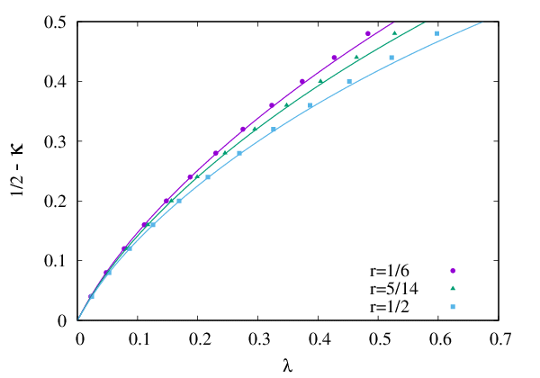
We note that, for large , the expression (34) simplifies because one can write
| (35) |
which leads to
| (36) |
and shows the correction to the linear term and its functional dependence on explicitly. In particular, the spectrum is nonanalytic around the centre, signalling the transition to a logarithmic density of states, which is responsible for the scaling of the entanglement.
5.2 Maximal eigenvalues
We now turn to the scaling of the maximal eigenvalues. For , the asymptotic limit is rather easy to obtain, since the corresponding eigenfunction has Gaussian form, see on the right of Fig. 1. Writing
| (37) |
inserting from (24) as well as
| (38) |
and extending the integration to , since the width of the Gaussian is , one can evaluate (37) to obtain
| (39) |
Up to corrections of order , the exponential function is equal to one. The asymptotic value therefore is
| (40) |
and lies between for and for . In Fig. 6, numerical data are shown and one sees that they approach this limit (from below, in accordance with (39)) as increases.
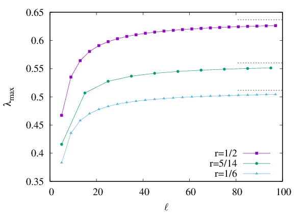

To obtain and the resulting is much more difficult. Calculating as the expectation value together with a continuum limit as in (37) gives an which is proportional to , but with incorrect prefactor. The reason has to be sought in the rapid oscillations of . We therefore present only numerical results on the right side of Fig. 6. They can be fitted with an ansatz as for the infinite case. The asymptotic value is given by the slope of these curves, which shows a slow increase with similarly to .
5.3 Relation between and
The difference between the matrix in the entanglement Hamiltonian and the commuting is completely due to their different spectra, see Fig. 2. Therefore, the first step in finding a general relation between both quantities, is to connect their spectra. In the infinite system, this was possible with the help of an asymptotic integral expression for which led to the formula [17]
| (41) |
with a generalized hypergeometric function .
For finite rings or chains, the numerics show clearly, that there is an analogous relation between these quantities which, however, depends on the ratio . This is demonstrated on the left of Fig. 7 for the half-ring with and compared to the infinite case .


On the right, the -dependence for the case is shown in more detail. One can see that, starting from an infinite system, decreases at first, but finally, close to the half-ring, becomes larger again. This holds in particular for the maximal values. As a consequence, the ratio of the hopping matrix elements also shows such a non-monotonous behaviour as a function of . Another consequence is that the scaling function for cannot have the simple form , but must depend on in a more complicated way.
In the infinite system, the asymptotic analysis of the eigenvalues was actually carried out by considering the reduced overlap kernel between the occupied momentum states via the equations [25]
| (42) |
but using a commuting differential operator to determine the eigenfunctions. This technique can not be applied in finite rings, since the momenta are discrete and is a matrix. In fact, for the half-filled half-ring it has exactly the same form as with and and the commuting quantity is again the matrix but with momentum indices. Therefore, one has to treat a discrete problem. There are analogues of WKB techniques for difference equations [29], but we have not pursued this.
6 Discussion
We have studied free fermions hopping on finite rings and open chains and determined the entanglement Hamiltonian from numerical calculations. This comprised the single-particle eigenvalue spectrum as well as the functional form in real space with the focus on half-filled systems. While these quantities depend on the aspect ratio , the main feature was the same as for subsystems in infinite systems: There is a difference between the properties of and the commuting operator which is the lattice analogue of the conformal entanglement Hamiltonian. We showed that such a does exist also for a subsystem at the end of an open chain and describe in the Appendix how to infer it for the transverse Ising model.
In contrast to the infinite case, the number of analytical results was limited, because the basic eigenvalue problem involves a finite matrix, and a simple continuum limit for the case of large subsystems is in general not sufficient. Even for , which is tridiagonal, the problem is complicated, since the matrix elements are trigonometric functions. Nevertheless we could find some analytical expressions for large for the small and large eigenvalues, but the general scaling function relating and , and therefore and , is still to be found.
In a broader context, the most intriguing feature is the existence of a simple commuting operator. The treatment in Section 3 shows the mechanism in a very transparent way. One can also prove [30] that a translationally invariant correlation matrix commuting with a tridiagonal matrix with simple spectrum must have the form (6). But does not seem to fit into the scheme of conserved quantities in the integrable spin models, and a physical explanation is still missing. One should also mention that if one uses in place of in the reduced density matrix, the resulting correlation function is not translationally invariant on a ring, although the deviations are rather small. One can say that a nonlinear relation between and , as found in the infinite case, is necessary to restore this symmetry
Appendix A Commuting operator for the TI chain
The transverse-field Ising model is known to be closely related to the XX chain which in turn is equivalent to the hopping model without site energies [31, 32, 33, 34]. This allows to find a commuting operator also for the TI chain without going through a separate calculation.
Consider a general open TI chain with Hamiltonian
| (43) |
In terms of fermions, this becomes
| (44) | |||||
and is diagonalized by a Bogoliubov transformation involving two functions and . They follow, together with the single-particle energies , from the coupled systems [35]
| (45) |
The eigenvalues come in pairs , and one can take e.g. the positive ones. Then the ground state is the fermionic vacuum and the correlation matrix combining and is given by
| (46) |
The entanglement Hamiltonian for a subsystem, which has again the form (44) but with matrices and , can then be found from the restricted correlation matrix and its transpose by solving the coupled systems
| (47) |
and constructing and from and the single-particle eigenvalues [24].
Now, it was pointed out in [23] that by writing (45) as a single system for the vector
| (48) |
the matrix in has the form
| (49) |
and thus is the same as for an inhomogeneous hopping model with sites and no site energies. The factor in (48) is included to have and all normalized to one. If the TI chain is homogeneous and critical, , is the same as in (2). Therefore has the form (4) with , and due to (46) and (48) the matrix and its transpose are submatrices of the correlation matrix of the hopping model [23]
| (50) |
where the minus sign appears because the ground state of the hopping model is half filled rather than empty.
Finally, considering the subsystem of the first sites in the hopping model and writing the eigenvectors of in analogy to (48) as
| (51) |
one sees that the equation , or , is equivalent to the system (47) and can be used to obtain . The commuting matrix , on the other hand, has the structure of in (49) with parameters
| (52) |
where the are given by (19) or (28) with and . Thus it describes a TI model on sites where couplings and fields increase towards the boundary and where the Hamiltonian commutes with .
The arguments used here are not restricted to the finite open chain, but hold also for rings or infinite systems (with proper handling of the boundary conditions). Thus in all these cases commuting operators follow from those of the half-filled hopping (XX) model.
References
References
- [1] Calabrese P, Cardy J and Doyon B 2009 Entanglement entropy in extended quantum systems J. Phys. A: Math. Theor. 42 500301
- [2] Laflorencie N 2016 Quantum entanglement in condensed matter systems Phys. Rep. 643 1
- [3] Li H and Haldane F D M 2008 Entanglement spectrum as a generalization of entanglement entropy: identification of topological order in non-abelian fractional quantum Hall effect states Phys. Rev. Lett. 101 010504
- [4] Casini H, Huerta M and Myers R C 2011 Towards a derivation of holographic entanglement entropy JHEP 05 036
- [5] Wong G, Klich I, Zayas L A P and Vaman D 2013 Entanglement temperature and entanglement entropy of excited states JHEP 12 020
- [6] Wen X, Ryu S and Ludwig A 2016 Evolution operators in conformal field theories and conformal mappings: entanglement Hamiltonian, the sine-square deformation, and others Phys. Rev. B 93 235119
- [7] Cardy J and Tonni E 2016 Entanglement Hamiltonians in two-dimensional conformal field theory J. Stat. Mech. P123103
- [8] Pretko M 2017 Nodal line entanglement entropy: Generalized Widom formula from entanglement Hamiltonians Phys. Rev. B 95 235111
- [9] Arias R E, Blanco D D, Casini H and Huerta M 2017 Local temperatures and local terms in modular Hamiltonians Phys. Rev. D 95 065005
- [10] Arias R E, Casini H, Huerta M and Pontello D 2017 Anisotropic Unruh temperatures Phys. Rev. D 96 105019
- [11] Klich I, Vaman D and Wong G 2017 Entanglement Hamiltonians for chiral fermions with zero modes Phys. Rev. Lett. 119 120401
- [12] Klich I, Vaman D and Wong G 2018 Entanglement Hamiltonians and entropy in 1+1D chiral fermion systems Phys. Rev. B 98 035134
- [13] Tonni E, Rodríguez-Laguna J and Sierra G 2018 Entanglement hamiltonian and entanglement contour in inhomogeneous 1D critical systems, J. Stat. Mech. 043105
- [14] Peschel I and Eisler V 2009 Reduced density matrices and entanglement entropy in free lattice models J. Phys. A: Math. Theor. 42 504003
- [15] Nienhuis B, Campostrini M and Calabrese P 2009 Entanglement, combinatorics and finite-size effects in spin-chains J. Stat. Mech. P02063
- [16] Kim P, Katsura H, Trivedi N and Han J H 2016 Entanglement and corner Hamiltonian spectra of integrable open spin chains Phys. Rev. B 94 195110
- [17] Eisler V and Peschel I 2017 Analytical results for the entanglement Hamiltonian of a free-fermion chain J. Phys. A: Math. Theor. 50 284003
- [18] Dalmonte M, Vermersch B and Zoller P 2018 Quantum Simulation and Spectroscopy of Entanglement Hamiltonians Nat. Phys. 14 827
- [19] Parisen Toldi F and Assaad F 2018 Entanglement Hamiltonian of interacting fermionic models, arXiv:1804.03163
- [20] Grünbaum F A 1981 Eigenvectors of a Toeplitz matrix: Discrete version of the prolate spheroidal wave functions SIAM J. Alg. Disc. Meth. 2 136
- [21] Xu W Y and Chamzas C 1984 On the periodic discrete prolate spheroidal sequences SIAM J. Appl. Math. 44 1210
- [22] Fagotti M and Calabrese P 2011 Universal parity effects in the entanglement entropy of XX chains with open boundary conditions J. Stat. Mech. P01017
- [23] Iglói F and Juhász R 2008 Exact relationship between the entanglement entropies of XY and quantum Ising chains EPL 81 57003
- [24] Peschel I 2003 Calculation of reduced density matrices from correlation functions J. Phys. A: Math. Gen. 36 L205
- [25] Eisler V and Peschel I 2013 Free-fermion entanglement and spheroidal functions J. Stat. Mech. P04028
- [26] Slepian D 1978 Prolate spheroidal wave functions, Fourier analysis, and uncertainty V: the discrete case Bell Syst. Techn. J. 57 1371
- [27] Peschel I 2004 On the reduced density matrix for a chain of free electrons J. Stat. Mech. P06004
- [28] Calabrese P and Cardy J 2004 Entanglement entropy and quantum field theory J. Stat. Mech. P06002
- [29] Dingle R B and Morgan G J 1968 WKB methods for difference equations Appl. Sci. Res. 18 221, 238
- [30] Grünbaum F A 1981 Toeplitz matrices commuting with tridiagonal matrices Lin. Alg. Appl. 40 25
- [31] Grady M 1982 Infinite set of conserved charges in the Ising model Phys. Rev. D 25 1103
- [32] Peschel I and Schotte K D 1984 Time correlations in quantum spin chains and the X-ray absorption problem Z. Physik B 54 305
- [33] Turban L 1984 Exactly solvable spin-1/2 quantum chains with multispin interactions Phys. Lett. 104 435
- [34] Iglói F, Juhász R and Rieger H 2000 Random antiferromagnetic quantum spin chains: Exact results from scaling of rare regions Phys. Rev. B 61 11552
- [35] Lieb E, Schultz T and Mattis D 1961 Two soluble models of an antiferromagnetic chain Ann. Phys. 16 407