跳到论文正文
W Papers独立论文阅读器 arXiv:1804.11222 论文正文 计算阅读时间 · 0%
引用这篇论文根据当前论文元数据生成,正式投稿前建议核对。


License: arXiv.org perpetual non-exclusive license
arXiv:1804.11222v4 [cs.LO] 20 Feb 2024

An optimized KE-tableau-based system for reasoning in the description logic \mathcal​D​L𝐃4,×\mathcal{DL}_{\mathbf{D}}^{4,\!\times} (Extended Version)

Domenico Cantone    Marianna Nicolosi-Asmundo    Daniele Francesco Santamaria Affiliation: University of Catania, Dept. of Mathematics and Computer Science
 email: {cantone,nicolosi,santamaria}@dmi.unict.it
Abstract

We present a KE-tableau-based procedure for the main TBox and ABox reasoning tasks for the description logic \mathcal​D​L​⟨𝟦​𝖫​𝖰​𝖲𝖱,×⟩​(𝐃)\mathcal{DL}\langle\mathsf{4LQS^{R,\!\times}}\rangle(\mathbf{D}), in short \mathcal​D​L𝐃4,×\mathcal{DL}_{\mathbf{D}}^{4,\!\times}. The logic \mathcal​D​L𝐃4,×\mathcal{DL}_{\mathbf{D}}^{4,\!\times}, representable in the decidable multi-sorted quantified set-theoretic fragment 𝟦​𝖫​𝖰​𝖲𝖱\mathsf{4LQS^{R}}, combines the high scalability and efficiency of rule languages such as the Semantic Web Rule Language (SWRL) with the expressivity of description logics.

Our algorithm is based on a variant of the KE-tableau system for sets of universally quantified clauses, where the KE-elimination rule is generalized in such a way as to incorporate the γ\gamma-rule. The novel system, called KEγ-tableau, turns out to be an improvement of the system introduced in [3] and of standard first-order KE-tableaux [11]. Suitable benchmark test sets executed on C++ implementations of the three mentioned systems show that the performances of the KEγ-tableau-based reasoner are often up to about 400% better than the ones of the other two systems. This a first step towards the construction of efficient reasoners for expressive OWL ontologies based on fragments of computable set-theory.

1 Introduction

Recently, decidability results in Computable Set Theory have been used for knowledge representation and reasoning, in particular, in the context of description logics (DLs) and rule languages for the Semantic Web. Such efforts are motivated by the fact that there exists a natural translation function between set-theoretical fragments and languages for the Semantic Web.

In particular, the decidable four-level stratified set-theoretic fragment 𝟦​𝖫​𝖰​𝖲𝖱\mathsf{4LQS^{R}}, involving variables of four sorts, pair terms, and a restricted form of quantification over variables of the first three sorts (cf. [1]) has been used in [2] to represent the DL \mathcal​D​L​⟨𝟦​𝖫​𝖰​𝖲𝖱,×⟩​(𝐃)\mathcal{DL}\langle\mathsf{4LQS^{R,\!\times}}\rangle(\mathbf{D}), in short \mathcal​D​L𝐃4,×\mathcal{DL}_{\mathbf{D}}^{4,\!\times}.

The DL \mathcal​D​L𝐃4,×\mathcal{DL}_{\mathbf{D}}^{4,\!\times} admits Boolean operations on concepts, concept domain and range, existential quantification, and minimum cardinality on the left-hand side of inclusion axioms. It also supports role constructs such as role chains on the left hand side of inclusion axioms, Boolean operations on (abstract and concrete) roles, product of concepts, and properties on roles such as transitivity, symmetry, reflexivity, and irreflexivity. The DL \mathcal​D​L𝐃4,×\mathcal{DL}_{\mathbf{D}}^{4,\!\times} admits also data types, a simple form of concrete domains that are relevant in real world applications. In addition, it permits to express the Semantic Web Rule Language (SWRL), an extension of the Ontology Web Language (OWL). Decidability of the Conjunctive Query Answering (CQA) problem for \mathcal​D​L𝐃4,×\mathcal{DL}_{\mathbf{D}}^{4,\!\times} has been proved in [2] via a reduction to the CQA problem for 𝟦​𝖫​𝖰​𝖲𝖱\mathsf{4LQS^{R}}, whose decidability easily follows from that of 𝟦​𝖫​𝖰​𝖲𝖱\mathsf{4LQS^{R}} (see [1]). In [2], the authors provided a terminating KE-tableau based procedure that, given a \mathcal​D​L𝐃4,×\mathcal{DL}_{\mathbf{D}}^{4,\!\times}-query QQ and a \mathcal​D​L𝐃4,×\mathcal{DL}_{\mathbf{D}}^{4,\!\times}-knowledge base \mathcal​K​B\mathcal{KB} represented in set-theoretic terms, determines the answer set of QQ with respect to \mathcal​K​B\mathcal{KB}. Notice that such an algorithm serves also as a decision procedure for the consistency problem for \mathcal​D​L𝐃4,×\mathcal{DL}_{\mathbf{D}}^{4,\!\times}-knowledge bases (KBs). We recall that KE-tableau systems [6] construct tableaux whose distinct branches define mutually exclusive situations, thus preventing the proliferation of redundant branches, typical of semantic tableaux.

The results presented in [2] have been extended in [3] to the main ABox reasoning tasks for \mathcal​D​L𝐃4,×\mathcal{DL}_{\mathbf{D}}^{4,\!\times}, such as instance checking and concept retrieval. by defining the Higher-Order Conjunctive Query Answering (HOCQA) problem for \mathcal​D​L𝐃4,×\mathcal{DL}_{\mathbf{D}}^{4,\!\times}. Such problem, instantiable to the principal reasoning tasks for \mathcal​D​L𝐃4,×\mathcal{DL}_{\mathbf{D}}^{4,\!\times}-ABoxes, has been defined by introducing Higher Order (HO) \mathcal​D​L𝐃4,×\mathcal{DL}_{\mathbf{D}}^{4,\!\times}-conjunctive queries, admitting variables of three sorts: individual and data type variables, concept variables, and role variables. Decidability of the HOCQA problem for \mathcal​D​L𝐃4,×\mathcal{DL}_{\mathbf{D}}^{4,\!\times} has been proved via a reduction to the HOCQA problem for the set-theoretic fragment 𝟦​𝖫​𝖰​𝖲𝖱\mathsf{4LQS^{R}}.

In [5], an implementation of the KE-tableau procedure defined in [3] has been presented. Such prototype, written in C++, supports OWL 2 \mathcal​D​L𝐃4,×\mathcal{DL}_{\mathbf{D}}^{4,\!\times}-KBs in the OWL/XML serialization. It was implemented only for TBox-reasoning services, namely, for verifying the consistency of given ontologies. Purely universal quantifiers are eliminated by the reasoner during a preprocessing phase, in which each quantified formula is instantiated in a systematic way with the individuals of the KB. The resulting instances are then suitably handled by applying the KE-elimination and bivalence rules. In the light of the benchmarking of the prototype, it turned out that the preprocessing phase of the universally quantified formulae is more and more expensive as the size of the KB grows.

In this paper, the KE-tableau-based procedure defined in [3] is modified, by eliminating the preprocessing phase for universally quantified formulae and replacing the standard KE-elimination rule with a novel elimination rule, called Eγ​-rule\textnormal{E}^{\gamma}\textnormal{-rule}, incorporating the standard rule for treating universally quantified formulae (γ\gamma-rule). The resulting system turns out to be more efficient than the KE-system in [5] and the First-Order (FO) KE-system in [11] as shown by suitable benchmarking tests executed on C++ implementations of the three systems. The main reason for such a speed-up relies on the fact that the novel Eγ​-rule\textnormal{E}^{\gamma}\textnormal{-rule} does not need to store the instances of universally quantified formulae on the KE-tableau.

2 Preliminaries

2.1 The set-theoretic fragment

It is convenient to recall the main set-theoretic notions behind the DL \mathcal​D​L𝐃4,×\mathcal{DL}_{\mathbf{D}}^{4,\!\times} and its reasoning problems. For space reasons, we refrain from reporting the syntax and semantics of the whole 𝟦​𝖫​𝖰​𝖲𝖱\mathsf{4LQS^{R}}, as the interested reader can find it in [1] together with the decision procedure for the satisfiability problem for 𝟦​𝖫​𝖰​𝖲𝖱\mathsf{4LQS^{R}}. Thus, we restrict our attention to the class of 𝟦​𝖫​𝖰​𝖲𝖱\mathsf{4LQS^{R}}-formulae actually involved in the set-theoretic representation of \mathcal​D​L𝐃4,×\mathcal{DL}_{\mathbf{D}}^{4,\!\times}, namely propositional combinations of 𝟦​𝖫​𝖰​𝖲𝖱\mathsf{4LQS^{R}}-quantifier-free literals (atomic formulae or their negations) and 𝟦​𝖫​𝖰​𝖲𝖱\mathsf{4LQS^{R}} purely universal formulae of the types displayed in Table 1. For the sake of conciseness we refer to such class of 𝟦​𝖫​𝖰​𝖲𝖱\mathsf{4LQS^{R}}-formulae as 𝟦​𝖫​𝖰​𝖲\mathcal​D​LD4,​×R\mathsf{4LQS}_{\scriptscriptstyle{\mathcal{DL}_{\lx@scalerel@obj{\mathbf{D}}}^{\lx@scalerel@obj{4,\!\times}}}}^{R}.

We recall that the fragment 𝟦​𝖫​𝖰​𝖲𝖱\mathsf{4LQS^{R}} admits four collections, 𝚅𝚊𝚛i\mathtt{Var}_{i}, of variables of sort ii, for i=0,1,2,3i=0,1,2,3. Variables of sort ii, for i=0,1,2,3i=0,1,2,3, are denoted by Xi,Yi,Zi,…X^{i},Y^{i},Z^{i},\ldots (in particular, variables of sort 00 are also denoted by x,y,z,…x,y,z,\ldots). In addition to variables, also pair terms of the form ⟨x,y⟩\langle x,y\rangle, with x,y∈𝚅𝚊𝚛0x,y\in\mathtt{Var}_{0} are allowed. Since the types of formulae illustrated in Table 1 do not involve variables of sort 22, notions and definitions concerning 𝟦​𝖫​𝖰​𝖲\mathcal​D​LD4,​×R\mathsf{4LQS}_{\scriptscriptstyle{\mathcal{DL}_{\lx@scalerel@obj{\mathbf{D}}}^{\lx@scalerel@obj{4,\!\times}}}}^{R}-formulae refer to variables of sorts 0,10,1, and 33 only.

Quantifier-free literals of level 0 Purely universal quantified formulae of level 1
x=y,x∈X1,⟨x,y⟩∈X3x=y,\;x\in X^{1},\;\langle x,y\rangle\in X^{3} (∀z1)​…​(∀zn)​φ0(\forall z_{1})\ldots(\forall z_{n})\varphi_{0}, where z1,…,zn∈𝚅𝚊𝚛0z_{1},\ldots,z_{n}\in\mathtt{Var}_{0} and φ0\varphi_{0} is any propositional combination of quantifier-free atomic formulae of level 0
¬(x=y),¬(x∈X1),¬(⟨x,y⟩∈X3)\neg(x=y),\;\neg(x\in X^{1}),\;\neg(\langle x,y\rangle\in X^{3})
Table 1: Types of literals and quantified formulae admitted in 𝟦​𝖫​𝖰​𝖲\mathcal​D​LD4,​×R\mathsf{4LQS}_{\scriptscriptstyle{\mathcal{DL}_{\lx@scalerel@obj{\mathbf{D}}}^{\lx@scalerel@obj{4,\!\times}}}}^{R}.

The variables z1,…,znz_{1},\ldots,z_{n} are said to occur quantified in (∀z1)​…​(∀zn)​φ0(\forall z_{1})\ldots(\forall z_{n})\varphi_{0}. A variable occurs free in a 𝟦​𝖫​𝖰​𝖲\mathcal​D​LD4,​×R\mathsf{4LQS}_{\scriptscriptstyle{\mathcal{DL}_{\lx@scalerel@obj{\mathbf{D}}}^{\lx@scalerel@obj{4,\!\times}}}}^{R}-formula φ\varphi if it does not occur quantified in any subformula of φ\varphi. For i=0,1,3i=0,1,3, we denote with 𝚅𝚊𝚛i​(φ)\mathtt{Var}_{i}(\varphi) the collections of variables of sort ii occurring free in φ\varphi.

Given sequences of distinct variables x→\vec{x} (in 𝚅𝚊𝚛0\mathtt{Var}_{0}), X→1\vec{X}^{1} (in 𝚅𝚊𝚛1\mathtt{Var}_{1}), and X→3\vec{X}^{3} (in 𝚅𝚊𝚛3\mathtt{Var}_{3}), of length nn, mm, and qq, respectively, and sequences of (not necessarily distinct) variables y→\vec{y} (in 𝚅𝚊𝚛0\mathtt{Var}_{0}), Y→1\vec{Y}^{1} (in 𝚅𝚊𝚛1\mathtt{Var}_{1}), and Y→3\vec{Y}^{3} (in 𝚅𝚊𝚛3\mathtt{Var}_{3}), also of length nn, mm, and qq, respectively, the 𝟦​𝖫​𝖰​𝖲\mathcal​D​LD4,​×R\mathsf{4LQS}_{\scriptscriptstyle{\mathcal{DL}_{\lx@scalerel@obj{\mathbf{D}}}^{\lx@scalerel@obj{4,\!\times}}}}^{R}-substitution σ≔{x→/y→,X→1/Y→1,X→3/Y→3}\sigma\coloneqq\{\vec{x}/\vec{y},\vec{X}^{1}/\vec{Y}^{1},\vec{X}^{3}/\vec{Y}^{3}\} is the mapping φ↦φ​σ\varphi\mapsto\varphi\sigma such that, for any given universal quantified 𝟦​𝖫​𝖰​𝖲\mathcal​D​LD4,​×R\mathsf{4LQS}_{\scriptscriptstyle{\mathcal{DL}_{\lx@scalerel@obj{\mathbf{D}}}^{\lx@scalerel@obj{4,\!\times}}}}^{R}-formula φ\varphi, φ​σ\varphi\sigma is the 𝟦​𝖫​𝖰​𝖲\mathcal​D​LD4,​×R\mathsf{4LQS}_{\scriptscriptstyle{\mathcal{DL}_{\lx@scalerel@obj{\mathbf{D}}}^{\lx@scalerel@obj{4,\!\times}}}}^{R}-formula obtained from φ\varphi by replacing the free occurrences of the variable xix_{i} in x→\vec{x} with the corresponding yiy_{i} in y→\vec{y} (for i=1,…,ni=1,\ldots,n), of Xj1X^{1}_{j} in X→1\vec{X}^{1} with Yj1Y^{1}_{j} in Y→1\vec{Y}^{1} (for j=1,…,mj=1,\ldots,m), and of Xh3X^{3}_{h} in X→3\vec{X}^{3} with Yh3Y^{3}_{h} in Y→3\vec{Y}^{3} (for h=1,…,qh=1,\ldots,q), respectively. A substitution σ\sigma is free for φ\varphi if the formulae φ\varphi and φ​σ\varphi\sigma have exactly the same occurrences of quantified variables. The empty substitution, denoted by ϵ\epsilon, satisfies φ​ϵ=φ\varphi\epsilon=\varphi, for each 𝟦​𝖫​𝖰​𝖲\mathcal​D​LD4,​×R\mathsf{4LQS}_{\scriptscriptstyle{\mathcal{DL}_{\lx@scalerel@obj{\mathbf{D}}}^{\lx@scalerel@obj{4,\!\times}}}}^{R}-formula φ\varphi.

A 𝟦​𝖫​𝖰​𝖲\mathcal​D​LD4,​×R\mathsf{4LQS}_{\scriptscriptstyle{\mathcal{DL}_{\lx@scalerel@obj{\mathbf{D}}}^{\lx@scalerel@obj{4,\!\times}}}}^{R}-interpretation is a pair ℳ=(𝒟,ℳ)\mathbfcal{M}=(D,M), where DD is a nonempty collection of objects (called domain or universe of ℳ\mathbfcal{M}) and MM is an assignment over the variables in \mathcal​Vi\mathcal{V}_{i}, for i=0,1,3i=0,1,3, such that: M​X0∈D,M​X1∈\mathcal​P​(D)MX^{0}\in D,MX^{1}\in\mathcal{P}(D), and M​X3∈\mathcal​P​(\mathcal​P​(\mathcal​P​(D)))MX^{3}\in\mathcal{P}(\mathcal{P}(\mathcal{P}(D))), where Xi∈\mathcal​ViX^{i}\in\mathcal{V}_{i}, for i=0,1,3i=0,1,3, and \mathcal​P​(s)\mathcal{P}(s) denotes the powerset of ss.

Pair terms are interpreted à la Kuratowski, and therefore we put

M⁡⟨x,y⟩≔{{M​x},{M​x,M​y}}M\langle x,y\rangle\coloneqq\{\{Mx\},\{Mx,My\}\}.

Next, let

  • -

    ℳ=(𝒟,ℳ)\mathbfcal{M}=(D,M) be a 𝟦​𝖫​𝖰​𝖲\mathcal​D​LD4,​×R\mathsf{4LQS}_{\scriptscriptstyle{\mathcal{DL}_{\lx@scalerel@obj{\mathbf{D}}}^{\lx@scalerel@obj{4,\!\times}}}}^{R}-interpretation,

  • -

    x1,…,xn∈\mathcal​V0x_{1},\ldots,x_{n}\in\mathcal{V}_{0}, and

  • -

    u1,…,un∈Du_{1},\ldots,u_{n}\in D.

By ℳ⁡[§→/⊓→]\mathbfcal{M}[\vec{x}/\vec{u}], we denote the interpretation ℳ′=(𝒟,ℳ′)\mathbfcal{M}^{\prime}=(D,M^{\prime}) such that M′​xi=uiM^{\prime}x_{i}=u_{i} (for i=1,…,ni=1,\ldots,n). For a 𝟦​𝖫​𝖰​𝖲\mathcal​D​LD4,​×R\mathsf{4LQS}_{\scriptscriptstyle{\mathcal{DL}_{\lx@scalerel@obj{\mathbf{D}}}^{\lx@scalerel@obj{4,\!\times}}}}^{R}-interpretation ℳ=(𝒟,ℳ)\mathbfcal{M}=(D,M) and a 𝟦​𝖫​𝖰​𝖲\mathcal​D​LD4,​×R\mathsf{4LQS}_{\scriptscriptstyle{\mathcal{DL}_{\lx@scalerel@obj{\mathbf{D}}}^{\lx@scalerel@obj{4,\!\times}}}}^{R}-formula φ\varphi, the satisfiability relationship ℳ⊧φ\mathbfcal{M}\models\varphi is recursively defined over the structure of φ\varphi as follows. Quantifier-free literals are evaluated in a standard way according to the usual meaning of the predicates ‘∈\in’ and ‘==’, and of the propositional negation ‘¬\neg’. Purely universal formulae are evaluated as follows:

ℳ⊧(∀‡∞)…(∀‡\)φ′\mathbfcal{M}\models(\forall z_{1})\ldots(\forall z_{n})\varphi_{0}  iff  ℳ⁡[‡→/⊓→]⊧φ′\mathbfcal{M}[\vec{z}/\vec{u}]\models\varphi_{0}, for all u→∈Dn\vec{u}\in D^{n}.

Finally, compound formulae are interpreted according to the standard rules of propositional logic. If ℳ⊧φ\mathbfcal{M}\models\varphi, then ℳ\mathbfcal{M} is said to be a 𝟦​𝖫​𝖰​𝖲\mathcal​D​LD4,​×R\mathsf{4LQS}_{\scriptscriptstyle{\mathcal{DL}_{\lx@scalerel@obj{\mathbf{D}}}^{\lx@scalerel@obj{4,\!\times}}}}^{R}-model for φ\varphi. A 𝟦​𝖫​𝖰​𝖲\mathcal​D​LD4,​×R\mathsf{4LQS}_{\scriptscriptstyle{\mathcal{DL}_{\lx@scalerel@obj{\mathbf{D}}}^{\lx@scalerel@obj{4,\!\times}}}}^{R}-formula is said to be satisfiable if it has a 𝟦​𝖫​𝖰​𝖲\mathcal​D​LD4,​×R\mathsf{4LQS}_{\scriptscriptstyle{\mathcal{DL}_{\lx@scalerel@obj{\mathbf{D}}}^{\lx@scalerel@obj{4,\!\times}}}}^{R}-model. A 𝟦​𝖫​𝖰​𝖲\mathcal​D​LD4,​×R\mathsf{4LQS}_{\scriptscriptstyle{\mathcal{DL}_{\lx@scalerel@obj{\mathbf{D}}}^{\lx@scalerel@obj{4,\!\times}}}}^{R}-formula is valid if it is satisfied by all 𝟦​𝖫​𝖰​𝖲\mathcal​D​LD4,​×R\mathsf{4LQS}_{\scriptscriptstyle{\mathcal{DL}_{\lx@scalerel@obj{\mathbf{D}}}^{\lx@scalerel@obj{4,\!\times}}}}^{R}-interpretations.

2.2 The logic \mathcal​D​L​⟨𝟦​𝖫​𝖰​𝖲𝖱,×⟩​(𝐃)\mathcal{DL}\langle\mathsf{4LQS^{R,\!\times}}\rangle(\mathbf{D})

In what follows we introduce the syntax and the semantics of the DL \mathcal​D​L​⟨𝟦​𝖫​𝖰​𝖲𝖱,×⟩​(𝐃)\mathcal{DL}\langle\mathsf{4LQS^{R,\!\times}}\rangle(\mathbf{D}) (as remarked above, more simply referred to as \mathcal​D​L𝐃4,×\mathcal{DL}_{\mathbf{D}}^{4,\!\times}).

Let 𝐑𝐀\mathbf{R_{A}}, 𝐑𝐃\mathbf{R_{D}}, 𝐂\mathbf{C}, 𝐈\mathbf{I} be denumerable pairwise disjoint sets of abstract role names, concrete role names, concept names, and individual names, respectively.

Definition of data types relies on the notion of data type map, given according to [12] as follows. Let 𝐃=(ND,NC,NF,⋅𝐃)\mathbf{D}=(N_{D},N_{C},N_{F},\cdot^{\mathbf{D}}) be a data type map, where NDN_{D} is a finite set of data types, NCN_{C} is a function assigning a set of constants NC​(d)N_{C}(d) to each data type d∈NDd\in N_{D}, NFN_{F} is a function assigning a set of facets NF​(d)N_{F}(d) to each d∈NDd\in N_{D}, and ⋅𝐃\cdot^{\mathbf{D}} is a function assigning a data type interpretation d𝐃d^{\mathbf{D}} to each d∈NDd\in N_{D}, a facet interpretation f𝐃⊆d𝐃f^{\mathbf{D}}\subseteq d^{\mathbf{D}} to each facet f∈NF​(d)f\in N_{F}(d), and a data value ed𝐃∈d𝐃e_{d}^{\mathbf{D}}\in d^{\mathbf{D}} to every constant ed∈NC​(d)e_{d}\in N_{C}(d). We shall assume that the interpretations of the data types in NDN_{D} are nonempty pairwise disjoint sets.

(a) \mathcal​D​L𝐃4,×\mathcal{DL}_{\mathbf{D}}^{4,\!\times}-data type, (b) \mathcal​D​L𝐃4,×\mathcal{DL}_{\mathbf{D}}^{4,\!\times}-concept, (c) \mathcal​D​L𝐃4,×\mathcal{DL}_{\mathbf{D}}^{4,\!\times}-abstract role, and (d) \mathcal​D​L𝐃4,×\mathcal{DL}_{\mathbf{D}}^{4,\!\times}-concrete role terms are constructed according to the following syntax rules:

  • (a)

    t1,t2⟶d​r​|¬t1|​t1⊓t2​|t1⊔t2|​{ed},t_{1},t_{2}\longrightarrow dr~|~\neg t_{1}~|~t_{1}\sqcap t_{2}~|~t_{1}\sqcup t_{2}~|~\{e_{d}\}\,,

  • (b)

    C1,C2⟶A|⊤|⊥|¬C1|C1⊔C2|C1⊓C2|{a}|∃R.𝑆𝑒𝑙𝑓|∃R.{a}|∃P.{ed},C_{1},C_{2}\longrightarrow A~|~\top~|~\bot~|~\neg C_{1}~|~C_{1}\sqcup C_{2}~|~C_{1}\sqcap C_{2}~|~\{a\}~|~\exists R.\mathit{Self}|\exists R.\{a\}|\exists P.\{e_{d}\}\,,

  • (c)

    R1,R2⟶S|U|R1−1|¬R1|R1⊔R2|R1⊓R2|RC1||R|C1|RC1|C2|id(C)|R_{1},R_{2}\longrightarrow S~|~U~|~R_{1}^{-1}~|~\neg R_{1}~|~R_{1}\sqcup R_{2}~|~R_{1}\sqcap R_{2}~|~R_{C_{1}|}~|~R_{|C_{1}}~|~R_{C_{1}~|~C_{2}}~|~id(C)~|~

    C1×C2,C_{1}\times C_{2}\,,

  • (d)

    P1,P2⟶T|¬P1|P1⊔P2|P1⊓P2|PC1||P|t1|PC1|t1,P_{1},P_{2}\longrightarrow T~|~\neg P_{1}~|~P_{1}\sqcup P_{2}~|~P_{1}\sqcap P_{2}~|~P_{C_{1}|}~|~P_{|t_{1}}~|~P_{C_{1}|t_{1}}\,,

where d​rdr is a data range for 𝐃\mathbf{D}, t1,t2t_{1},t_{2} are data type terms, ede_{d} is a constant in NC​(d)N_{C}(d), aa is an individual name, AA is a concept name, C1,C2C_{1},C_{2} are \mathcal​D​L𝐃4,×\mathcal{DL}_{\mathbf{D}}^{4,\!\times}-concept terms, SS is an abstract role name, UU is an abstract role name denoting the universal role, R,R1,R2R,R_{1},R_{2} are \mathcal​D​L𝐃4,×\mathcal{DL}_{\mathbf{D}}^{4,\!\times}-abstract role terms, TT is a concrete role name, and P,P1,P2P,P_{1},P_{2} are \mathcal​D​L𝐃4,×\mathcal{DL}_{\mathbf{D}}^{4,\!\times}-concrete role terms. We remark that data type terms are introduced in order to represent derived data types.

A \mathcal​D​L𝐃4,×\mathcal{DL}_{\mathbf{D}}^{4,\!\times}-KB is a triple \mathcal​K=(\mathcal​R,\mathcal​T,\mathcal​A){\mathcal K}=(\mathcal{R},\mathcal{T},\mathcal{A}) such that \mathcal​R\mathcal{R} is a \mathcal​D​L𝐃4,×\mathcal{DL}_{\mathbf{D}}^{4,\!\times}-R​B​o​xRBox, \mathcal​T\mathcal{T} is a \mathcal​D​L𝐃4,×\mathcal{DL}_{\mathbf{D}}^{4,\!\times}-T​B​o​xTBox, and \mathcal​A\mathcal{A} a \mathcal​D​L𝐃4,×\mathcal{DL}_{\mathbf{D}}^{4,\!\times}-A​B​o​xABox.

A \mathcal​D​L𝐃4,×\mathcal{DL}_{\mathbf{D}}^{4,\!\times}-R​B​o​xRBox is a collection of statements of the following forms:

R1≡R2,R1⊑R2,R1​…​Rn⊑Rn+1,𝖲𝗒𝗆⁡(R1),𝖠𝗌𝗒𝗆⁡(R1),𝖱𝖾𝖿⁡(R1),𝖨𝗋𝗋𝖾𝖿⁡(R1),𝖣𝗂𝗌⁡(R1,R2),𝖳𝗋𝖺⁡(R1),𝖥𝗎𝗇⁡(R1),R1≡C1×C2,P1≡P2,P1⊑P2,𝖣𝗂𝗌⁡(P1,P2),𝖥𝗎𝗇⁡(P1),\begin{array}[]{cccccccccc}R_{1}\equiv R_{2},&R_{1}\sqsubseteq R_{2},&~~R_{1}\ldots R_{n}\sqsubseteq R_{n+1}~~,&\mathsf{Sym}(R_{1}),&\mathsf{Asym}(R_{1}),\\ \mathsf{Ref}(R_{1}),&\mathsf{Irref}(R_{1}),&\mathsf{Dis}(R_{1},R_{2}),&\mathsf{Tra}(R_{1}),&\mathsf{Fun}(R_{1}),\\ R_{1}\equiv C_{1}\times C_{2},&P_{1}\equiv P_{2},&P_{1}\sqsubseteq P_{2},&\mathsf{Dis}(P_{1},P_{2}),&\mathsf{Fun}(P_{1}),\end{array}

where R1,R2R_{1},R_{2} are \mathcal​D​L𝐃4,×\mathcal{DL}_{\mathbf{D}}^{4,\!\times}-abstract role terms, C1,C2C_{1},C_{2} are \mathcal​D​L𝐃4,×\mathcal{DL}_{\mathbf{D}}^{4,\!\times}-abstract concept terms, and P1,P2P_{1},P_{2} are \mathcal​D​L𝐃4,×\mathcal{DL}_{\mathbf{D}}^{4,\!\times}-concrete role terms. Any expression of the type w⊑Rw\sqsubseteq R, where ww is a finite string of \mathcal​D​L𝐃4,×\mathcal{DL}_{\mathbf{D}}^{4,\!\times}-abstract role terms and RR is an \mathcal​D​L𝐃4,×\mathcal{DL}_{\mathbf{D}}^{4,\!\times}-abstract role term, is called a role inclusion axiom (RIA).

A \mathcal​D​L𝐃4,×\mathcal{DL}_{\mathbf{D}}^{4,\!\times}-T​B​o​xTBox is a set of statements of the types:

  • -

    C1≡C2C_{1}\equiv C_{2}, C1⊑C2C_{1}\sqsubseteq C_{2}, C1⊑∀R1.C2C_{1}\sqsubseteq\forall R_{1}.C_{2}, ∃R1.C1⊑C2\exists R_{1}.C_{1}\sqsubseteq C_{2}, ≥nR1.C1⊑C2\geq_{n}\!\!R_{1}.C_{1}\sqsubseteq C_{2},
    C1⊑≤nR1.C2C_{1}\sqsubseteq{\leq_{n}\!\!R_{1}.C_{2}},

  • -

    t1≡t2t_{1}\equiv t_{2}, t1⊑t2t_{1}\sqsubseteq t_{2}, C1⊑∀P1.t1C_{1}\sqsubseteq\forall P_{1}.t_{1}, ∃P1.t1⊑C1\exists P_{1}.t_{1}\sqsubseteq C_{1}, ≥nP1.t1⊑C1\geq_{n}\!\!P_{1}.t_{1}\sqsubseteq C_{1}, C1⊑≤nP1.t1C_{1}\sqsubseteq{\leq_{n}\!\!P_{1}.t_{1}},

where C1,C2C_{1},C_{2} are \mathcal​D​L𝐃4,×\mathcal{DL}_{\mathbf{D}}^{4,\!\times}-concept terms, t1,t2t_{1},t_{2} data type terms, R1R_{1} a \mathcal​D​L𝐃4,×\mathcal{DL}_{\mathbf{D}}^{4,\!\times}-abstract role term, P1P_{1} a \mathcal​D​L𝐃4,×\mathcal{DL}_{\mathbf{D}}^{4,\!\times}-concrete role term. Any statement of the form C⊑DC\sqsubseteq D, with CC, DD \mathcal​D​L𝐃4\mathcal{DL}_{\mathbf{D}}^{4}-concept terms, is a general concept inclusion axiom.

A \mathcal​D​L𝐃4,×\mathcal{DL}_{\mathbf{D}}^{4,\!\times}-A​B​o​xABox is a set of individual assertions of the forms: a:C1a:C_{1}, (a,b):R1(a,b):R_{1}, a=ba=b, a≠ba\neq b, ed:t1e_{d}:t_{1}, (a,ed):P1(a,e_{d}):P_{1}, with C1C_{1} a \mathcal​D​L𝐃4,×\mathcal{DL}_{\mathbf{D}}^{4,\!\times}-concept term, dd a data type, t1t_{1} a data type term, R1R_{1} a \mathcal​D​L𝐃4,×\mathcal{DL}_{\mathbf{D}}^{4,\!\times}-abstract role term, P1P_{1} a \mathcal​D​L𝐃4,×\mathcal{DL}_{\mathbf{D}}^{4,\!\times}-concrete role term, a,ba,b individual names, and ede_{d} a constant in NC​(d)N_{C}(d).

The semantics of \mathcal​D​L𝐃4,×\mathcal{DL}_{\mathbf{D}}^{4,\!\times} is given by means of an interpretation 𝐈=(Δ𝐈,Δ𝐃,⋅𝐈)\mathbf{I}=(\Delta^{\mathbf{I}},\Delta_{\mathbf{D}},\cdot^{\mathbf{I}}), where Δ𝐈\Delta^{\mathbf{I}} and Δ𝐃\Delta_{\mathbf{D}} are non-empty disjoint domains such that d𝐃⊆Δ𝐃d^{\mathbf{D}}\subseteq\Delta_{\mathbf{D}}, for every d∈NDd\in N_{D}, and ⋅𝐈\cdot^{\mathbf{I}} is an interpretation function. The definition of the interpretation of concepts and roles, axioms, and assertions is shown in Table 2.

Table 2: *
Name Syntax Semantics
concept AA A𝐈⊆Δ𝐈A^{\mathbf{I}}\subseteq\Delta^{\mathbf{I}}
ab. (resp., cn.) rl. RR (resp., PP ) R𝐈⊆Δ𝐈×Δ𝐈R^{\mathbf{I}}\subseteq\Delta^{\mathbf{I}}\times\Delta^{\mathbf{I}}    (resp., P𝐈⊆Δ𝐈×Δ𝐃P^{\mathbf{I}}\subseteq\Delta^{\mathbf{I}}\times\Delta_{\mathbf{D}})
individual aa a𝐈∈Δ𝐈a^{\mathbf{I}}\in\Delta^{\mathbf{I}}
nominal {a}\{a\} {a}𝐈={a𝐈}\{a\}^{\mathbf{I}}=\{a^{\mathbf{I}}\}
dtype (resp., ng.) dd (resp., ¬d\neg d) d𝐃⊆Δ𝐃d^{\mathbf{D}}\subseteq\Delta_{\mathbf{D}} (resp., Δ𝐃∖d𝐃\Delta_{\mathbf{D}}\setminus d^{\mathbf{D}})
negative data type term ¬t1\neg t_{1} (¬t1)𝐃=Δ𝐃∖t1𝐃(\neg t_{1})^{\mathbf{D}}=\Delta_{\mathbf{D}}\setminus t_{1}^{\mathbf{D}}
data type terms intersection t1⊓t2t_{1}\sqcap t_{2} (t1⊓t2)𝐃=t1𝐃∩t2𝐃(t_{1}\sqcap t_{2})^{\mathbf{D}}=t_{1}^{\mathbf{D}}\cap t_{2}^{\mathbf{D}}
data type terms union t1⊔t2t_{1}\sqcup t_{2} (t1⊔t2)𝐃=t1𝐃∪t2𝐃(t_{1}\sqcup t_{2})^{\mathbf{D}}=t_{1}^{\mathbf{D}}\cup t_{2}^{\mathbf{D}}
constant in NC​(d)N_{C}(d) ede_{d} ed𝐃∈d𝐃e_{d}^{\mathbf{D}}\in d^{\mathbf{D}}
data range {ed1,…,edn}\{e_{d_{1}},\ldots,e_{d_{n}}\} {ed1,…,edn}𝐃={ed1𝐃}∪…∪{edn𝐃}\{e_{d_{1}},\ldots,e_{d_{n}}\}^{\mathbf{D}}=\{e_{d_{1}}^{\mathbf{D}}\}\cup\ldots\cup\{e_{d_{n}}^{\mathbf{D}}\}
data range ψd\psi_{d} ψd𝐃\psi_{d}^{\mathbf{D}}
data range ¬d​r\neg dr Δ𝐃∖d​r𝐃\Delta_{\mathbf{D}}\setminus dr^{\mathbf{D}}
top (resp., bot.) ⊤\top (resp., ⊥\bot ) Δ𝐈\Delta^{\mathbf{I}} (resp., ∅\emptyset)
negation ¬C\neg C (¬C)𝐈=Δ𝐈∖C(\neg C)^{\mathbf{I}}=\Delta^{\mathbf{I}}\setminus C
conj. (resp., disj.) C⊓DC\sqcap D (resp., C⊔DC\sqcup D) (C⊓D)𝐈=C𝐈∩D𝐈(C\sqcap D)^{\mathbf{I}}=C^{\mathbf{I}}\cap D^{\mathbf{I}} (resp., (C⊔D)𝐈=C𝐈∪D𝐈(C\sqcup D)^{\mathbf{I}}=C^{\mathbf{I}}\cup D^{\mathbf{I}})
valued exist. quantification ∃R.a\exists R.{a} (∃R.a)𝐈={x∈Δ𝐈:⟨x,a𝐈⟩∈R𝐈}(\exists R.{a})^{\mathbf{I}}=\{x\in\Delta^{\mathbf{I}}:\langle x,a^{\mathbf{I}}\rangle\in R^{\mathbf{I}}\}
data typed exist. quantif. ∃P.ed\exists P.{e_{d}} (∃P.ed)𝐈={x∈Δ𝐈:⟨x,ed𝐃⟩∈P𝐈}(\exists P.e_{d})^{\mathbf{I}}=\{x\in\Delta^{\mathbf{I}}:\langle x,e^{\mathbf{D}}_{d}\rangle\in P^{\mathbf{I}}\}
self concept ∃R.𝑆𝑒𝑙𝑓\exists R.\mathit{Self} (∃R.𝑆𝑒𝑙𝑓)𝐈={x∈Δ𝐈:⟨x,x⟩∈R𝐈}(\exists R.\mathit{Self})^{\mathbf{I}}=\{x\in\Delta^{\mathbf{I}}:\langle x,x\rangle\in R^{\mathbf{I}}\}
nominals {a1,…,an}\{a_{1},\ldots,a_{n}\} {a1,…,an}𝐈={a1𝐈}∪…∪{an𝐈}\{a_{1},\ldots,a_{n}\}^{\mathbf{I}}=\{a_{1}^{\mathbf{I}}\}\cup\ldots\cup\{a_{n}^{\mathbf{I}}\}
universal role U (U)𝐈=Δ𝐈×Δ𝐈(U)^{\mathbf{I}}=\Delta^{\mathbf{I}}\times\Delta^{\mathbf{I}}
inverse role R−R^{-} (R−)𝐈={⟨y,x⟩∣⟨x,y⟩∈R𝐈}(R^{-})^{\mathbf{I}}=\{\langle y,x\rangle\mid\langle x,y\rangle\in R^{\mathbf{I}}\}
concept cart. prod. C1×C2C_{1}\times C_{2} (C1×C2)I=C1I×C2I(C_{1}\times C_{2})^{I}=C_{1}^{I}\times C_{2}^{I}
abstract role complement ¬R\neg R (¬R)𝐈=(Δ𝐈×Δ𝐈)∖R𝐈(\neg R)^{\mathbf{I}}=(\Delta^{\mathbf{I}}\times\Delta^{\mathbf{I}})\setminus R^{\mathbf{I}}
abstract role union R1⊔R2R_{1}\sqcup R_{2} (R1⊔R2)𝐈=R1𝐈∪R2𝐈(R_{1}\sqcup R_{2})^{\mathbf{I}}=R_{1}^{\mathbf{I}}\cup R_{2}^{\mathbf{I}}
abstract role intersection R1⊓R2R_{1}\sqcap R_{2} (R1⊓R2)𝐈=R1𝐈∩R2𝐈(R_{1}\sqcap R_{2})^{\mathbf{I}}=R_{1}^{\mathbf{I}}\cap R_{2}^{\mathbf{I}}
abstract role domain restr. RC∣R_{C\mid} (RC∣)𝐈={⟨x,y⟩∈R𝐈:x∈C𝐈}(R_{C\mid})^{\mathbf{I}}=\{\langle x,y\rangle\in R^{\mathbf{I}}:x\in C^{\mathbf{I}}\}
concrete role complement ¬P\neg P (¬P)𝐈=(Δ𝐈×Δ𝐃)∖P𝐈(\neg P)^{\mathbf{I}}=(\Delta^{\mathbf{I}}\times\Delta^{\mathbf{D}})\setminus P^{\mathbf{I}}
concrete role union P1⊔P2P_{1}\sqcup P_{2} (P1⊔P2)𝐈=P1𝐈∪P2𝐈(P_{1}\sqcup P_{2})^{\mathbf{I}}=P_{1}^{\mathbf{I}}\cup P_{2}^{\mathbf{I}}
concrete role intersection P1⊓P2P_{1}\sqcap P_{2} (P1⊓P2)𝐈=P1𝐈∩P2𝐈(P_{1}\sqcap P_{2})^{\mathbf{I}}=P_{1}^{\mathbf{I}}\cap P_{2}^{\mathbf{I}}
concrete role domain restr. PC∣P_{C\mid} (PC∣)𝐈={⟨x,y⟩∈P𝐈:x∈C𝐈}(P_{C\mid})^{\mathbf{I}}=\{\langle x,y\rangle\in P^{\mathbf{I}}:x\in C^{\mathbf{I}}\}
concrete role range restr. P∣tP_{\mid t} (P∣t)𝐈={⟨x,y⟩∈P𝐈:y∈t𝐃}(P_{\mid t})^{\mathbf{I}}=\{\langle x,y\rangle\in P^{\mathbf{I}}:y\in t^{\mathbf{D}}\}
concrete role restriction PC1|tP_{C_{1}\mid t} (PC1|t)𝐈={⟨x,y⟩∈P𝐈:x∈C1𝐈∧y∈t𝐃}(P_{C_{1}\mid t})^{\mathbf{I}}=\{\langle x,y\rangle\in P^{\mathbf{I}}:x\in C_{1}^{\mathbf{I}}\wedge y\in t^{\mathbf{D}}\}
concept subsum. C1⊑C2C_{1}\sqsubseteq C_{2} 𝐈⊧𝐃C1⊑C2⟺C1𝐈⊆C2𝐈\mathbf{I}\models_{\mathbf{D}}C_{1}\sqsubseteq C_{2}\;\Longleftrightarrow\;C_{1}^{\mathbf{I}}\subseteq C_{2}^{\mathbf{I}}
ab. role subsum. R1⊑R2R_{1}\sqsubseteq R_{2} 𝐈⊧𝐃R1⊑R2⟺R1𝐈⊆R2𝐈\mathbf{I}\models_{\mathbf{D}}R_{1}\sqsubseteq R_{2}\;\Longleftrightarrow\;R_{1}^{\mathbf{I}}\subseteq R_{2}^{\mathbf{I}}
role incl. axiom R1​…​Rn⊑RR_{1}\ldots R_{n}\sqsubseteq R 𝐈⊧𝐃R1…Rn⊑R⟺R1𝐈∘…∘Rn𝐈⊆R𝐈\mathbf{I}\models_{\mathbf{D}}R_{1}\ldots R_{n}\sqsubseteq R\;\Longleftrightarrow\;R_{1}^{\mathbf{I}}\circ\ldots\circ R_{n}^{\mathbf{I}}\subseteq R^{\mathbf{I}}
cn. role subsum. P1⊑P2P_{1}\sqsubseteq P_{2} 𝐈⊧𝐃P1⊑P2⟺P1𝐈⊆P2𝐈\mathbf{I}\models_{\mathbf{D}}P_{1}\sqsubseteq P_{2}\;\Longleftrightarrow\;P_{1}^{\mathbf{I}}\subseteq P_{2}^{\mathbf{I}}
symmetric role 𝖲𝗒𝗆⁡(R)\mathsf{Sym}(R) 𝐈⊧𝐃𝖲𝗒𝗆(R)⟺(R−)𝐈⊆R𝐈\mathbf{I}\models_{\mathbf{D}}\mathsf{Sym}(R)\;\Longleftrightarrow\;(R^{-})^{\mathbf{I}}\subseteq R^{\mathbf{I}}
asymmetric role 𝖠𝗌𝗒𝗆⁡(R)\mathsf{Asym}(R) 𝐈⊧𝐃𝖠𝗌𝗒𝗆(R)⟺R𝐈∩(R−)𝐈=∅\mathbf{I}\models_{\mathbf{D}}\mathsf{Asym}(R)\;\Longleftrightarrow\;R^{\mathbf{I}}\cap(R^{-})^{\mathbf{I}}=\emptyset
transitive role 𝖳𝗋𝖺⁡(R)\mathsf{Tra}(R) 𝐈⊧𝐃𝖳𝗋𝖺(R)⟺R𝐈∘R𝐈⊆R𝐈\mathbf{I}\models_{\mathbf{D}}\mathsf{Tra}(R)\;\Longleftrightarrow\;R^{\mathbf{I}}\circ R^{\mathbf{I}}\subseteq R^{\mathbf{I}}
disj. ab. role 𝖣𝗂𝗌⁡(R1,R2)\mathsf{Dis}(R_{1},R_{2}) 𝐈⊧𝐃𝖣𝗂𝗌(R1,R2)⟺R1𝐈∩R2𝐈=∅\mathbf{I}\models_{\mathbf{D}}\mathsf{Dis}(R_{1},R_{2})\;\Longleftrightarrow\;R_{1}^{\mathbf{I}}\cap R_{2}^{\mathbf{I}}=\emptyset
reflexive role 𝖱𝖾𝖿⁡(R)\mathsf{Ref}(R) 𝐈⊧𝐃𝖱𝖾𝖿(R)⟺{⟨x,x⟩∣x∈Δ𝐈}⊆R𝐈\mathbf{I}\models_{\mathbf{D}}\mathsf{Ref}(R)\;\Longleftrightarrow\;\{\langle x,x\rangle\mid x\in\Delta^{\mathbf{I}}\}\subseteq R^{\mathbf{I}}
irreflexive role 𝖨𝗋𝗋𝖾𝖿⁡(R)\mathsf{Irref}(R) 𝐈⊧𝐃𝖨𝗋𝗋𝖾𝖿(R)⟺R𝐈∩{⟨x,x⟩∣x∈Δ𝐈}=∅\mathbf{I}\models_{\mathbf{D}}\mathsf{Irref}(R)\;\Longleftrightarrow\;R^{\mathbf{I}}\cap\{\langle x,x\rangle\mid x\in\Delta^{\mathbf{I}}\}=\emptyset
func. ab. role 𝖥𝗎𝗇⁡(R)\mathsf{Fun}(R) 𝐈⊧𝐃𝖥𝗎𝗇(R)⟺(R−)𝐈∘R𝐈⊆{⟨x,x⟩∣x∈Δ𝐈}\mathbf{I}\models_{\mathbf{D}}\mathsf{Fun}(R)\;\Longleftrightarrow\;(R^{-})^{\mathbf{I}}\circ R^{\mathbf{I}}\subseteq\{\langle x,x\rangle\mid x\in\Delta^{\mathbf{I}}\}
disj. cn. role 𝖣𝗂𝗌⁡(P1,P2)\mathsf{Dis}(P_{1},P_{2}) 𝐈⊧𝐃𝖣𝗂𝗌(P1,P2)⟺P1𝐈∩P2𝐈=∅\mathbf{I}\models_{\mathbf{D}}\mathsf{Dis}(P_{1},P_{2})\;\Longleftrightarrow\;P_{1}^{\mathbf{I}}\cap P_{2}^{\mathbf{I}}=\emptyset
func. cn. role 𝖥𝗎𝗇⁡(P)\mathsf{Fun}(P) 𝐈⊧𝐃𝖥𝗎𝗇(p)⟺⟨x,y⟩∈P𝐈 and ⟨x,z⟩∈P𝐈 imply y=z\mathbf{I}\models_{\mathbf{D}}\mathsf{Fun}(p)\;\Longleftrightarrow\;\langle x,y\rangle\in P^{\mathbf{I}}\mbox{ and }\langle x,z\rangle\in P^{\mathbf{I}}\mbox{ imply }y=z
data type terms equivalence t1≡t2t_{1}\equiv t_{2} 𝐈⊧𝐃t1≡t2⟺t1𝐃=t2𝐃\mathbf{I}\models_{\mathbf{D}}t_{1}\equiv t_{2}\Longleftrightarrow t_{1}^{\mathbf{D}}=t_{2}^{\mathbf{D}}
data type terms diseq. t1≢t2t_{1}\not\equiv t_{2} 𝐈⊧𝐃t1≢t2⟺t1𝐃≠t2𝐃\mathbf{I}\models_{\mathbf{D}}t_{1}\not\equiv t_{2}\Longleftrightarrow t_{1}^{\mathbf{D}}\neq t_{2}^{\mathbf{D}}
data type terms subsum. t1⊑t2t_{1}\sqsubseteq t_{2} 𝐈⊧𝐃(t1⊑t2)⟺t1𝐃⊆t2𝐃\mathbf{I}\models_{\mathbf{D}}(t_{1}\sqsubseteq t_{2})\Longleftrightarrow t_{1}^{\mathbf{D}}\subseteq t_{2}^{\mathbf{D}}
concept assertion a:C1a:C_{1} 𝐈⊧𝐃a:C1⟺(a𝐈∈C1𝐈)\mathbf{I}\models_{\mathbf{D}}a:C_{1}\;\Longleftrightarrow\;(a^{\mathbf{I}}\in C_{1}^{\mathbf{I}})
agreement a=ba=b 𝐈⊧𝐃a=b⟺a𝐈=b𝐈\mathbf{I}\models_{\mathbf{D}}a=b\;\Longleftrightarrow\;a^{\mathbf{I}}=b^{\mathbf{I}}
disagreement a≠ba\neq b 𝐈⊧𝐃a≠b⟺¬(a𝐈=b𝐈)\mathbf{I}\models_{\mathbf{D}}a\neq b\;\Longleftrightarrow\;\neg(a^{\mathbf{I}}=b^{\mathbf{I}})
ab. role asser. (a,b):R(a,b):R 𝐈⊧𝐃(a,b):R⟺⟨a𝐈,b𝐈⟩∈R𝐈\mathbf{I}\models_{\mathbf{D}}(a,b):R\;\Longleftrightarrow\;\langle a^{\mathbf{I}},b^{\mathbf{I}}\rangle\in R^{\mathbf{I}}
cn. role asser. (a,ed):P(a,e_{d}):P 𝐈⊧𝐃(a,ed):P⟺⟨a𝐈,ed𝐃⟩∈P𝐈\mathbf{I}\models_{\mathbf{D}}(a,e_{d}):P\;\Longleftrightarrow\;\langle a^{\mathbf{I}},e_{d}^{\mathbf{D}}\rangle\in P^{\mathbf{I}}

Let \mathcal​R\mathcal{R}, \mathcal​T\mathcal{T}, and \mathcal​A\mathcal{A} be as above. An interpretation 𝐈=(Δ𝐈,Δ𝐃,⋅𝐈)\mathbf{I}=(\Delta^{\mathbf{I}},\Delta_{\mathbf{D}},\cdot^{\mathbf{I}}) is a 𝐃\mathbf{D}-model of \mathcal​R\mathcal{R} (resp., \mathcal​T\mathcal{T}), and we write 𝐈⊧𝐃\mathcalR\mathbf{I}\models_{\mathbf{D}}\mathcal{R} (resp., 𝐈⊧𝐃\mathcalT\mathbf{I}\models_{\mathbf{D}}\mathcal{T}), if 𝐈\mathbf{I} satisfies each axiom in \mathcal​R\mathcal{R} (resp., \mathcal​T\mathcal{T}) according to the semantic rules in Table 2. Analogously, 𝐈=(Δ𝐈,Δ𝐃,⋅𝐈)\mathbf{I}=(\Delta^{\mathbf{I}},\Delta_{\mathbf{D}},\cdot^{\mathbf{I}}) is a 𝐃\mathbf{D}-model of \mathcal​A\mathcal{A}, and we write 𝐈⊧𝐃\mathcalA\mathbf{I}\models_{\mathbf{D}}\mathcal{A}, if 𝐈\mathbf{I} satisfies each assertion in \mathcal​A\mathcal{A}, according to the semantic rules in Table 2.

A \mathcal​D​L𝐃4,×\mathcal{DL}_{\mathbf{D}}^{4,\!\times}-KB \mathcal​K=(\mathcal​A,\mathcal​T,\mathcal​R)\mathcal{K}=(\mathcal{A},\mathcal{T},\mathcal{R}) is consistent if there exists an interpretation 𝐈=(Δ𝐈,Δ𝐃,⋅𝐈)\mathbf{I}=(\Delta^{\mathbf{I}},\Delta_{\mathbf{D}},\cdot^{\mathbf{I}}) that is a 𝐃\mathbf{D}-model of \mathcal​A\mathcal{A}, \mathcal​T\mathcal{T}, and \mathcal​R\mathcal{R}.

Expressiveness of the DL \mathcal​D​L𝐃4,×\mathcal{DL}_{\mathbf{D}}^{4,\!\times}.

Despite the fact that the description logic \mathcal​D​L𝐃4,×\mathcal{DL}_{\mathbf{D}}^{4,\!\times} is limited as far as the introduction of new individuals is concerned, it is more liberal than \mathcal​S​R​O​I​Q​(𝐃)\mathcal{SROIQ}(\mathbf{D}) [8] in the construction of role inclusion axioms, since the roles involved are not restricted by any ordering relationship, the notion of simple role is not needed, and Boolean operations on roles and role constructs such as the product of concepts are admitted. Moreover, \mathcal​D​L𝐃4,×\mathcal{DL}_{\mathbf{D}}^{4,\!\times} supports more OWL constructs than the DLs underpinning the profiles OWL QL, OWL RL, and OWL EL [9], such as disjoint union of concepts and union of data ranges. Furthermore, basic and derived data types can be used inside inclusion axioms involving concrete roles. In addition, concerning the expressiveness of rules, the set-theoretic fragment 𝟦​𝖫​𝖰​𝖲\mathcal​D​LD4,​×R\mathsf{4LQS}_{\scriptscriptstyle{\mathcal{DL}_{\lx@scalerel@obj{\mathbf{D}}}^{\lx@scalerel@obj{4,\!\times}}}}^{R} underpinning \mathcal​D​L𝐃4,×\mathcal{DL}_{\mathbf{D}}^{4,\!\times} allows one to express the disjunctive Datalog fragment admitting negation, equality and constraints, subject to no safety condition, and supporting for data types.

Reasoning with the DL \mathcal​D​L𝐃4,×\mathcal{DL}_{\mathbf{D}}^{4,\!\times}.

Next, we introduce the reasoning services available for the DL \mathcal​D​L𝐃4,×\mathcal{DL}_{\mathbf{D}}^{4,\!\times}, i.e., the type of inferences that can be drawn from what is explicitly asserted in a \mathcal​D​L𝐃4,×\mathcal{DL}_{\mathbf{D}}^{4,\!\times}-KB. Specifically, we focus on two families of reasoning tasks, one concerning TBoxes and the other one regarding ABoxes. Among the main TBox reasoning problems, such as satisfiability of a concept, subsumption of concepts, equivalence of concepts, and disjunction of concepts, the problem of deciding the consistency of a \mathcal​D​L𝐃4,×\mathcal{DL}_{\mathbf{D}}^{4,\!\times}-KB is the most representative one, since it comprehends the majority of them.11 1 A separate analysis is required by the classification problem of a TBox, consisting in the computation of ancestor and descendant concepts of a given concept in a TBox, and that will be addressed in a future work. In [2] we proved the decidability of the consistency problem of a \mathcal​D​L𝐃4,×\mathcal{DL}_{\mathbf{D}}^{4,\!\times}-KB and of a relevant ABox reasoning task, namely the Conjunctive Query Answering (CQA) problem for \mathcal​D​L𝐃4,×\mathcal{DL}_{\mathbf{D}}^{4,\!\times} consisting in computing the answer set of a \mathcal​D​L𝐃4,×\mathcal{DL}_{\mathbf{D}}^{4,\!\times}-conjunctive query with respect to a \mathcal​D​L𝐃4,×\mathcal{DL}_{\mathbf{D}}^{4,\!\times}-KB. In [3] we generalized the problem introducing the Higher Order Conjuctive Query Answering (HOCQA) problem for \mathcal​D​L𝐃4,×\mathcal{DL}_{\mathbf{D}}^{4,\!\times}. Such problem is characterized by Higher Order (HO) \mathcal​D​L𝐃4,×\mathcal{DL}_{\mathbf{D}}^{4,\!\times}-conjunctive queries admitting variables of three sorts: individual and data type variables, concept variables, and role variables. It consists in finding the HO-answer set of a HO \mathcal​D​L𝐃4,×\mathcal{DL}_{\mathbf{D}}^{4,\!\times}-conjunctive query with respect to a \mathcal​D​L𝐃4,×\mathcal{DL}_{\mathbf{D}}^{4,\!\times}-KB.

Specifically, let 𝖵𝗂={𝗏1,𝗏2,…}\mathsf{V}_{\mathsf{i}}=\{{\mathsf{v}_{1}},{\mathsf{v}_{2}},\ldots\}, 𝖵𝖾={𝖾𝟣,𝖾𝟤,…}\mathsf{V}_{\mathsf{e}}=\{{\mathsf{e_{1}}_{,}}{\mathsf{e_{2}}_{,}}\ldots\}, 𝖵𝖽={𝗍𝟣,𝗍𝟤,…}\mathsf{V}_{\mathsf{d}}=\{{\mathsf{t_{1}}_{,}}{\mathsf{t_{2}}_{,}}\ldots\}, 𝖵𝖼={𝖼1,𝖼2,…}\mathsf{V}_{\mathsf{c}}=\{{\mathsf{c}_{1}},{\mathsf{c}_{2}},\ldots\}, 𝖵𝖺𝗋={𝗋1,𝗋2,…}\mathsf{V}_{\mathsf{ar}}=\{{\mathsf{r}_{1}},{\mathsf{r}_{2}},\ldots\}, and 𝖵𝖼𝗋={𝗉1,\mathsf{V}_{\mathsf{cr}}=\{{\mathsf{p}_{1}}, 𝗉2,…}{\mathsf{p}_{2}},\ldots\} be pairwise disjoint denumerably infinite sets of variables disjoint from 𝐈𝐧𝐝\mathbf{Ind}, ⋃{NC​(d):d∈N𝐃}\bigcup\{N_{C}(d):d\in N_{\mathbf{D}}\}, 𝐂\mathbf{C}, 𝐑𝐀\mathbf{R_{A}}, and 𝐑𝐃\mathbf{R_{D}}. HO-\mathcal​D​L𝐃4,×\mathcal{DL}_{\mathbf{D}}^{4,\!\times}-atomic formulae are expressions of the following types:

R⁡(w1,w2),P⁡(w1,u),C⁡(w1),t⁡(u),𝗋⁡(w1,w2),𝗉⁡(w1,u),𝖼⁡(w1),𝗍⁡(u),w1=w2,R(w_{1},w_{2}),P(w_{1},u),C(w_{1}),t(u),\mathsf{r}(w_{1},w_{2}),\mathsf{p}(w_{1},u),\mathsf{c}(w_{1}),{\mathsf{t}}(u),w_{1}=w_{2},

where w1,w2∈𝖵𝗂∪𝐈𝐧𝐝w_{1},w_{2}\in\mathsf{V}_{\mathsf{i}}\cup\mathbf{Ind}, u∈𝖵𝖾∪⋃{NC​(d):d∈N𝐃}u\in\mathsf{V}_{\mathsf{e}}\cup\bigcup\{N_{C}(d):d\in N_{\mathbf{D}}\}, RR is a \mathcal​D​L𝐃4,×\mathcal{DL}_{\mathbf{D}}^{4,\!\times}-abstract role term, PP is a \mathcal​D​L𝐃4,×\mathcal{DL}_{\mathbf{D}}^{4,\!\times}-concrete role term, CC is a \mathcal​D​L𝐃4,×\mathcal{DL}_{\mathbf{D}}^{4,\!\times}-concept term, tt is a \mathcal​D​L𝐃4,×\mathcal{DL}_{\mathbf{D}}^{4,\!\times}-data type term, 𝗋∈𝖵𝖺𝗋\mathsf{r}\in\mathsf{V}_{\mathsf{ar}}, 𝗉∈𝖵𝖼𝗋\mathsf{p}\in\mathsf{V}_{\mathsf{cr}}, 𝖼∈𝖵𝖼\mathsf{c}\in\mathsf{V}_{\mathsf{c}}, 𝗍∈𝖵𝖽{\mathsf{t}}\in\mathsf{V}_{\mathsf{d}}. A HO \mathcal​D​L𝐃4,×\mathcal{DL}_{\mathbf{D}}^{4,\!\times}-atomic formula containing no variables is said to be ground. A HO \mathcal​D​L𝐃4,×\mathcal{DL}_{\mathbf{D}}^{4,\!\times}-literal is a HO \mathcal​D​L𝐃4,×\mathcal{DL}_{\mathbf{D}}^{4,\!\times}-atomic formula or its negation. A HO \mathcal​D​L𝐃4,×\mathcal{DL}_{\mathbf{D}}^{4,\!\times}-conjunctive query is a conjunction of HO \mathcal​D​L𝐃4,×\mathcal{DL}_{\mathbf{D}}^{4,\!\times}-literals. We denote with λ\lambda the empty HO \mathcal​D​L𝐃4,×\mathcal{DL}_{\mathbf{D}}^{4,\!\times}-conjunctive query.

Let 𝗏1,…,𝗏n∈𝖵𝗂{\mathsf{v}_{1}},\ldots,{\mathsf{v}_{n}}\in\mathsf{V}_{\mathsf{i}}, 𝖾1,…,𝖾g∈𝖵𝖾{\mathsf{e}_{1}},\ldots,{\mathsf{e}_{g}}\in\mathsf{V}_{\mathsf{e}}, 𝗍1,…,𝗍l∈𝖵𝖽{\mathsf{t}_{1}},\ldots,{\mathsf{t}_{l}}\in\mathsf{V}_{\mathsf{d}},𝖼1,…,𝖼m∈𝖵𝖼{\mathsf{c}_{1}},\ldots,{\mathsf{c}_{m}}\in\mathsf{V}_{\mathsf{c}}, 𝗋1,…,𝗋k∈𝖵𝖺𝗋{\mathsf{r}_{1}},\ldots,{\mathsf{r}_{k}}\in\mathsf{V}_{\mathsf{ar}}, 𝗉1,…,𝗉h∈𝖵𝖼𝗋{\mathsf{p}_{1}},\ldots,{\mathsf{p}_{h}}\in\mathsf{V}_{\mathsf{cr}}, o1,…,on∈𝐈𝐧𝐝o_{1},\ldots,o_{n}\in\mathbf{Ind}, ed1,…,edg∈⋃{NC​(d):d∈N𝐃}e_{d_{1}},\ldots,e_{d_{g}}\in\bigcup\{N_{C}(d):d\in N_{\mathbf{D}}\}, C1,…,Cm∈𝐂C_{1},\ldots,C_{m}\in\mathbf{C}, R1,…,Rk∈𝐑𝐀R_{1},\ldots,R_{k}\in\mathbf{R_{A}}, and P1,…,Ph∈𝐑𝐃P_{1},\ldots,P_{h}\in\mathbf{R_{D}}. A substitution σ≔{𝗏1/o1,…,𝗏n/on,𝖾1/ed1,…,𝖾g/edg,𝗍1/t1,…,𝗍l/tl,𝖼1/C1,…,𝖼m/Cm,​𝗋1/R1,…,𝗋k/Rk,𝗉1/P1,…,𝗉h/Ph}\sigma\coloneqq\{{\mathsf{v}_{1}}/o_{1},\ldots,{\mathsf{v}_{n}}/o_{n},{\mathsf{e}_{1}}/{e_{d_{1}}},\ldots,{\mathsf{e}_{g}}/{e_{d_{g}}},{\mathsf{t}_{1}}/t_{1},\ldots,{\mathsf{t}_{l}}/t_{l},{\mathsf{c}_{1}}/{C_{1}},\ldots,{\mathsf{c}_{m}}/{C_{m}},\\ \hbox{}~~{\mathsf{r}_{1}}/{R_{1}},\ldots,{\mathsf{r}_{k}}/{R_{k}},{\mathsf{p}_{1}}/{P_{1}},\ldots,{\mathsf{p}_{h}}/{P_{h}}\} is a map such that, for every HO-\mathcal​D​L𝐃4,×\mathcal{DL}_{\mathbf{D}}^{4,\!\times}-literal LL, L​σL\sigma is obtained from LL by replacing: the occurrences of 𝗏i{\mathsf{v}_{i}} in LL with oio_{i}, for i=1,…,ni=1,\ldots,n, the occurrences of 𝖾b{\mathsf{e}_{b}} in LL with dbd_{b}, for b=1,…,gb=1,\ldots,g, the occurrences of 𝗍s{\mathsf{t}_{s}} in LL with tst_{s}, for s=1,…,ls=1,\ldots,l, the occurrences of 𝖼j{\mathsf{c}_{j}} in LL with CjC_{j}, for j=1,…,mj=1,\ldots,m, the occurrences of 𝗋ℓ{\mathsf{r}_{\ell}} in LL with RℓR_{\ell}, for ℓ=1,…,k\ell=1,\ldots,k, the occurrences of 𝗉t{\mathsf{p}_{t}} in LL with PtP_{t}, for t=1,…,ht=1,\ldots,h.

Substitutions can be extended to HO \mathcal​D​L𝐃4,×\mathcal{DL}_{\mathbf{D}}^{4,\!\times}-conjunctive queries in the usual way. Let Q≔(L1∧…∧Lm)Q\coloneqq(L_{1}\wedge\ldots\wedge L_{m}) be a HO \mathcal​D​L𝐃4,×\mathcal{DL}_{\mathbf{D}}^{4,\!\times}-conjunctive query, and \mathcal​K​B\mathcal{KB} a \mathcal​D​L𝐃4,×\mathcal{DL}_{\mathbf{D}}^{4,\!\times}-KB. A substitution σ\sigma involving exactly the variables occurring in QQ is a solution for QQ w.r.t. \mathcal​K​B\mathcal{KB} if there exists a \mathcal​D​L𝐃4,×\mathcal{DL}_{\mathbf{D}}^{4,\!\times}-interpretation 𝐈\mathbf{I} such that 𝐈⊧𝐃\mathcalKB\mathbf{I}\models_{\mathbf{D}}\mathcal{KB} and 𝐈⊧𝐃Qσ\mathbf{I}\models_{\mathbf{D}}Q\sigma. The collection Σ\Sigma of the solutions for QQ w.r.t. \mathcal​K​B\mathcal{KB} is the HO-answer set of QQ w.r.t. \mathcal​K​B\mathcal{KB}. Then the HOCQA problem for QQ w.r.t. \mathcal​K​B\mathcal{KB} consists in finding the HO-answer set Σ\Sigma of QQ w.r.t. \mathcal​K​B\mathcal{KB}.

As illustrated in [3], the HOCQA problem can be instantiated to significant ABox reasoning problems such as (A) role filler retrieval, the problem of retrieving all the fillers xx such that the pair (a,x)(a,x) is an instance of a role RR; (B) concept retrieval, the problem of retrieving all concepts which an individual is an instance of; (C) role instance retrieval, the problem of retrieving all roles which a pair of individuals (a,b)(a,b) is an instance of; and (D) conjunctive query answering, the problem of finding the answer set of a conjunctive query.

In [3] we solved the HOCQA problem just stated by reducing it to the analogous problem formulated in the context of the fragment 𝟦​𝖫​𝖰​𝖲\mathcal​D​LD4,​×R\mathsf{4LQS}_{\scriptscriptstyle{\mathcal{DL}_{\lx@scalerel@obj{\mathbf{D}}}^{\lx@scalerel@obj{4,\!\times}}}}^{R} (and in turn to the decision procedure for 𝟦​𝖫​𝖰​𝖲𝖱\mathsf{4LQS^{R}} presented in [1]).

The HOCQA problem for 𝟦​𝖫​𝖰​𝖲\mathcal​D​LD4,​×R\mathsf{4LQS}_{\scriptscriptstyle{\mathcal{DL}_{\lx@scalerel@obj{\mathbf{D}}}^{\lx@scalerel@obj{4,\!\times}}}}^{R}-formulae can be stated as follows. Let ϕ\phi be a 𝟦​𝖫​𝖰​𝖲\mathcal​D​LD4,​×R\mathsf{4LQS}_{\scriptscriptstyle{\mathcal{DL}_{\lx@scalerel@obj{\mathbf{D}}}^{\lx@scalerel@obj{4,\!\times}}}}^{R}-formula and ψ\psi a conjunction of 𝟦​𝖫​𝖰​𝖲\mathcal​D​LD4,​×R\mathsf{4LQS}_{\scriptscriptstyle{\mathcal{DL}_{\lx@scalerel@obj{\mathbf{D}}}^{\lx@scalerel@obj{4,\!\times}}}}^{R}-quantifier-free literals. The HOCQA problem for ψ\psi w.r.t.
ϕ\phi
consists in computing the HO answer set of ψ\psi w.r.t.
ϕ\phi
, namely the collection Σ′\Sigma^{\prime} of all the substitutions σ′\sigma^{\prime} such that ℳ⊧ϕ∧ψ​σ′\mathbfcal{M}\models\phi\wedge\psi\sigma^{\prime}, for some 𝟦​𝖫​𝖰​𝖲\mathcal​D​LD4,​×R\mathsf{4LQS}_{\scriptscriptstyle{\mathcal{DL}_{\lx@scalerel@obj{\mathbf{D}}}^{\lx@scalerel@obj{4,\!\times}}}}^{R}-interpretation ℳ\mathbfcal{M}.

In view of the decidability of the satisfiability problem for 𝟦​𝖫​𝖰​𝖲𝖱\mathsf{4LQS^{R}}-formulae, the HOCQA problem for 𝟦​𝖫​𝖰​𝖲\mathcal​D​LD4,​×R\mathsf{4LQS}_{\scriptscriptstyle{\mathcal{DL}_{\lx@scalerel@obj{\mathbf{D}}}^{\lx@scalerel@obj{4,\!\times}}}}^{R}-formulae is decidable as well.

The reduction is carried out by means of a function θ\theta that maps the \mathcal​D​L𝐃4,×\mathcal{DL}_{\mathbf{D}}^{4,\!\times}-KB \mathcal​K​B\mathcal{KB} in a 𝟦​𝖫​𝖰​𝖲\mathcal​D​LD4,​×R\mathsf{4LQS}_{\scriptscriptstyle{\mathcal{DL}_{\lx@scalerel@obj{\mathbf{D}}}^{\lx@scalerel@obj{4,\!\times}}}}^{R}-formula ϕ\mathcal​K​B\phi_{\mathcal{KB}} in Conjunctive Normal Form (CNF) and the HO \mathcal​D​L𝐃4,×\mathcal{DL}_{\mathbf{D}}^{4,\!\times}-conjunctive query QQ in the 𝟦​𝖫​𝖰​𝖲\mathcal​D​LD4,​×R\mathsf{4LQS}_{\scriptscriptstyle{\mathcal{DL}_{\lx@scalerel@obj{\mathbf{D}}}^{\lx@scalerel@obj{4,\!\times}}}}^{R}-formula ψQ\psi_{Q}. Specifically,22 2 The map θ\theta coincides with the transformation function defined in [2] as far as it concerns the translation of each axiom or assertion HH of \mathcal​K​B\mathcal{KB} in a set-theoretic formula θ⁡(H)\theta(H). The map θ\theta extends the function introduced in [2] as far as it concerns the translation of the HO query QQ and of the substitutions σ\sigma of the HO-answer set Σ\Sigma. In particular, it maps effectively variables in 𝖵𝖼\mathsf{V}_{\mathsf{c}} in variables of sort 1 (in the language of 𝟦​𝖫​𝖰​𝖲\mathcal​D​LD4,​×R\mathsf{4LQS}_{\scriptscriptstyle{\mathcal{DL}_{\lx@scalerel@obj{\mathbf{D}}}^{\lx@scalerel@obj{4,\!\times}}}}^{R}), and variables in 𝖵𝖺𝗋\mathsf{V}_{\mathsf{ar}} and in 𝖵𝖼𝗋\mathsf{V}_{\mathsf{cr}} in variables of sort 3. ξ1\xi_{1}–ξ12\xi_{12} are constraints added to make sure that each 𝟦​𝖫​𝖰​𝖲\mathcal​D​LD4,​×R\mathsf{4LQS}_{\scriptscriptstyle{\mathcal{DL}_{\lx@scalerel@obj{\mathbf{D}}}^{\lx@scalerel@obj{4,\!\times}}}}^{R}-model of ϕ\mathcal​K​B\phi_{\mathcal{KB}} can be transformed into a \mathcal​D​L𝐃4,×\mathcal{DL}_{\mathbf{D}}^{4,\!\times}-interpretation (cf. [2, Theorem  1]).

ϕ\mathcal​K​B≔⋀H∈\mathcal​K​Bθ⁡(H)∧⋀i=112ξi,ψQ≔θ⁡(Q).\phi_{\mathcal{KB}}\coloneqq\bigwedge_{H\in\mathcal{KB}}\theta(H)\wedge\bigwedge_{i=1}^{12}\xi_{i},\qquad\psi_{Q}\coloneqq\theta(Q)\,.

Let Σ\Sigma be the HO-answer set of QQ w.r.t.
\mathcal​K​B\mathcal{KB} and Σ′\Sigma^{\prime} the HO-answer set of ψQ\psi_{Q} w.r.t.
ϕ\mathcal​K​B\phi_{\mathcal{KB}}. Then Σ\Sigma consists of all substitutions σ\sigma (involving exactly the variables occurring in QQ) such that θ⁡(σ)∈Σ′\theta(\sigma)\in\Sigma^{\prime}. By Lemma 1 in [3], Σ′\Sigma^{\prime} can be calculated effectively and thus Σ\Sigma can be calculated effectively as well.

3 A KE-tableau based algorithm for reasoning in \mathcal​D​L𝐃4,×\mathcal{DL}_{\mathbf{D}}^{4,\!\times}

In what follows, we introduce various definitions and notations useful for the presentation of the procedures Consistency-\mathcal​D​L𝐃4,×\textit{Consistency-}{\mathcal{DL}_{\mathbf{D}}^{4,\!\times}} and HOCQAγ​-\mathcal​D​L𝐃4,×\textit{HOCQA}^{\gamma}\textit{-}{\mathcal{DL}_{\mathbf{D}}^{4,\!\times}}. The procedure Consistency-\mathcal​D​L𝐃4,×\textit{Consistency-}{\mathcal{DL}_{\mathbf{D}}^{4,\!\times}} takes as input a 𝟦​𝖫​𝖰​𝖲\mathcal​D​LD4,​×R\mathsf{4LQS}_{\scriptscriptstyle{\mathcal{DL}_{\lx@scalerel@obj{\mathbf{D}}}^{\lx@scalerel@obj{4,\!\times}}}}^{R}-formula ϕ\mathcal​K​B\phi_{\mathcal{KB}} representing a \mathcal​D​L𝐃4,×\mathcal{DL}_{\mathbf{D}}^{4,\!\times}-KB and checks its consistency. If ϕ\mathcal​K​B\phi_{\mathcal{KB}} is consistent, the procedure Consistency-\mathcal​D​L𝐃4,×\textit{Consistency-}{\mathcal{DL}_{\mathbf{D}}^{4,\!\times}} builds a KE-tableau \mathcal​T\mathcal​K​B\mathcal{T}_{\mathcal{KB}} whose distinct open and complete branches induce the models of ϕ\mathcal​K​B\phi_{\mathcal{KB}}. Then the procedure HOCQAγ​-\mathcal​D​L𝐃4,×\textit{HOCQA}^{\gamma}\textit{-}{\mathcal{DL}_{\mathbf{D}}^{4,\!\times}} computes the answer set of a given 𝟦​𝖫​𝖰​𝖲\mathcal​D​LD4,​×R\mathsf{4LQS}_{\scriptscriptstyle{\mathcal{DL}_{\lx@scalerel@obj{\mathbf{D}}}^{\lx@scalerel@obj{4,\!\times}}}}^{R}-formula ψQ\psi_{Q}, representing a \mathcal​D​L𝐃4,×\mathcal{DL}_{\mathbf{D}}^{4,\!\times}-HO conjunctive query QQ, with respect to ϕ\mathcal​K​B\phi_{\mathcal{KB}} by means of a forest of decision trees based on the branches of the KE-tableau \mathcal​T\mathcal​K​B\mathcal{T}_{\mathcal}{KB} computed by the procedure Consistency-\mathcal​D​L𝐃4,×\textit{Consistency-}{\mathcal{DL}_{\mathbf{D}}^{4,\!\times}} with input ϕ\mathcal​K​B\phi_{\mathcal}{KB}.

We recall that KE-tableau is a refutation system inspired to Smullyan’s semantic tableaux [15] (see [6] for details). It differs from the latter because it includes an analytic cut rule (PB-rule) minimizing the inefficiencies of semantic tableaux. In fact, firstly, the classic tableau system cannot represent the use of auxiliary lemmas in proofs; secondly, it cannot express the bivalence of classical logic. Thirdly, it is extremely inefficient, as shown by the fact that it cannot polynomially simulate the truth-tables. If the cut rule is admitted, none of these anomalies occurs. Before defining the procedures to be given next, we shortly introduce a variant of KE-tableau called KEγ-tableau.

Let Φ≔{C1,…,Cp}\Phi\coloneqq\{C_{1},\ldots,C_{p}\}, where each CiC_{i} is either a 𝟦​𝖫​𝖰​𝖲\mathcal​D​LD4,​×R\mathsf{4LQS}_{\scriptscriptstyle{\mathcal{DL}_{\lx@scalerel@obj{\mathbf{D}}}^{\lx@scalerel@obj{4,\!\times}}}}^{R}-quantifier free literal of the types illustrated in Table 1 or a 𝟦​𝖫​𝖰​𝖲\mathcal​D​LD4,​×R\mathsf{4LQS}_{\scriptscriptstyle{\mathcal{DL}_{\lx@scalerel@obj{\mathbf{D}}}^{\lx@scalerel@obj{4,\!\times}}}}^{R}-purely universal quantified formula of the form (∀x1)​…​(∀xm)​(β1∨…∨βn)(\forall{x_{1}})\ldots(\forall{x_{m}})(\beta_{1}\vee\ldots\vee\beta_{n}), where β1,…,βn\beta_{1},\ldots,\beta_{n} are 𝟦​𝖫​𝖰​𝖲\mathcal​D​LD4,​×R\mathsf{4LQS}_{\scriptscriptstyle{\mathcal{DL}_{\lx@scalerel@obj{\mathbf{D}}}^{\lx@scalerel@obj{4,\!\times}}}}^{R}-quantifier free literals. \mathcal​T\mathcal{T} is a KEγ-tableau for Φ\Phi if there exists a finite sequence \mathcal​T1,…,\mathcal​Tt\mathcal{T}_{1},\ldots,\mathcal{T}_{t} such that (i) \mathcal​T1\mathcal{T}_{1} is the one-branch tree consisting of the sequence C1,…,CpC_{1},\ldots,C_{p}, (ii) \mathcal​Tt=\mathcal​T\mathcal{T}_{t}=\mathcal{T}, and (iii) for each i<ti<t, \mathcal​Ti+1\mathcal{T}_{i+1} is obtained from \mathcal​Ti\mathcal{T}_{i} either by an application of one of the rules (Eγ​-rule\textnormal{E}^{\gamma}\textnormal{-rule} or PB-rule) in Fig. 1 or by applying a substitution σ\sigma to a branch ϑ\vartheta of \mathcal​Ti\mathcal{T}_{i} (in particular, the substitution σ\sigma is applied to each formula XX of ϑ\vartheta and the resulting branch will be denoted with ϑ​σ\vartheta\sigma). In the definition of the Eγ​-rule\textnormal{E}^{\gamma}\textnormal{-rule} reported in Fig. 1: (a) τ:={x1/xo1​…​xm/xom}\tau:=\{x_{1}/x_{o_{1}}\ldots x_{m}/x_{o_{m}}\} is a substitution such that x1,…,xmx_{1},\ldots,x_{m} are the quantified variables in ψ\psi and xo1,…,xom∈𝚅𝚊𝚛0​(Φ)x_{o_{1}},\ldots,x_{o_{m}}\in\mathtt{Var}_{0}(\Phi); (b) \mathcal​Sβ¯i​τ≔{β¯1​τ,…,β¯n​τ}∖{β¯i​τ}\mathcal{S}^{\overline{\beta}_{i}\tau}\coloneqq\{\overline{\beta}_{1}\tau,\ldots,\overline{\beta}_{n}\tau\}\setminus\{\overline{\beta}_{i}\tau\} is a set containing the complements of all the disjuncts β1,…,βn\beta_{1},\ldots,\beta_{n} to which the substitution τ\tau is applied, with the exception of the disjunct βi\beta_{i}.

ψ \mathcal​Sβ¯i​τEγ​-ruleβi​τ‾\beta_{i}\tau\lx@proof@logical@and\psi\hskip 8.50012pt\mathcal{S}^{\overline{\beta}_{i}\tau}

where

ψ=(∀x1)​…​(∀xm)​(β1∨…∨βn)\psi=(\forall{x_{1}})\ldots(\forall{x_{m}})(\beta_{1}\vee\ldots\vee\beta_{n}),

τ:={x1/xo1​…​xm/xom}\tau:=\{x_{1}/x_{o_{1}}\ldots x_{m}/x_{o_{m}}\},

and \mathcal​Sβ¯i​τ≔{β¯1​τ,…,β¯n​τ}∖{β¯i​τ}\mathcal{S}^{\overline{\beta}_{i}\tau}\coloneqq\{\overline{\beta}_{1}\tau,...,\overline{\beta}_{n}\tau\}\setminus\{\overline{\beta}_{i}\tau\}, for i=1,…,ni=1,...,n

PB-ruleA|A¯‾A~~|~~\overline{A}

where AA is a literal

Figure 1: Expansion rules for the KEγ-tableau.

Let \mathcal​T\mathcal{T} be a KEγ-tableau. A branch ϑ\vartheta of \mathcal​T\mathcal{T} is closed if either it contains both AA and ¬A\neg A, for some formula AA, or a literal of type ¬(x=x)\neg(x=x). Otherwise, the branch is open. A KEγ-tableau is closed if all its branches are closed. A formula ψ=(∀x1)​…​(∀xm)​(β1∨…∨βn)\psi=(\forall{x_{1}})\ldots(\forall{x_{m}})(\beta_{1}\vee\ldots\vee\beta_{n}) is fulfilled in a branch ϑ\vartheta, if ϑ\vartheta contains βi​τ\beta_{i}\tau for some i=1,…,ni=1,\ldots,n and for all τ\tau having as domain the set Q​𝚅𝚊𝚛0​(ψ)={x1,…,xm}Q\mathtt{Var}_{0}(\psi)=\{x_{1},\ldots,x_{m}\} of the quantified variables occurring in ψ\psi, and as range the set 𝚅𝚊𝚛0​(ϑ)\mathtt{Var}_{0}(\vartheta) of the variables of sort 0 occurring free in ϑ\vartheta. Notice that since the procedure Consistency-\mathcal​D​L𝐃4,×\textit{Consistency-}{\mathcal{DL}_{\mathbf{D}}^{4,\!\times}} to be defined next does not introduce any new variable, 𝚅𝚊𝚛0​(ϑ)\mathtt{Var}_{0}(\vartheta) coincides with 𝚅𝚊𝚛0​(ϕ\mathcal​K​B)\mathtt{Var}_{0}(\phi_{\mathcal{KB}}), for every branch ϑ\vartheta. A branch ϑ\vartheta is fulfilled if every formula ψ=(∀x1)​…​(∀xm)​(β1∨…∨βn)\psi=(\forall{x_{1}})\ldots(\forall{x_{m}})(\beta_{1}\vee\ldots\vee\beta_{n}) occurring in ϑ\vartheta is fulfilled. A KEγ-tableau is fulfilled if all its branches are fulfilled. A branch ϑ\vartheta is complete if either it is closed or it is open, fulfilled, and it does not contain any literal of type x=yx=y, with xx and yy distinct variables. A KEγ-tableau is complete (resp., fulfilled) if all its branches are complete (resp., fulfilled or closed).

A 𝟦​𝖫​𝖰​𝖲\mathcal​D​LD4,​×R\mathsf{4LQS}_{\scriptscriptstyle{\mathcal{DL}_{\lx@scalerel@obj{\mathbf{D}}}^{\lx@scalerel@obj{4,\!\times}}}}^{R}-interpretation ℳ\mathbfcal{M} satisfies a branch ϑ\vartheta of a KEγ-tableau (or, equivalently, ϑ\vartheta is satisfied by ℳ\mathbfcal{M}), and we write ℳ⊧ϑ\mathbfcal{M}\models\vartheta, if ℳ⊧𝒳\mathbfcal{M}\models X, for every formula XX occurring in ϑ\vartheta. A 𝟦​𝖫​𝖰​𝖲\mathcal​D​LD4,​×R\mathsf{4LQS}_{\scriptscriptstyle{\mathcal{DL}_{\lx@scalerel@obj{\mathbf{D}}}^{\lx@scalerel@obj{4,\!\times}}}}^{R}-interpretation ℳ\mathbfcal{M} satisfies a KEγ-tableau \mathcal​T\mathcal{T} (or, equivalently, \mathcal​T\mathcal{T} is satisfied by ℳ\mathbfcal{M}), and we write ℳ⊧\mathcal​𝒯\mathbfcal{M}\models\mathcal{T}, if ℳ\mathbfcal{M} satisfies a branch ϑ\vartheta of \mathcal​T\mathcal{T}. A branch ϑ\vartheta of a KEγ-tableau \mathcal​T\mathcal{T} is satisfiable if there exists a 𝟦​𝖫​𝖰​𝖲\mathcal​D​LD4,​×R\mathsf{4LQS}_{\scriptscriptstyle{\mathcal{DL}_{\lx@scalerel@obj{\mathbf{D}}}^{\lx@scalerel@obj{4,\!\times}}}}^{R}-interpretation ℳ\mathbfcal{M} that satisfies ϑ\vartheta. A KEγ-tableau is satisfiable if at least one of its branches is satisfiable.

The procedure Consistency-\mathcal​D​L𝐃4,×\textit{Consistency-}{\mathcal{DL}_{\mathbf{D}}^{4,\!\times}} takes care of literals of type x=yx=y occurring in the branches of \mathcal​T\mathcal​K​B\mathcal{T}_{\mathcal}{KB} by constructing, for each open and fulfilled branch ϑ\vartheta of \mathcal​T\mathcal​K​B\mathcal{T}_{\mathcal}{KB} a substitution σϑ\sigma_{\vartheta} such that ϑ​σϑ\vartheta\sigma_{\vartheta} does not contain literals of type x=yx=y with distinct x,yx,y. Then, for every open and complete branch ϑ′:=ϑ​σϑ\vartheta^{\prime}:=\vartheta\sigma_{\vartheta} of \mathcal​T\mathcal​K​B\mathcal{T}_{\mathcal{KB}}, the procedure HOCQAγ​-\mathcal​D​L𝐃4,×\textit{HOCQA}^{\gamma}\textit{-}{\mathcal{DL}_{\mathbf{D}}^{4,\!\times}} constructs a decision tree \mathcal​Dϑ′\mathcal{D}_{\vartheta^{\prime}} such that every maximal branch of \mathcal​Dϑ′\mathcal{D}_{\vartheta^{\prime}} induces a substitution σ′\sigma^{\prime} such that σϑ​σ′\sigma_{\vartheta}\sigma^{\prime} belongs to the answer set of ψQ\psi_{Q} with respect to ϕ\mathcal​K​B\phi_{\mathcal{KB}}.

Specifically, the decision tree \mathcal​Dϑ′\mathcal{D}_{\vartheta^{\prime}} is defined as follows. Let dd be the number of literals in ψQ\psi_{Q}. Then \mathcal​Dϑ′\mathcal{D}_{\vartheta^{\prime}} is a finite labelled tree of depth d+1d+1 whose labelling satisfies the following conditions, for i=0,…,di=0,\ldots,d:

  • (i)

    every node of \mathcal​Dϑ′\mathcal{D}_{\vartheta^{\prime}} at level ii is labelled with (σi′,ψQ​σϑ​σi′)(\sigma^{\prime}_{i},\psi_{Q}\sigma_{\vartheta}\sigma^{\prime}_{i}); in particular, the root is labelled with (σ0′,ψQ​σϑ​σ0′)(\sigma^{\prime}_{0},\psi_{Q}\sigma_{\vartheta}\sigma^{\prime}_{0}), where σ0′\sigma^{\prime}_{0} is the empty substitution;

  • (ii)

    if a node at level ii is labelled with (σi′,ψQ​σϑ​σi′)(\sigma^{\prime}_{i},\psi_{Q}\sigma_{\vartheta}\sigma^{\prime}_{i}), then its ss successors, with s>0s>0, are labelled with (σi′​ϱ1qi+1,ψQ​σϑ​(σi′​ϱ1qi+1)),…,(σi′​ϱsqi+1,ψQ​σϑ​(σi′​ϱsqi+1))\big(\sigma^{\prime}_{i}\varrho^{q_{i+1}}_{1},\psi_{Q}\sigma_{\vartheta}(\sigma^{\prime}_{i}\varrho^{q_{i+1}}_{1})\big),\ldots,\big(\sigma^{\prime}_{i}\varrho^{q_{i+1}}_{s},\psi_{Q}\sigma_{\vartheta}(\sigma^{\prime}_{i}\varrho^{q_{i+1}}_{s})\big), where qi+1q_{i+1} is the (i+1)(i+1)-st conjunct of ψQ​σϑ​σi′\psi_{Q}\sigma_{\vartheta}\sigma^{\prime}_{i} and \mathcal​Sqi+1={ϱ1qi+1,…,ϱsqi+1}\mathcal{S}_{q_{i+1}}=\{\varrho^{q_{i+1}}_{1},\ldots,\varrho^{q_{i+1}}_{s}\} is the collection of the substitutions
    ϱ={xv1/xo1,…,xvn/xon,Xc11/XC11,…,Xcm1/XCm1,\varrho=\{x_{v_{1}}/x_{o_{1}},\ldots,x_{v_{n}}/x_{o_{n}},X^{1}_{c_{1}}/X^{1}_{C_{1}},\ldots,X^{1}_{c_{m}}/X^{1}_{C_{m}},
    Xr13/XR13,…,Xrk3/XRk3,Xp13/XP13,…,Xph3/XPh3}X^{3}_{r_{1}}/X^{3}_{R_{1}},\ldots,X^{3}_{r_{k}}/X^{3}_{R_{k}},X^{3}_{p_{1}}/X^{3}_{P_{1}},\ldots,X^{3}_{p_{h}}/X^{3}_{P_{h}}\},
    with {xv1,…,xvn}=𝚅𝚊𝚛0​(qi+1)\{x_{v_{1}},\ldots,x_{v_{n}}\}=\mathtt{Var}_{0}(q_{i+1}), {Xc11,…,Xcm1}=𝚅𝚊𝚛1​(qi+1)\{X^{1}_{c_{1}},\ldots,X^{1}_{c_{m}}\}=\mathtt{Var}_{1}(q_{i+1}), and
    {Xp13,…,Xph3,Xr13,…,Xrk3}=𝚅𝚊𝚛3​(qi+1)\{X^{3}_{p_{1}},\ldots,X^{3}_{p_{h}},X^{3}_{r_{1}},\ldots,X^{3}_{r_{k}}\}=\mathtt{Var}_{3}(q_{i+1}), such that t=qi+1​ϱt=q_{i+1}\varrho, for some literal tt on ϑ′\vartheta^{\prime}. If s=0s=0, the node labelled with (σi′,ψQ​σϑ​σi′)(\sigma^{\prime}_{i},\psi_{Q}\sigma_{\vartheta}\sigma^{\prime}_{i}) is a leaf node and, if i=di=d, σϑ​σi′\sigma_{\vartheta}\sigma^{\prime}_{i} is added to Σ′\Sigma^{\prime}. In this case, the leaf node is contained in a non failing-branch and the substitution σϑ​σi′\sigma_{\vartheta}\sigma^{\prime}_{i} is a match for the query ψ\psi.

The decision tree \mathcal​Dϑ′\mathcal{D}_{\vartheta^{\prime}} is represented as a stack of its nodes. Initially the stack contains the root node (ϵ,ψQ​σϑ)(\epsilon,\psi_{Q}\sigma_{\vartheta}) of \mathcal​Dϑ′\mathcal{D}_{\vartheta^{\prime}}, as defined by condition (i). Then, iteratively, the following steps are executed. An element (σ′,ψQ​σϑ​σ′)(\sigma^{\prime},\psi_{Q}\sigma_{\vartheta}\sigma^{\prime}) is popped out of the stack. If the last literal of the query ψQ\psi_{Q} has not been reached, the successors of the current node are computed according to condition (ii) and inserted in the stack. Otherwise the current node must have the form (σ′,λ)(\sigma^{\prime},\lambda), with λ\lambda the empty query, and the substitution σϑ​σ′\sigma_{\vartheta}\sigma^{\prime} is inserted in Σ′\Sigma^{\prime}. Notice that, in case of a failing query match, the L​i​tqϑLit^{\vartheta}_{q} computed at step 13 is empty. Since the while-loop 14–18 is not executed, no successor node is pushed in the stack. Thus, the failing branch is abandoned and the procedure selects another branch by means of a pop of one of its nodes from the stack.

The procedures Consistency-\mathcal​D​L𝐃4,×\textit{Consistency-}{\mathcal{DL}_{\mathbf{D}}^{4,\!\times}} and HOCQAγ​-\mathcal​D​L𝐃4,×\textit{HOCQA}^{\gamma}\textit{-}{\mathcal{DL}_{\mathbf{D}}^{4,\!\times}} are shown next.

1: procedure Consistency-\mathcal​D​L𝐃4,×\textit{Consistency-}{\mathcal{DL}_{\mathbf{D}}^{4,\!\times}}(ϕ\mathcal​K​B\phi_{\mathcal}{KB})
2:    Φ\mathcal​K​B:={ϕ:ϕ​ is a conjunct of ​ϕ\mathcal​K​B}\Phi_{\mathcal}{KB}:=\{\phi:\phi\mbox{ is a conjunct of }\phi_{\mathcal{KB}}\};
3:    \mathcal​T\mathcal​K​B\mathcal{T}_{\mathcal{KB}} := Φ\mathcal​K​B\Phi_{\mathcal}{KB};
4:    \mathcal​E:=∅\mathcal{E}:=\emptyset;
5:    while \mathcal​T\mathcal​K​B\mathcal{T}_{\mathcal{KB}} is not fulfilled do
6:      - select a not fulfilled open branch ϑ\vartheta of \mathcal​T\mathcal​K​B\mathcal{T}_{\mathcal{KB}} and a not fulfilled formula ψ=(∀x1)​…​(∀xm)​(β1∨…∨βn)\psi=(\forall{x_{1}})\ldots(\forall{x_{m}})(\beta_{1}\vee\ldots\vee\beta_{n}) in ϑ\vartheta;
7:      Σψ\mathcal​K​B={τ:τ={x1/xom,…,xm/xom}}\Sigma^{\mathcal{KB}}_{\psi}=\{\tau:\tau=\{x_{1}/x_{o_{m}},\ldots,x_{m}/x_{o_{m}}\}\}, where {x1,…,xm}=Q​𝚅𝚊𝚛0​(ψ)\{x_{1},\ldots,x_{m}\}=Q\mathtt{Var}_{0}(\psi) and {xo1,…,xom}∈𝚅𝚊𝚛0​(ϕ\mathcal​K​B)\{x_{o_{1}},\ldots,x_{o_{m}}\}\in\mathtt{Var}_{0}(\phi_{\mathcal{KB}});
8:     for τ∈Σψ\mathcal​K​B\tau\in\Sigma^{\mathcal{KB}}_{\psi} do
9:       if βi​τ∉ϑ\beta_{i}\tau\notin\vartheta, for every i=1,…,ni=1,\ldots,n then
10:         if \mathcal​Sjβ¯​τ\mathcal{S}^{\overline{\beta}\tau}_{j} is in ϑ\vartheta, for some j∈{1,…,n}j\in\{1,\ldots,n\} then
11:          - apply the Eγ​-rule\textnormal{E}^{\gamma}\textnormal{-rule} to ψ\psi and \mathcal​Sjβ¯​τ\mathcal{S}^{\overline{\beta}\tau}_{j} on ϑ\vartheta;
12:         else
13:           - let Bβ¯​τB^{\overline{\beta}\tau} be the collection of literals β¯1​τ,…,β¯n​τ\overline{\beta}_{1}\tau,\ldots,\overline{\beta}_{n}\tau present in ϑ\vartheta and let hh be the lowest index such that β¯h​τ∉Bβ¯​τ\overline{\beta}_{h}\tau\notin B^{\overline{\beta}\tau};
14:           - apply the PB-rule to β¯h​τ\overline{\beta}_{h}\tau on ϑ\vartheta;
15:         end if;
16:       end if;
17:     end for;
18:    end while;
19:    for ϑ\vartheta in \mathcal​T\mathcal​K​B\mathcal{T}_{\mathcal{KB}} do
20:     if ϑ\vartheta is an open branch then
21:       σϑ:=ϵ\sigma_{\vartheta}:=\epsilon (where ϵ\epsilon is the empty substitution);
22:       𝖤𝗊ϑ:={literals of type x=y, occurring in ϑ}\mathsf{Eq}_{\vartheta}:=\{\mbox{literals of type $x=y$, occurring in $\vartheta$}\};
23:       while 𝖤𝗊ϑ\mathsf{Eq}_{\vartheta} contains x=yx=y, with distinct xx, yy do
24:         - select a literal x=yx=y in 𝖤𝗊ϑ\mathsf{Eq}_{\vartheta}, with distinct xx, yy;
25:         z:=z:= min<x0(x,y)min_{<_{x_{0}}}(x,y) (with <x0<_{x_{0}} an arbitrary but fixed total order on 𝖵𝖺𝗋0​(ϕ\mathcal​K​B)\mathsf{Var}_{0}(\phi_{\mathcal{KB}}));
26:         σϑ:=σϑ⋅{x/z,y/z}\sigma_{\vartheta}:=\sigma_{\vartheta}\cdot\{x/z,y/z\};
27:         𝖤𝗊ϑ:=𝖤𝗊ϑ​σϑ\mathsf{Eq}_{\vartheta}:=\mathsf{Eq}_{\vartheta}\sigma_{\vartheta};
28:       end while;
29:       \mathcal​E=\mathcal​E∪{(ϑ,σϑ)}\mathcal{E}={\mathcal{E}\cup\{(\vartheta,\sigma_{\vartheta})\}};
30:       ϑ:=ϑ​σϑ\vartheta:=\vartheta\sigma_{\vartheta};
31:     end if;
32:    end for;
33:    return (\mathcal​T\mathcal​K​B,\mathcal​E)(\mathcal{T}_{\mathcal}{KB},\mathcal{E});
34: end procedure;
1: procedure HOCQAγ​-\mathcal​D​L𝐃4,×\textit{HOCQA}^{\gamma}\textit{-}{\mathcal{DL}_{\mathbf{D}}^{4,\!\times}}(ψQ\psi_{Q}, \mathcal​E\mathcal{E})
2:    Σ′\Sigma^{\prime} := ∅\emptyset;
3:     while \mathcal​E\mathcal{E} is not empty do
4:     - let (ϑ,σϑ)∈\mathcal​E(\vartheta,\sigma_{\vartheta})\in\mathcal{E};
5:     - ϑ:=ϑ​σϑ\vartheta:=\vartheta\sigma_{\vartheta};
6:     - initialize \mathcal​S\mathcal{S} to the empty stack;
7:     - push (ϵ,ψQ​σϑ)(\epsilon,\psi_{Q}\sigma_{\vartheta}) in \mathcal​S\mathcal{S};
8:     while \mathcal​S\mathcal{S} is not empty do
9:       - pop (σ′,ψQ​σϑ​σ′)(\sigma^{\prime},\psi_{Q}\sigma_{\vartheta}\sigma^{\prime}) from \mathcal​S\mathcal{S};
10:       if ψQ​σϑ​σ′≠λ\psi_{Q}\sigma_{\vartheta}\sigma^{\prime}\neq\lambda then
11:         - let qq be the leftmost conjunct of ψQ​σϑ​σ′\psi_{Q}\sigma_{\vartheta}\sigma^{\prime};
12:         ψQ​σϑ​σ′:=ψQ​σϑ​σ′\psi_{Q}\sigma_{\vartheta}\sigma^{\prime}:=\psi_{Q}\sigma_{\vartheta}\sigma^{\prime} deprived of qq;
13:         Litqϑ:={t∈ϑ:t=qρLit^{\vartheta}_{q}:=\{t\in\vartheta:t=q\rho, for some substitution ρ}\rho\};
14:         while L​i​tqϑLit^{\vartheta}_{q} is not empty do
15:          - let t∈L​i​tqϑt\in Lit^{\vartheta}_{q}, t=q​ρt=q\rho;
16:          L​i​tqϑ:=L​i​tqϑ∖{t}Lit^{\vartheta}_{q}:=Lit^{\vartheta}_{q}\setminus\{t\};
17:          - push (σ′​ρ,ψQ​σϑ​σ′​ρ)(\sigma^{\prime}\rho,\psi_{Q}\sigma_{\vartheta}\sigma^{\prime}\rho) in \mathcal​S\mathcal{S};
18:         end while;
19:       else
20:         Σ′\Sigma^{\prime} := Σ′∪{σϑ​σ′}\Sigma^{\prime}\cup\{\sigma_{\vartheta}\sigma^{\prime}\};
21:       end if;
22:     end while;
23:     \mathcal​E:=\mathcal​E∖{(ϑ,σϑ)}\mathcal{E}:={\mathcal{E}\setminus\{(\vartheta,\sigma_{\vartheta})\}};
24:    end while;
25:    return Σ′\Sigma^{\prime};
26: end procedure;

3.1 Correctness of the procedures Consistency-\mathcal​D​L𝐃4,×\textit{Consistency-}{\mathcal{DL}_{\mathbf{D}}^{4,\!\times}} and HOCQAγ​-\mathcal​D​L𝐃4,×\textit{HOCQA}^{\gamma}\textit{-}{\mathcal{DL}_{\mathbf{D}}^{4,\!\times}}

Correctness of the procedure Consistency-\mathcal​D​L𝐃4,×\textit{Consistency-}{\mathcal{DL}_{\mathbf{D}}^{4,\!\times}} follows from Theorems 3.1 and 3.2, which show that ϕ\mathcal​K​B\phi_{\mathcal}{KB} is satisfiable if and only if \mathcal​T\mathcal​K​B\mathcal{T}_{\mathcal{KB}} is a non-closed KEγ-tableau, whereas correctness of the procedure HOCQAγ​-\mathcal​D​L𝐃4,×\textit{HOCQA}^{\gamma}\textit{-}{\mathcal{DL}_{\mathbf{D}}^{4,\!\times}} is proved by Theorem 3.3, which shows that the output set Σ′\Sigma^{\prime} is the HO-answer set of ψQ\psi_{Q} w.r.t. ϕ\mathcal​K​B\phi_{\mathcal}{KB}.

Before stating (and proving) Theorems 3.1, 3.2, and 3.3, we prove the following technical lemmas, which are needed for the proof of Theorem 3.1.

Lemma 1

Let ϑ\vartheta be a branch of \mathcal​T\mathcal​K​B\mathcal{T}_{\mathcal{KB}} selected at step 1919 of procedure Consistency-\mathcal​D​L𝐃4,×\textit{Consistency-}{\mathcal{DL}_{\mathbf{D}}^{4,\!\times}} (ϕ\mathcal​K​B\phi_{\mathcal{KB}}), let σϑ\sigma_{\vartheta} be the associated substitution constructed during the execution of the while-loop 23–28, and let ℳ=(𝒟,ℳ)\mathbfcal{M}=(D,M) be a 𝟦​𝖫​𝖰​𝖲\mathcal​D​LD4,​×R\mathsf{4LQS}_{\scriptscriptstyle{\mathcal{DL}_{\lx@scalerel@obj{\mathbf{D}}}^{\lx@scalerel@obj{4,\!\times}}}}^{R}-interpretation satisfying ϑ\vartheta. Then

M​x=M​x​σϑ, for every ​x∈𝖵𝖺𝗋0​(ϑ),Mx=Mx\sigma_{\vartheta},\mbox{ for every }x\in\mathsf{Var}_{0}(\vartheta), (1)

is an invariant of the while-loop 23–28.

Proof

We prove the thesis by induction on the number ii of iterations of the while-loop 23–28 of the procedure HOCQAγ​-\mathcal​D​L𝐃4,×\textit{HOCQA}^{\gamma}\textit{-}{\mathcal{DL}_{\mathbf{D}}^{4,\!\times}}(ψQ\psi_{Q},ϕ\mathcal​K​B\phi_{\mathcal{KB}}). For simplicity we indicate with σϑ(i)\sigma_{\vartheta}^{(i)} and with E​qσϑ(i)Eq_{\sigma_{\vartheta}}^{(i)} the substitution σϑ\sigma_{\vartheta} and the set E​qσϑEq_{\sigma_{\vartheta}}calculated at iteration i≥0i\geq 0, respectively.

If i=0i=0, σϑ(0)\sigma_{\vartheta}^{(0)} is the empty substitution ϵ\epsilon and thus (1) trivially holds.

Assume by inductive hypothesis that (1) holds at iteration i≥0i\geq 0. We want to prove that (1) holds at iteration i+1i+1.

At iteration i+1i+1, σϑ(i+1)=σϑ(i)⋅{x/z,y/z}\sigma_{\vartheta}^{(i+1)}=\sigma_{\vartheta}^{(i)}\cdot\{x/z,y/z\}, where z=min<x0{x,y}z=\min_{<_{x_{0}}}\{x,y\} and x=yx=y is a literal in E​qσϑ(i)Eq_{\sigma_{\vartheta}}^{(i)}, with distinct x,yx,y. We assume, without loss of generality, that zz is the variable xx (an analogous proof can be carried out assuming that zz is the variable yy). By inductive hypothesis M​w=M​w​σϑ(i)Mw=Mw\sigma_{\vartheta}^{(i)}, for every w∈𝖵𝖺𝗋0​(ϑ)w\in\mathsf{Var}_{0}(\vartheta). If w​σϑ(i)∈𝖵𝖺𝗋0​(ϑ)∖{y}w\sigma_{\vartheta}^{(i)}\in\mathsf{Var}_{0}(\vartheta)\setminus\{y\}, plainly w​σϑ(i)w\sigma_{\vartheta}^{(i)} and w​σϑ(i+1)w\sigma_{\vartheta}^{(i+1)} coincide and thus M​w​σϑ(i)=M​w​σϑ(i+1)Mw\sigma_{\vartheta}^{(i)}=Mw\sigma_{\vartheta}^{(i+1)}. Since M​w=M​w​σϑ(i)Mw=Mw\sigma_{\vartheta}^{(i)}, it follows that M​w=M​w​σϑ(i+1)Mw=Mw\sigma_{\vartheta}^{(i+1)}.

If w​σϑ(i)w\sigma_{\vartheta}^{(i)} coincides with yy, we reason as follows. At iteration i+1i+1, the variables x,yx,y are considered because the literal x=yx=y is selected from E​qσϑ(i)Eq_{\sigma_{\vartheta}}^{(i)}.

If x=yx=y is a literal belonging to ϑ\vartheta, then M​x=M​yMx=My. Given that w​σϑ(i)w\sigma_{\vartheta}^{(i)} coincides with yy and w​σϑ(i+1)w\sigma_{\vartheta}^{(i+1)} coincides with xx, M​y=M​xMy=Mx implies M​w​σϑ(i)=M​w​σϑ(i+1)Mw\sigma_{\vartheta}^{(i)}=Mw\sigma_{\vartheta}^{(i+1)}. Since by inductive hypothesis M​w=M​w​σϑ(i)Mw=Mw\sigma_{\vartheta}^{(i)}, it holds that M​w=M​w​σϑ(i+1)Mw=Mw\sigma_{\vartheta}^{(i+1)}.

If x=yx=y is not a literal occurring in ϑ\vartheta, then ϑ\vartheta must contain a literal x′=y′x^{\prime}=y^{\prime} such that xx coincides with x′​σϑ(i)x^{\prime}\sigma_{\vartheta}^{(i)} and yy coincides with y′​σϑ(i)y^{\prime}\sigma_{\vartheta}^{(i)} at iteration ii. Since M​x′=M​y′Mx^{\prime}=My^{\prime} and, by inductive hypothesis, M​x′=M​x′​σϑ(i)Mx^{\prime}=Mx^{\prime}\sigma_{\vartheta}^{(i)} and M​y′=M​y′​σϑ(i)My^{\prime}=My^{\prime}\sigma_{\vartheta}^{(i)}, we have that M​x=M​yMx=My, and thus, by reasoning as above, M​w=M​w​σϑ(i+1)Mw=Mw\sigma_{\vartheta}^{(i+1)}. As (1) holds at each iteration of the while-loop, it follows that it is an invariant of the loop, as we wished to prove.∎

Lemma 2

Let \mathcal​T0,…,\mathcal​Th\mathcal{T}_{0},\ldots,\mathcal{T}_{h} be a sequence of KEγ-tableaux such that \mathcal​T0=ϕ\mathcal​K​B\mathcal{T}_{0}=\phi_{\mathcal{KB}}, and \mathcal​Ti+1\mathcal{T}_{i+1} is obtained from \mathcal​Ti\mathcal{T}_{i} by applying either the rule of step 11, or the rule of step 14, or the substitution of step 30 of procedure Consistency-\mathcal​D​L𝐃4,×\textit{Consistency-}{\mathcal{DL}_{\mathbf{D}}^{4,\!\times}}(ϕ\mathcal​K​B\phi_{\mathcal{KB}}), for i=1,…,h−1i=1,\ldots,h-1. If \mathcal​Ti\mathcal{T}_{i} is satisfied by a 𝟦​𝖫​𝖰​𝖲\mathcal​D​LD4,​×R\mathsf{4LQS}_{\scriptscriptstyle{\mathcal{DL}_{\lx@scalerel@obj{\mathbf{D}}}^{\lx@scalerel@obj{4,\!\times}}}}^{R}-interpretation ℳ\mathbfcal{M}, then \mathcal​Ti+1\mathcal{T}_{i+1} is satisfied by ℳ\mathbfcal{M} as well, for i=1,…,h−1i=1,\ldots,h-1.

Proof

Let ℳ=(𝒟,ℳ)\mathbfcal{M}=(D,M) be a 𝟦​𝖫​𝖰​𝖲\mathcal​D​LD4,​×R\mathsf{4LQS}_{\scriptscriptstyle{\mathcal{DL}_{\lx@scalerel@obj{\mathbf{D}}}^{\lx@scalerel@obj{4,\!\times}}}}^{R}-interpretation satisfying \mathcal​Ti\mathcal{T}_{i}. Then ℳ\mathbfcal{M} satisfies a branch ϑ¯\bar{\vartheta} of \mathcal​Ti\mathcal{T}_{i}. In case the branch ϑ¯\bar{\vartheta} is different from the branch selected at step 5, if the Eγ​-rule\textnormal{E}^{\gamma}\textnormal{-rule} (step 11) or the PB-rule (14) is applied, or if a substitution for handling equalities (step 30) is applied, ϑ¯\bar{\vartheta} belongs to \mathcal​Ti+1\mathcal{T}_{i+1} and therefore \mathcal​Ti+1\mathcal{T}_{i+1} is satisfied by ℳ\mathbfcal{M}. In case ϑ¯\bar{\vartheta} is the branch selected and modified to obtain \mathcal​Ti+1\mathcal{T}_{i+1}, we have to consider the following two cases.

The branch ϑ¯\bar{\vartheta} has been selected at step 66 (and thus it is an open branch not yet fulfilled): Let ψ=(∀x1)​…​(∀xm)​(β1∨…∨βn)\psi=(\forall{x_{1}})\ldots(\forall{x_{m}})(\beta_{1}\vee\ldots\vee\beta_{n}) be the not fulfilled formula selected in ϑ¯\bar{\vartheta}, and τ={x1/xo1,…,xm/xom}\tau=\{x_{1}/x_{o_{1}},\ldots,x_{m}/x_{o_{m}}\} the substitution in Σψ\mathcal​K​B\Sigma^{\mathcal{KB}}_{\psi} chosen at step 8. If βi​τ∈θ\beta_{i}\tau\in\theta, for some i=i,…,ni=i,\ldots,n, then step 88 proceeds with the next iteration. Otherwise, if step 1010 is executed, the Eγ​-rule\textnormal{E}^{\gamma}\textnormal{-rule} is applied to the formula ψ=(∀x1)​…​(∀xm)​(β1∨…∨βn)\psi=(\forall{x_{1}})\ldots(\forall{x_{m}})(\beta_{1}\vee\ldots\vee\beta_{n}) and to the set of formulae \mathcal​Sjβ¯​τ\mathcal{S}^{\overline{\beta}\tau}_{j} on the branch ϑ¯\bar{\vartheta}, generating the new branch ϑ′¯:=ϑ¯;βi​τ\bar{\vartheta^{\prime}}:=\bar{\vartheta};\beta_{i}\tau. Since ℳ⊧ϑ¯\mathbfcal{M}\models\bar{\vartheta}, we plainly have that ℳ⊧ψ=(∀§∞)​…​(∀§⇕)​(β∞∨…∨β\)\mathbfcal{M}\models\psi=(\forall{x_{1}})\ldots(\forall{x_{m}})(\beta_{1}\vee\ldots\vee\beta_{n}) and ℳ⊧\mathcal​𝒮|β¯​τ\mathbfcal{M}\models\mathcal{S}^{\overline{\beta}\tau}_{j}.

Since ℳ⊧β¯|​τ\mathbfcal{M}\models\bar{\beta}_{j}\tau , we have that ℳ[§∞/ℳ§≀∞,…,§⇕/ℳ§≀⇕]⊧β¯|\mathbfcal{M}[x_{1}/Mx_{o_{1}},\ldots,x_{m}/Mx_{o_{m}}]\models\bar{\beta}_{j}, for j∈{1,…,n}∖{i}j\in\{1,\ldots,n\}\setminus\{i\}.

Considering that ℳ⊧ψ=(∀§∞)​…​(∀§⇕)​(β∞∨…∨β\)\mathbfcal{M}\models\psi=(\forall{x_{1}})\ldots(\forall{x_{m}})(\beta_{1}\vee\ldots\vee\beta_{n}), then

ℳ[§∞/ℳ§≀∞,…,§⇕/ℳ§≀⇕]⊧β∞∨…∨β\,\mathbfcal{M}[x_{1}/Mx_{o_{1}},\ldots,x_{m}/Mx_{o_{m}}]\models\beta_{1}\vee\ldots\vee\beta_{n},

so that ℳ[§∞/ℳ§≀∞,…,§⇕/ℳ§≀⇕]⊧β⟩\mathbfcal{M}[x_{1}/Mx_{o_{1}},\ldots,x_{m}/Mx_{o_{m}}]\models{\beta}_{i}, namely, ℳ⊧β⟩τ\mathbfcal{M}\models\beta_{i}\tau, as we wished to prove.

If step 1414 is performed, the PB-rule is applied on ϑ¯\bar{\vartheta}, originating the branches (belonging to \mathcal​Ti+1\mathcal{T}_{i+1}) ϑ′¯:=ϑ¯;β¯h\bar{\vartheta^{\prime}}:=\bar{\vartheta};\overline{\beta}_{h} and ϑ′′¯:=ϑ¯;βh\bar{\vartheta^{\prime\prime}}:=\bar{\vartheta};\beta_{h}. Since either ℳ⊧β⟨\mathbfcal{M}\models\beta_{h} or ℳ⊧β¯⟨\mathbfcal{M}\models\overline{\beta}_{h}, then either ℳ⊧ϑ′¯\mathbfcal{M}\models\bar{\vartheta^{\prime}} or ℳ⊧ϑ′′¯\mathbfcal{M}\models\bar{\vartheta^{\prime\prime}}. Thus ℳ\mathbfcal{M} satisfies \mathcal​Ti+1\mathcal{T}_{i+1}, as we wished to prove.

The branch ϑ¯\bar{\vartheta} has been selected at step 1919 (and thus it is an open and fulfilled branch not yet complete: Once step 3030 is executed, the new branch ϑ¯​σϑ¯\bar{\vartheta}\sigma_{\bar{\vartheta}} is generated. Since ℳ⊧ϑ¯\mathbfcal{M}\models\bar{\vartheta} and, by Lemma 1, M​x=M​x​σϑ¯Mx=Mx\sigma_{\bar{\vartheta}}, for every x∈𝖵𝖺𝗋0​(ϑ¯)x\in\mathsf{Var}_{0}(\bar{\vartheta}), then ℳ⊧ϑ¯​σϑ¯\mathbfcal{M}\models\bar{\vartheta}\sigma_{\bar{\vartheta}}, and therefore ℳ\mathbfcal{M} satisfies \mathcal​Ti+1\mathcal{T}_{i+1}, completing the proof of the lemma.∎

Theorem 3.1

If ϕ\mathcal​K​B\phi_{\mathcal{KB}} is satisfiable, then \mathcal​T\mathcal​K​B\mathcal{T}_{\mathcal{KB}} is not closed.

Proof

Let us assume, for contradiction, that \mathcal​T\mathcal​K​B\mathcal{T}_{\mathcal{KB}} is closed. Since ϕ\mathcal​K​B\phi_{\mathcal{KB}} is satisfiable, there exists a 𝟦​𝖫​𝖰​𝖲\mathcal​D​LD4,​×R\mathsf{4LQS}_{\scriptscriptstyle{\mathcal{DL}_{\lx@scalerel@obj{\mathbf{D}}}^{\lx@scalerel@obj{4,\!\times}}}}^{R}-interpretation ℳ\mathbfcal{M} satisfying every formula of ϕ\mathcal​K​B\phi_{\mathcal{KB}}. Thanks to Lemma 2, any KEγ-tableau for ϕ\mathcal​K​B\phi_{\mathcal{KB}} obtained by applying either step 11, or step 14, or step 30 of the procedure Consistency-\mathcal​D​L𝐃4,×\textit{Consistency-}{\mathcal{DL}_{\mathbf{D}}^{4,\!\times}} is satisfied by ℳ\mathbfcal{M}. Thus, \mathcal​T\mathcal​K​B\mathcal{T}_{\mathcal{KB}} is satisfied by ℳ\mathbfcal{M} as well. In particular, there exists a branch ϑc\vartheta_{c} of \mathcal​T\mathcal​K​B\mathcal{T}_{\mathcal{KB}} satisfied by ℳ\mathbfcal{M}. From our initial assumption that \mathcal​T\mathcal​K​B\mathcal{T}_{\mathcal{KB}} is closed, it follows that the branch ϑc\vartheta_{c} is closed as well and thus it must contain either both AA and ¬A\neg A, for some formula AA, or a literal of type ¬(x=x)\neg(x=x). But ϑc\vartheta_{c} is satisfied by ℳ\mathbfcal{M}; hence, either ℳ⊧𝒜\mathbfcal{M}\models A and ℳ⊧¬𝒜\mathbfcal{M}\models\neg A or ℳ⊧¬(§=§)\mathbfcal{M}\models\neg(x=x), which are clearly impossible. Thus, the KEγ-tableau \mathcal​T\mathcal​K​B\mathcal{T}_{\mathcal{KB}} must be not closed, proving the theorem.∎

Theorem 3.2

If \mathcal​T\mathcal​K​B\mathcal{T}_{\mathcal{KB}} is not closed, then ϕ\mathcal​K​B\phi_{\mathcal{KB}} is satisfiable.

Proof

Since \mathcal​T\mathcal​K​B\mathcal{T}_{\mathcal{KB}} is not closed, there must exist a branch ϑ′\vartheta^{\prime} in \mathcal​T\mathcal​K​B\mathcal{T}_{\mathcal{KB}} which is open and complete. The branch ϑ′\vartheta^{\prime} is obtained during the execution of the procedure Consistency-\mathcal​D​L𝐃4,×\textit{Consistency-}{\mathcal{DL}_{\mathbf{D}}^{4,\!\times}} from an open fulfilled branch ϑ\vartheta by applying to it the substitution σϑ\sigma_{\vartheta} constructed during the execution of the while-loop at step 19 of the procedure. Thus, ϑ′=ϑ​σϑ\vartheta^{\prime}=\vartheta\sigma_{\vartheta}. Since each formula of ϕ\mathcal​K​B\phi_{\mathcal{KB}} occurs in ϑ\vartheta, to prove that ϕ\mathcal​K​B\phi_{\mathcal{KB}} is satisfiable, it is enough to show that ϑ\vartheta is satisfiable.

Let us construct a 𝟦​𝖫​𝖰​𝖲\mathcal​D​LD4,​×R\mathsf{4LQS}_{\scriptscriptstyle{\mathcal{DL}_{\lx@scalerel@obj{\mathbf{D}}}^{\lx@scalerel@obj{4,\!\times}}}}^{R}-interpretation ℳϑ=(𝒟ϑ,ℳϑ)\mathbfcal{M}_{\vartheta}=(D_{\vartheta},M_{\vartheta}) satisfying every formula XX occurring in ϑ\vartheta and thus ϕ\mathcal​K​B\phi_{\mathcal{KB}}. We put:

  • •

    Dϑ≔{x​σϑ:x∈𝖵𝖺𝗋0​(ϑ)}D_{\vartheta}\coloneqq\{x\sigma_{\vartheta}:x\in\mathsf{Var}_{0}(\vartheta)\};

  • •

    Mϑ​x≔x​σϑM_{\vartheta}x\coloneqq x\sigma_{\vartheta},  for every x∈𝖵𝖺𝗋0​(ϑ)x\in\mathsf{Var}_{0}(\vartheta);

  • •

    Mϑ​X1≔{x​σϑ:x∈X1​ occurs in ​ϑ}M_{\vartheta}X^{1}\coloneqq\{x\sigma_{\vartheta}:x\in X^{1}\mbox{ occurs in }\vartheta\},  for every X1∈𝖵𝖺𝗋1​(ϑ)X^{1}\in\mathsf{Var}_{1}(\vartheta);

  • •

    Mϑ​X3≔{⟨x​σϑ,y​σϑ⟩:⟨x,y⟩∈X3​ occurs in ​ϑ}M_{\vartheta}X^{3}\coloneqq\{\langle x\sigma_{\vartheta},y\sigma_{\vartheta}\rangle:\langle x,y\rangle\in X^{3}\mbox{ occurs in }\vartheta\},  for every X3∈𝖵𝖺𝗋3​(ϑ)X^{3}\in\mathsf{Var}_{3}(\vartheta).

Next we show that ℳϑ\mathbfcal{M}_{\vartheta} satisfies each formula in ϑ\vartheta. We shall proceed by structural induction and case distinction. To begin with, we consider the case in which the literal x=yx=y occurs in ϑ\vartheta. By the very construction of σϑ\sigma_{\vartheta}, as described in procedure Consistency-\mathcal​D​L𝐃4,×\textit{Consistency-}{\mathcal{DL}_{\mathbf{D}}^{4,\!\times}}, x​σϑx\sigma_{\vartheta} and y​σϑy\sigma_{\vartheta} have to coincide. Thus, Mϑ​x=x​σϑ=y​σϑ=Mϑ​yM_{\vartheta}x=x\sigma_{\vartheta}=y\sigma_{\vartheta}=M_{\vartheta}y and then ℳϑ⊧§=†\mathbfcal{M}_{\vartheta}\models x=y.

Next, let us assume that the literal ¬(z=w)\neg(z=w) occurs in ϑ\vartheta. If z​σϑz\sigma_{\vartheta} and w​σϑw\sigma_{\vartheta} coincide, namely they are the same variable, then the branch ϑ′=ϑ​σϑ\vartheta^{\prime}=\vartheta\sigma_{\vartheta} must be closed, contradicting our initial hypothesis. Thus. z​σϑz\sigma_{\vartheta} and w​σϑw\sigma_{\vartheta} must be distinct variables and therefore Mϑ​z=z​σϑ≠w​σϑ=Mϑ​wM_{\vartheta}z=z\sigma_{\vartheta}\neq w\sigma_{\vartheta}=M_{\vartheta}w. It follows that ℳϑ⊧̸‡=⊒\mathbfcal{M}_{\vartheta}\not\models z=w and, therefore, ℳϑ⊧¬(‡=⊒)\mathbfcal{M}_{\vartheta}\models\neg(z=w), as we wished to prove.

If x∈X1x\in X^{1} occurs in ϑ\vartheta, then, by the very definition of MϑM_{\vartheta}, we have x​σϑ∈Mϑ​X1x\sigma_{\vartheta}\in M_{\vartheta}X^{1}, namely Mϑ​x∈Mϑ​X1M_{\vartheta}x\in M_{\vartheta}X^{1}. Thus, ℳϑ⊧§∈𝒳∞\mathbfcal{M}_{\vartheta}\models x\in X^{1}, as desired.

If ¬(y∈X1)\neg(y\in X^{1}) occurs in ϑ\vartheta, then y​σϑ∉Mϑ​X1y\sigma_{\vartheta}\notin M_{\vartheta}X^{1}. Assume, by way of contradiction, that y​σϑ∈Mϑ​X1y\sigma_{\vartheta}\in M_{\vartheta}X^{1}. Then there is a literal z∈X1z\in X^{1} in ϑ\vartheta such that z​σϑz\sigma_{\vartheta} and y​σϑy\sigma_{\vartheta} coincide. In this case the branch ϑ′\vartheta^{\prime}, obtained from ϑ\vartheta by applying the substitution σϑ\sigma_{\vartheta} would be closed, contradicting our initial hypothesis. Thus, we have y​σϑ∉Mϑ​X1y\sigma_{\vartheta}\notin M_{\vartheta}X^{1}, which implies Mϑ​y∉Mϑ​X1M_{\vartheta}y\notin M_{\vartheta}X^{1}. Hence, ℳϑ⊧̸†∈𝒳∞\mathbfcal{M}_{\vartheta}\not\models y\in X^{1}, so that ℳϑ⊧¬(†∈𝒳∞)\mathbfcal{M}_{\vartheta}\models\neg(y\in X^{1}).

If ⟨x,y⟩∈X3\langle x,y\rangle\in X^{3} occurs in ϑ\vartheta, then, by the very definition of MϑM_{\vartheta}, we have ⟨x​σϑ,y​σϑ⟩∈Mϑ​X3\langle x\sigma_{\vartheta},y\sigma_{\vartheta}\rangle\in M_{\vartheta}X^{3}, that is, ⟨Mϑ​x,Mϑ​y⟩∈Mϑ​X3\langle M_{\vartheta}x,M_{\vartheta}y\rangle\in M_{\vartheta}X^{3}, so that ℳϑ⊧⟨§,†⟩∈𝒳∋\mathbfcal{M}_{\vartheta}\models\langle x,y\rangle\in X^{3}.

Next, assume that ¬(⟨z,w⟩∈X3)\neg(\langle z,w\rangle\in X^{3}) occurs in ϑ\vartheta, but ⟨z​σϑ,w​σϑ⟩∈Mϑ​X3\langle z\sigma_{\vartheta},w\sigma_{\vartheta}\rangle\in M_{\vartheta}X^{3}. Then a literal ⟨z′,w′⟩∈X3\langle z^{\prime},w^{\prime}\rangle\in X^{3} occurs in ϑ\vartheta such that z​σϑz\sigma_{\vartheta} coincides with z′​σϑz^{\prime}\sigma_{\vartheta} and w​σϑw\sigma_{\vartheta} coincides with w′​σϑw^{\prime}\sigma_{\vartheta}. But then, the branch ϑ′=ϑ​σϑ\vartheta^{\prime}=\vartheta\sigma_{\vartheta} would be closed, a contradiction. Thus, we must have ⟨z​σϑ,w​σϑ⟩∉Mϑ​X3\langle z\sigma_{\vartheta},w\sigma_{\vartheta}\rangle\notin M_{\vartheta}X^{3}, that is ⟨Mϑ​z,Mϑ​w⟩∉Mϑ​X3\langle M_{\vartheta}z,M_{\vartheta}w\rangle\notin M_{\vartheta}X^{3}. Hence, ℳϑ⊧̸⟨§,†⟩∈𝒳∋\mathbfcal{M}_{\vartheta}\not\models\langle x,y\rangle\in X^{3}, yielding ℳϑ⊧¬(⟨§,†⟩∈𝒳∋)\mathbfcal{M}_{\vartheta}\models\neg(\langle x,y\rangle\in X^{3}).

Finally, let ψ≔(∀x1)​…​(∀xm)​(β1∨…∨βn)\psi\coloneqq(\forall{x_{1}})\ldots(\forall{x_{m}})(\beta_{1}\vee\ldots\vee\beta_{n}) be a 𝟦​𝖫​𝖰​𝖲\mathcal​D​LD4,​×R\mathsf{4LQS}_{\scriptscriptstyle{\mathcal{DL}_{\lx@scalerel@obj{\mathbf{D}}}^{\lx@scalerel@obj{4,\!\times}}}}^{R}-purely universal quantified formula of level 1 occurring in ϑ\vartheta. Since ϑ\vartheta is fulfilled, then ψ\psi is fulfilled too, so that ϑ\vartheta must contain the formula βi​τ\beta_{i}\tau, for some i=1,…,ni=1,\ldots,n and for all τ\tau in Σψ\mathcal​K​B\Sigma^{\mathcal{KB}}_{\psi}. Let τ={x1/xo1,…,xm/xom}\tau=\{x_{1}/x_{o_{1}},\ldots,x_{m}/x_{o_{m}}\} be any substitution in Σψ\mathcal​K​B\Sigma^{\mathcal{KB}}_{\psi}. By inductive hypothesis, we have ℳϑ⊧β⟩τ\mathbfcal{M}_{\vartheta}\models\beta_{i}\tau, for some i∈{1,…,n}i\in\{1,\ldots,n\}. Thus, ℳϑ[§∞/ℳ§≀∞,…,§⇕/ℳ§≀⇕]⊧β⟩\mathbfcal{M}_{\vartheta}[x_{1}/Mx_{o_{1}},\ldots,x_{m}/Mx_{o_{m}}]\models\beta_{i} and, a fortiori, ℳϑ[§∞/ℳ§≀∞,…,§⇕/ℳ§≀⇕]⊧β∞∨…∨β\\mathbfcal{M}_{\vartheta}[x_{1}/Mx_{o_{1}},\ldots,x_{m}/Mx_{o_{m}}]\models\beta_{1}\vee\ldots\vee\beta_{n}. From the generality of τ\tau, it follows that ℳϑ⊧(∀§∞)​…​(∀§⇕)​(β∞∨…∨β\)\mathbfcal{M}_{\vartheta}\models(\forall x_{1})\ldots(\forall x_{m})(\beta_{1}\vee\ldots\vee\beta_{n}), namely, ℳϑ⊧ψ\mathbfcal{M}_{\vartheta}\models\psi.

In conclusion, we have shown that ℳϑ\mathbfcal{M}_{\vartheta} satisfies each formula in ϑ\vartheta and, in particular, all the formulae in ϕ\mathcal​K​B\phi_{\mathcal{KB}}, as we wished to prove. ∎

Lemma 3

Let ψQ≔q1∧…∧qd\psi_{Q}\coloneqq q_{1}\wedge\ldots\wedge q_{d} be a HO 𝟦​𝖫​𝖰​𝖲\mathcal​D​LD4,​×R\mathsf{4LQS}_{\scriptscriptstyle{\mathcal{DL}_{\lx@scalerel@obj{\mathbf{D}}}^{\lx@scalerel@obj{4,\!\times}}}}^{R}-conjunctive query, Σ′\Sigma^{\prime} the output of HOCQAγ​-\mathcal​D​L𝐃4,×\textit{HOCQA}^{\gamma}\textit{-}{\mathcal{DL}_{\mathbf{D}}^{4,\!\times}}(ψQ\psi_{Q}, \mathcal​E\mathcal{E}), and ϑ′\vartheta^{\prime} an open and complete branch of \mathcal​T\mathcal​K​B\mathcal{T}_{\mathcal}{KB}. Then, for any substitution σ′\sigma^{\prime}, we have:

σ′∈Σ′⇔{q1​σ′,…,qd​σ′}⊆ϑ′.\sigma^{\prime}\in\Sigma^{\prime}\iff\{q_{1}\sigma^{\prime},\ldots,q_{d}\sigma^{\prime}\}\subseteq\vartheta^{\prime}\,.
Proof

For the necessity part, assume that σ′∈Σ′\sigma^{\prime}\in\Sigma^{\prime}. Then σ′=σϑ​σd′\sigma^{\prime}=\sigma_{\vartheta}\sigma^{\prime}_{d} and the decision tree \mathcal​Dϑ′\mathcal{D}_{\vartheta^{\prime}} contains a branch η\eta of length d+1d+1 having (σd′,λ)(\sigma^{\prime}_{d},\lambda) as leaf. Specifically, the branch η\eta consists of the following nodes:

(ϵ,q1​σϑ∧…∧qd​σϑ)(\epsilon,q_{1}\sigma_{\vartheta}\wedge\ldots\wedge q_{d}\sigma_{\vartheta}), (ρ(1),q2​σϑ​ρ(1)∧…∧qd​σϑ​ρ(1))(\rho^{(1)},q_{2}\sigma_{\vartheta}\rho^{(1)}\wedge\ldots\wedge q_{d}\sigma_{\vartheta}\rho^{(1)}), …\ldots, (ρ(1)⋯ρ(d),λ)(\rho^{(1)}\cdots\rho^{(d)},\lambda),

so that σ′=σϑρ(1)⋯ρ(d)\sigma^{\prime}=\sigma_{\vartheta}\rho^{(1)}\cdots\rho^{(d)}. Consider the node

(ρ(1)⋯ρ(i+1),qi+2σϑρ(1)⋯ρ(i+1)∧…∧qdσϑρ(1)⋯ρ(i+1))(\rho^{(1)}\cdots\rho^{(i+1)},q_{i+2}\sigma_{\vartheta}\rho^{(1)}\cdots\rho^{(i+1)}\wedge\ldots\wedge q_{d}\sigma_{\vartheta}\rho^{(1)}\cdots\rho^{(i+1)})

obtained from the father node

(ρ(1)⋯ρ(i),qi+1σϑρ(1)⋯ρ(i)∧…∧qdσϑρ(1)⋯ρ(i)),(\rho^{(1)}\cdots\rho^{(i)},q_{i+1}\sigma_{\vartheta}\rho^{(1)}\cdots\rho^{(i)}\wedge\ldots\wedge q_{d}\sigma_{\vartheta}\rho^{(1)}\cdots\rho^{(i)}),

as qi+1σϑρ(1)⋯ρ(i)=tq_{i+1}\sigma_{\vartheta}\rho^{(1)}\cdots\rho^{(i)}=t, for some t∈ϑ′t\in\vartheta^{\prime}. The literal qi+1σϑρ(1)⋯ρ(i)q_{i+1}\sigma_{\vartheta}\rho^{(1)}\cdots\rho^{(i)} is ground, therefore it coincides with qi+1​σ′q_{i+1}\sigma^{\prime}. Thus, qi+1​σ′=tq_{i+1}\sigma^{\prime}=t, and hence qi+1​σ′∈ϑ′q_{i+1}\sigma^{\prime}\in\vartheta^{\prime}. By induction on i=0,…,d−1i=0,\ldots,d-1, it therefore follows {q1​σ′,…,qd​σ′}⊆ϑ′\{q_{1}\sigma^{\prime},\ldots,q_{d}\sigma^{\prime}\}\subseteq\vartheta^{\prime}, as we wished to prove.

For the sufficiency part, we have to show that the decision tree \mathcal​Dϑ′\mathcal{D}_{\vartheta^{\prime}} constructed by procedure HOCQAγ​-\mathcal​D​L𝐃4,×\textit{HOCQA}^{\gamma}\textit{-}{\mathcal{DL}_{\mathbf{D}}^{4,\!\times}}(ψQ\psi_{Q}, \mathcal​E\mathcal{E}) has a branch η\eta of length d+1d+1 having as leaf a node (σd′,λ)(\sigma^{\prime}_{d},\lambda) such that σ′=σϑ​σd′\sigma^{\prime}=\sigma_{\vartheta}\sigma^{\prime}_{d}, where σϑ\sigma_{\vartheta} is the substitution such that ϑ′=ϑ​σϑ\vartheta^{\prime}=\vartheta\sigma_{\vartheta}, computed by procedure Consistency-\mathcal​D​L𝐃4,×\textit{Consistency-}{\mathcal{DL}_{\mathbf{D}}^{4,\!\times}}. Let (ϵ,q1​σϑ∧…∧qd​σϑ)(\epsilon,q_{1}\sigma_{\vartheta}\wedge\ldots\wedge q_{d}\sigma_{\vartheta}) be the root of the decision tree \mathcal​Dϑ′\mathcal{D}_{\vartheta^{\prime}}. At step 3333 of procedure Consistency-\mathcal​D​L𝐃4,×\textit{Consistency-}{\mathcal{DL}_{\mathbf{D}}^{4,\!\times}}, the node (ϵ,q1​σϑ∧…∧qd​σϑ)(\epsilon,q_{1}\sigma_{\vartheta}\wedge\ldots\wedge q_{d}\sigma_{\vartheta}) is popped out from the stack and the conjunct q=q1​σϑq=q_{1}\sigma_{\vartheta} is selected. Then, all the elements of the set L​i​tqϑ′Lit^{\vartheta^{\prime}}_{q} are considered, namely all the literals tt in ϑ′\vartheta^{\prime} such that t=q1​σϑ​ρt=q_{1}\sigma_{\vartheta}\rho, for some substitution ρ\rho. Among them, we have also the literal q1​σ′=q1​σϑ​σd′q_{1}\sigma^{\prime}=q_{1}\sigma_{\vartheta}\sigma^{\prime}_{d}. Let us put ρ(1)=σd′\rho^{(1)}=\sigma^{\prime}_{d}. At step 17, the procedure Consistency-\mathcal​D​L𝐃4,×\textit{Consistency-}{\mathcal{DL}_{\mathbf{D}}^{4,\!\times}} pushes the node (σd′,q2​σϑ​σd′∧…∧qd​σϑ​σd′)(\sigma^{\prime}_{d},q_{2}\sigma_{\vartheta}\sigma^{\prime}_{d}\wedge\ldots\wedge q_{d}\sigma_{\vartheta}\sigma^{\prime}_{d}) in the stack. Then, also the conjuncts q2​σϑ​σd′,…,qd​σϑ​σd′q_{2}\sigma_{\vartheta}\sigma^{\prime}_{d},\ldots,q_{d}\sigma_{\vartheta}\sigma^{\prime}_{d} are processed sequentially. Since each of them coincides with a literal on ϑ′\vartheta^{\prime}, we have ρ(2)=…=ρ(d)=ϵ\rho^{(2)}=\ldots=\rho^{(d)}=\epsilon. Considering that σd′​ϵ=σd′\sigma^{\prime}_{d}\epsilon=\sigma^{\prime}_{d}, it follows that the procedure Consistency-\mathcal​D​L𝐃4,×\textit{Consistency-}{\mathcal{DL}_{\mathbf{D}}^{4,\!\times}} builds the following sequence of nodes

(ϵ,q1​σϑ∧…∧qd​σϑ)\displaystyle(\epsilon,q_{1}\sigma_{\vartheta}\wedge\ldots\wedge q_{d}\sigma_{\vartheta})
(σd′,q2​σϑ​σd′∧…∧qd​σϑ​σd′)\displaystyle(\sigma^{\prime}_{d},q_{2}\sigma_{\vartheta}\sigma^{\prime}_{d}\wedge\ldots\wedge q_{d}\sigma_{\vartheta}\sigma^{\prime}_{d})
(σd′,qd​σϑ​σd′)\displaystyle(\sigma^{\prime}_{d},q_{d}\sigma_{\vartheta}\sigma^{\prime}_{d})
(σd′,λ)\displaystyle(\sigma^{\prime}_{d},\lambda)

forming a branch η\eta of length d+1d+1 of \mathcal​Dϑ′\mathcal{D}_{\vartheta^{\prime}}. Since η\eta has as the node (σd′,λ)(\sigma^{\prime}_{d},\lambda) as leaf, we have σϑ​σd′=σ′∈Σ′\sigma_{\vartheta}\sigma^{\prime}_{d}=\sigma^{\prime}\in\Sigma^{\prime}, as we wished to prove. ∎

Theorem 3.3

Let Σ′\Sigma^{\prime} be the set of substitutions returned by the call to procedure HOCQAγ​-\mathcal​D​L𝐃4,×​(ψQ𝐶𝐿𝑂𝑆𝐸\textit{HOCQA}^{\gamma}\textit{-}{\mathcal{DL}_{\mathbf{D}}^{4,\!\times}}(\psi_{Q}, \mathcal​E\mathcal{E}). Then Σ′\Sigma^{\prime} is the HO-answer set of ψQ\psi_{Q} w.r.t. ϕ\mathcal​K​B\phi_{\mathcal}{KB}.

Proof

It is enough to show that the following two assertions hold:

  1. (a)

    if σ′∈Σ′\sigma^{\prime}\in\Sigma^{\prime}, then σ′\sigma^{\prime} is an element of the HO-answer set of ψQ\psi_{Q} w.r.t. ϕ\mathcal​K​B\phi_{\mathcal}{KB};

  2. (b)

    if σ′\sigma^{\prime} is a substitution of the HO-answer set of ψQ\psi_{Q} w.r.t. ϕ\mathcal​K​B\phi_{\mathcal}{KB}, then σ′∈Σ′\sigma^{\prime}\in\Sigma^{\prime}.

We first prove assertion (a). Let σ′∈Σ′\sigma^{\prime}\in\Sigma^{\prime}, and let ϑ′=ϑ​σϑ\vartheta^{\prime}=\vartheta\sigma_{\vartheta} be an open and complete branch of \mathcal​T\mathcal​K​B\mathcal{T}_{\mathcal}{KB} such that \mathcal​Dϑ′\mathcal{D}_{\vartheta^{\prime}} contains a branch η\eta of d+1d+1 nodes whose leaf is labelled (σd′,λ)(\sigma^{\prime}_{d},\lambda), where σ′=σϑ​σd′\sigma^{\prime}=\sigma_{\vartheta}\sigma^{\prime}_{d}. By Lemma 3, we have {q1​σ′,…,qd​σ′}⊆ϑ′\{q_{1}\sigma^{\prime},\ldots,q_{d}\sigma^{\prime}\}\subseteq\vartheta^{\prime}.

Then ℳϑ⊧∐⟩σ′\mathbfcal{M}_{\vartheta}\models q_{i}\sigma^{\prime}, for i=1,…,di=1,\ldots,d, where ℳϑ\mathbfcal{M}_{\vartheta} is 𝟦​𝖫​𝖰​𝖲\mathcal​D​LD4,​×R\mathsf{4LQS}_{\scriptscriptstyle{\mathcal{DL}_{\lx@scalerel@obj{\mathbf{D}}}^{\lx@scalerel@obj{4,\!\times}}}}^{R}-interpretation associated with ϑ\vartheta, satisfying every formula XX occurring in ϑ\vartheta, and constructed as shown in Theorem 3.2. Hence, ℳϑ⊧ψ𝒬​σ′\mathbfcal{M}_{\vartheta}\models\psi_{Q}\sigma^{\prime}, and since ℳϑ⊧ϕ\mathcal​𝒦ℬ\mathbfcal{M}_{\vartheta}\models\phi_{\mathcal}{KB}, we plainly have ℳϑ⊧ϕ\mathcal​𝒦ℬ∧ψ𝒬​σ′\mathbfcal{M}_{\vartheta}\models\phi_{\mathcal}{KB}\wedge\psi_{Q}\sigma^{\prime}. Thus, σ′\sigma^{\prime} is a substitution of the HO-answer set of ψQ\psi_{Q} w.r.t. ϕ\mathcal​K​B\phi_{\mathcal}{KB}, proving (a).

Next we prove that also assertion (b) holds. Let σ′\sigma^{\prime} be a substitution belonging to the HO-answer set of ψQ\psi_{Q} w.r.t. ϕ\mathcal​K​B\phi_{\mathcal}{KB}. Hence, there exists a 𝟦​𝖫​𝖰​𝖲\mathcal​D​LD4,​×R\mathsf{4LQS}_{\scriptscriptstyle{\mathcal{DL}_{\lx@scalerel@obj{\mathbf{D}}}^{\lx@scalerel@obj{4,\!\times}}}}^{R}-interpretation ℳ\mathbfcal{M} such that ℳ⊧ϕ\mathcal​𝒦ℬ∧ψ𝒬​σ′\mathbfcal{M}\models\phi_{\mathcal}{KB}\wedge\psi_{Q}\sigma^{\prime}. Assume for contradiction that σ′∉Σ′\sigma^{\prime}\notin\Sigma^{\prime}. Then, by Lemma 3, {q1​σ′,…,qd​σ′}⊈ϑ′\{q_{1}\sigma^{\prime},\ldots,q_{d}\sigma^{\prime}\}\not\subseteq\vartheta^{\prime}, for every open and complete branch ϑ′\vartheta^{\prime} of \mathcal​T\mathcal​K​B\mathcal{T}_{\mathcal}{KB}. In particular, for any given open and complete branch ϑ′\vartheta^{\prime} of \mathcal​T\mathcal​K​B\mathcal{T}_{\mathcal}{KB}, there exists an index i∈{1,…,d}i\in\{1,\ldots,d\} such that qi​σ′∉ϑ′q_{i}\sigma^{\prime}\notin\vartheta^{\prime}, i.e., qi​σ′∉ϑ​σϑq_{i}\sigma^{\prime}\notin\vartheta\sigma_{\vartheta}, and thus ℳϑ⊧̸∐⟩σ′\mathbfcal{M}_{\vartheta}\not\models q_{i}\sigma^{\prime}, with ℳϑ\mathbfcal{M}_{\vartheta} an 𝟦​𝖫​𝖰​𝖲\mathcal​D​LD4,​×R\mathsf{4LQS}_{\scriptscriptstyle{\mathcal{DL}_{\lx@scalerel@obj{\mathbf{D}}}^{\lx@scalerel@obj{4,\!\times}}}}^{R}-interpretation associated to ϑ\vartheta, defined as illustrated in Theorem 3.2. Therefore, by the generality of ϑ′=ϑ​σϑ\vartheta^{\prime}=\vartheta\sigma_{\vartheta}, it follows that every ℳϑ\mathbfcal{M}_{\vartheta} satisfying \mathcal​T\mathcal​K​B\mathcal{T}_{\mathcal}{KB} (as shown in Theorem 3.2), and thus ϕ\mathcal​K​B\phi_{\mathcal}{KB}, does not satisfy ψQ​σ′\psi_{Q}\sigma^{\prime}. Since we can prove the satisfiability of ϕ\mathcal​K​B∧ψQ​σ′\phi_{\mathcal}{KB}\wedge\psi_{Q}\sigma^{\prime} by restricting our interest to the interpretations ℳϑ\mathbfcal{M}_{\vartheta} associated to the branches ϑ\vartheta of the tableau \mathcal​T\mathcal​K​B\mathcal{T}_{\mathcal}{KB} and defined as in the proof of Theorem 3.2, it turns out that σ′\sigma^{\prime} is not a substitution belonging to the HO-answer set of ψQ\psi_{Q} w.r.t. ϕ\mathcal​K​B\phi_{\mathcal}{KB}, which is a contradiction. Thus, assertion (b) must hold.

Having proved assertions (a) and (b), we can conclude that Σ′\Sigma^{\prime} and the answer set of ψQ\psi_{Q} w.r.t. ϕ\mathcal​K​B\phi_{\mathcal}{KB} coincide, proving the theorem.∎

3.2 Termination of the procedures Consistency-\mathcal​D​L𝐃4,×\textit{Consistency-}{\mathcal{DL}_{\mathbf{D}}^{4,\!\times}} and HOCQAγ​-\mathcal​D​L𝐃4,×\textit{HOCQA}^{\gamma}\textit{-}{\mathcal{DL}_{\mathbf{D}}^{4,\!\times}}

Termination of the procedure Consistency-\mathcal​D​L𝐃4,×\textit{Consistency-}{\mathcal{DL}_{\mathbf{D}}^{4,\!\times}} is based on the fact that the while-loops 5–18 and 19–32 terminate. In addition, the procedure HOCQAγ​-\mathcal​D​L𝐃4,×\textit{HOCQA}^{\gamma}\textit{-}{\mathcal{DL}_{\mathbf{D}}^{4,\!\times}} terminates, provided that the while-loop 8–22 terminates.

Concerning termination of the while-loop 5–18 of Consistency-\mathcal​D​L𝐃4,×\textit{Consistency-}{\mathcal{DL}_{\mathbf{D}}^{4,\!\times}}, our proof is grounded on the following facts. The loop selects iteratively a not fulfilled branch ϑ\vartheta and a 𝟦​𝖫​𝖰​𝖲\mathcal​D​LD4,​×R\mathsf{4LQS}_{\scriptscriptstyle{\mathcal{DL}_{\lx@scalerel@obj{\mathbf{D}}}^{\lx@scalerel@obj{4,\!\times}}}}^{R}-purely universal quantified formula of level 1 ψ=(∀x1)​…​(∀xm)​(β1∨…∨βn)\psi=(\forall{x_{1}})\ldots(\forall{x_{m}})(\beta_{1}\vee\ldots\vee\beta_{n}) occurring in it. Since the sets Q​𝚅𝚊𝚛0​(ψ)Q\mathtt{Var}_{0}(\psi) and 𝚅𝚊𝚛0​(ϕ\mathcal​K​B)\mathtt{Var}_{0}({\phi_{\mathcal{KB}}}) are finite, line 7 builds a finite set Σψ\mathcal​K​B\Sigma^{\mathcal{KB}}_{\psi} containing finite substitutions τ\tau. The internal for-loop 8–17 selects iteratively an element τ\tau in Σψ\mathcal​K​B\Sigma^{\mathcal{KB}}_{\psi}. The Eγ​-rule\textnormal{E}^{\gamma}\textnormal{-rule} and PB-rule are applied only if βi​τ∉ϑ\beta_{i}\tau\notin\vartheta, for all i=1,…,ni=1,\ldots,n. In particular, if the Eγ​-rule\textnormal{E}^{\gamma}\textnormal{-rule} is applied on ϑ\vartheta, the procedure adds βi​τ\beta_{i}\tau in ϑ\vartheta, for some i=1,…,ni=1,\ldots,n. In case the PB-rule is applied on ϑ\vartheta, two branches are generated. On one branch the procedure adds βi​τ\beta_{i}\tau, for some i=1,…,ni=1,\ldots,n, whereas on the other one it adds β¯i​τ\bar{\beta}_{i}\tau, so that the set Bβ¯​τB^{\overline{\beta}\tau} gains β¯i​τ\overline{\beta}_{i}\tau as a new element. After at most n−1n-1 applications of the PB-rule, |Bβ¯​τ|\big|B^{\overline{\beta}\tau}\big| gets equal to n−1n-1 and the Eγ​-rule\textnormal{E}^{\gamma}\textnormal{-rule} is applied. Since the set Σψ\mathcal​K​B\Sigma^{\mathcal{KB}}_{\psi} is finite, the for-loop 8–17 terminates after a finite number of steps. After the last iteration of the for-loop, ϑ\vartheta contains βi​τ\beta_{i}\tau, for some i=1,…,ni=1,\ldots,n and for all τ\tau, thus ψ\psi gets fulfilled. Since ϕ\mathcal​K​B\phi_{\mathcal{KB}} contains a finite number of formulae ψ\psi, the while-loop 5–18 terminates in a finite number of steps, as we wished to prove.

Termination proofs for the while-loop 19–32 of Consistency-\mathcal​D​L𝐃4,×\textit{Consistency-}{\mathcal{DL}_{\mathbf{D}}^{4,\!\times}} and of the while-loop 8–22 of HOCQAγ​-\mathcal​D​L𝐃4,×\textit{HOCQA}^{\gamma}\textit{-}{\mathcal{DL}_{\mathbf{D}}^{4,\!\times}} are analogous to the one of the while-loop 14–44 of HOCQA-\mathcal​D​L𝐃4,×\textit{HOCQA}\textit{-}{\mathcal{DL}_{\mathbf{D}}^{4,\!\times}} in [3].

3.3 Complexity issues

Next, we provide some complexity results.

Concerning the procedure Consistency-\mathcal​D​L𝐃4,×\textit{Consistency-}{\mathcal{DL}_{\mathbf{D}}^{4,\!\times}}, we reason as follows. Let ψ\psi be any 𝟦​𝖫​𝖰​𝖲\mathcal​D​LD4,​×R\mathsf{4LQS}_{\scriptscriptstyle{\mathcal{DL}_{\lx@scalerel@obj{\mathbf{D}}}^{\lx@scalerel@obj{4,\!\times}}}}^{R}-purely universal quantified formula of level 1 in Φ\mathcal​K​B\Phi_{\mathcal{KB}} (see line 2 of the procedure Consistency-\mathcal​D​L𝐃4,×\textit{Consistency-}{\mathcal{DL}_{\mathbf{D}}^{4,\!\times}} for the definition of Φ\mathcal​K​B\Phi_{\mathcal{KB}}). Let rr be the maximum number of universal quantifiers in ψ\psi, ℓ\ell the maximum number of literals in ψ\psi, and k≔|𝚅𝚊𝚛0​(Φ\mathcal​K​B)|k\coloneqq|\mathtt{Var}_{0}(\Phi_{\mathcal{KB}})|. It easily follows that |Σψ\mathcal​K​B|=kr|\Sigma^{\mathcal{KB}}_{\psi}|=k^{r}. Since the maximum number of literals contained in ψ\psi is ℓ\ell, the procedure applies ℓ−1\ell-1 times the PB-Rule and one time the Eγ​-rule\textnormal{E}^{\gamma}\textnormal{-rule} to ψ​τj\psi\tau_{j}, for j=1,…,krj=1,\ldots,k^{r}. Thus ψ\psi generates a KEγ-tableau of height \mathcal​O​(ℓ​kr)\mathcal{O}(\ell k^{r}). Assuming that mm is the number of 𝟦​𝖫​𝖰​𝖲\mathcal​D​LD4,​×R\mathsf{4LQS}_{\scriptscriptstyle{\mathcal{DL}_{\lx@scalerel@obj{\mathbf{D}}}^{\lx@scalerel@obj{4,\!\times}}}}^{R}-purely universal quantified formulae of level 1 in Φ\mathcal​K​B\Phi_{\mathcal{KB}}, the maximum height of the KEγ-tableau (which corresponds to the maximum size of the models of ϕ\mathcal​K​B\phi_{\mathcal{KB}} that are constructed as illustrated in Theorem 3.2) is \mathcal​O​(m​ℓ​kr)\mathcal{O}(m\ell k^{r}) and the maximum number of leaves of the KEγ-tableau, i.e., the maximum number of such models of ϕ\mathcal​K​B\phi_{\mathcal{KB}} is \mathcal​O​(2m​ℓ​kr)\mathcal{O}(2^{m\ell k^{r}}). Notice that the construction of 𝖤𝗊ϑ\mathsf{Eq}_{\vartheta} and of σϑ\sigma_{\vartheta} in the lines 19–32 of procedure Consistency-\mathcal​D​L𝐃4,×\textit{Consistency-}{\mathcal{DL}_{\mathbf{D}}^{4,\!\times}} takes \mathcal​O​(m​ℓ​kr)\mathcal{O}(m\ell k^{r})-time, for each branch ϑ\vartheta.

Let η⁡(\mathcal​T\mathcal​K​B)\eta(\mathcal{T}_{\mathcal{KB}}) and λ⁡(\mathcal​T\mathcal​K​B)\lambda(\mathcal{T}_{\mathcal{KB}}) be, respectively, the height of \mathcal​T\mathcal​K​B\mathcal{T}_{\mathcal{KB}} and the number of leaves of \mathcal​T\mathcal​K​B\mathcal{T}_{\mathcal{KB}} computed by the procedure Consistency-\mathcal​D​L𝐃4,×\textit{Consistency-}{\mathcal{DL}_{\mathbf{D}}^{4,\!\times}}. Plainly, η⁡(\mathcal​T\mathcal​K​B)=\mathcal​O​(ℓ​m​kr)\eta(\mathcal{T}_{\mathcal{KB}})=\mathcal{O}(\ell mk^{r}) and λ⁡(\mathcal​T\mathcal​K​B)=\mathcal​O​(2ℓ​m​kr)\lambda(\mathcal{T}_{\mathcal{KB}})=\mathcal{O}(2^{\ell mk^{r}}), as computed above.

It is easy to verify that s=\mathcal​O​(ℓ​m​kr)s=\mathcal{O}(\ell mk^{r}) is the maximum branching of \mathcal​Dϑ\mathcal{D}_{\vartheta}. Since the height of \mathcal​Dϑ\mathcal{D}_{\vartheta} is hh, where hh is the number of literals in ψQ\psi_{Q}, and the successors of a node are computed in \mathcal​O​(ℓ​m​kr)\mathcal{O}(\ell mk^{r}) time, it follows that the number of leaves in \mathcal​Dϑ\mathcal{D}_{\vartheta} is \mathcal​O​(sh)=\mathcal​O​((ℓ​m​kr)h)\mathcal{O}(s^{h})=\mathcal{O}((\ell mk^{r})^{h}) and that they can be computed in \mathcal​O​(sh⋅ℓ​m​kr⋅h)=\mathcal​O​(h⋅(ℓ​m​kr)(h+1))\mathcal{O}(s^{h}\cdot\ell mk^{r}\cdot h)=\mathcal{O}(h\cdot(\ell mk^{r})^{(h+1)})-time. Finally, since we have λ⁡(\mathcal​T\mathcal​K​B)\lambda(\mathcal{T}_{\mathcal{KB}}) of such decision trees, the answer set of ψQ\psi_{Q} w.r.t.
ϕ\mathcal​K​B\phi_{\mathcal}{KB} can be computed in time \mathcal​O​(h⋅(ℓ​m​kr)(h+1)⋅λ⁡(\mathcal​T\mathcal​K​B))=\mathcal​O​(h⋅(ℓ​m​kr)(h+1)⋅2ℓ​m​kr)\mathcal{O}(h\cdot(\ell mk^{r})^{(h+1)}\cdot\lambda(\mathcal{T}_{\mathcal{KB}}))=\mathcal{O}(h\cdot(\ell mk^{r})^{(h+1)}\cdot 2^{\ell mk^{r}}).

In consideration of the fact that the sizes of ϕ\mathcal​K​B\phi_{\mathcal}{KB} and ψQ\psi_{Q} are polynomially related to those of \mathcal​K​B\mathcal{KB} and of QQ, respectively (see the proof of Theorem 1 in [4] for details on the reduction), the HO-answer set of QQ with respect to \mathcal​K​B\mathcal{KB} can be computed in double-exponential time. If \mathcal​K​B\mathcal{KB} contains neither role chain axioms nor qualified cardinality restrictions, the maximum number of universal quantifiers in ϕ\mathcal​K​B\phi_{\mathcal{KB}}, namely rr, is a constant (in particular r=3r=3), and thus our HOCQA problem can be solved in EXPTIME. Such upper bound compares favourably to the complexity of the usual CQA problem for a wide collection of DLs such as the Horn fragment of \mathcal​S​H​O​I​Q\mathcal{SHOIQ} and of \mathcal​S​R​O​I​Q\mathcal{SROIQ} which are, respectively, EXPTIME- and 2EXPTIME-complete in combined complexity (see [13] for details).

4 Remarks on different versions of the algorithm

The C++ implementation of the algorithm presented in this paper, called KEγ-system, is more efficient than the prototype (KE-system) introduced in [5]. The main motivation behind such a performance improvement relies on the introduction of the Eγ​-rule\textnormal{E}^{\gamma}\textnormal{-rule} (see Fig. 1) that acts on the 𝟦​𝖫​𝖰​𝖲\mathcal​D​LD4,​×R\mathsf{4LQS}_{\scriptscriptstyle{\mathcal{DL}_{\lx@scalerel@obj{\mathbf{D}}}^{\lx@scalerel@obj{4,\!\times}}}}^{R}-purely universal quantified formulae in the KB by systematically instantiating them and applying the standard E-rule (elimination rule) on-the-fly. The Eγ​-rule\textnormal{E}^{\gamma}\textnormal{-rule} replaces the preliminary phase of systematic expansion of the 𝟦​𝖫​𝖰​𝖲\mathcal​D​LD4,​×R\mathsf{4LQS}_{\scriptscriptstyle{\mathcal{DL}_{\lx@scalerel@obj{\mathbf{D}}}^{\lx@scalerel@obj{4,\!\times}}}}^{R}-purely universal quantified formulae in the KB and the subsequent application of the E-rule implemented by the KE-system presented in [3]. The KEγ-system turns out be more efficient also than an implementation (FO KE-system) of the FO KE-tableau in [11] that applies the standard γ\gamma- and E-rules. Incidentally, it turns out that the KE-system and the FO KE-system have similar performances.

All the three systems take as input an OWL ontology also admitting SWRL rules and serialized in the OWL/XML syntax, satisfying the requirements of a \mathcal​D​L𝐃4,×\mathcal{DL}_{\mathbf{D}}^{4,\!\times}-KB. Such ontologies are parsed in order to produce the internal coding of all axioms and assertions of the ontology in set-theoretic terms as a list of strings by exploiting the function θ\theta used in [3] to map \mathcal​D​L𝐃4,×\mathcal{DL}_{\mathbf{D}}^{4,\!\times}-KBs to 𝟦​𝖫​𝖰​𝖲\mathcal​D​LD4,​×R\mathsf{4LQS}_{\scriptscriptstyle{\mathcal{DL}_{\lx@scalerel@obj{\mathbf{D}}}^{\lx@scalerel@obj{4,\!\times}}}}^{R}-formulae. Each string represents either a 𝟦​𝖫​𝖰​𝖲\mathcal​D​LD4,​×R\mathsf{4LQS}_{\scriptscriptstyle{\mathcal{DL}_{\lx@scalerel@obj{\mathbf{D}}}^{\lx@scalerel@obj{4,\!\times}}}}^{R}-quantifier-free literal or a 𝟦​𝖫​𝖰​𝖲\mathcal​D​LD4,​×R\mathsf{4LQS}_{\scriptscriptstyle{\mathcal{DL}_{\lx@scalerel@obj{\mathbf{D}}}^{\lx@scalerel@obj{4,\!\times}}}}^{R} purely universal quantified formula in CNF, whose quantifiers have been moved as inward as possible and renamed in such a way as to be pairwise distinct. Data-structures exploited by the three systems are implemented in a similar way. The interested reader is referred to [5] for details. We point out that 𝟦​𝖫​𝖰​𝖲\mathcal​D​LD4,​×R\mathsf{4LQS}_{\scriptscriptstyle{\mathcal{DL}_{\lx@scalerel@obj{\mathbf{D}}}^{\lx@scalerel@obj{4,\!\times}}}}^{R}-quantified variables and 𝟦​𝖫​𝖰​𝖲\mathcal​D​LD4,​×R\mathsf{4LQS}_{\scriptscriptstyle{\mathcal{DL}_{\lx@scalerel@obj{\mathbf{D}}}^{\lx@scalerel@obj{4,\!\times}}}}^{R}-free variables are collected into two separate vectors and stored in order of appearance in the KB. These vectors ensure that the individuals used for the expansion of the universally quantified formulae are selected in the same order for all the three systems. This fact guarantees that the number of branches of the three systems is the same, a key-aspect in the evaluation of their performances. In fact, in a KE-tableau-based system, the number of branches coincides with the number of distinct models that each system computes in order to saturate the KB. Since the number of distinct branches is the same and the PB-rule is the same in all the three systems, the difference of performance among them is only due to the expansion rules.

Example 1

Let

ϕ\mathcal​K​B≔¬(⟨xItaly,xRome⟩∈XlocatedIn3)∧(∀z1)​(⟨z1,z1⟩∈XisPartOf3)∧(∀z1)​(∀z2)​(¬(⟨z1,z2⟩∈XlocatedIn3)∨⟨z1,z2⟩∈XisPartOf3)\phi_{\mathcal{KB}}\coloneqq\neg(\langle x_{\text{\it Italy}},x_{\text{\it Rome}}\rangle\in X^{3}_{\text{\it locatedIn}})\wedge(\forall z_{1})(\langle z_{1},z_{1}\rangle\in X^{3}_{\text{\it isPartOf}})\\ {}\wedge(\forall z_{1})(\forall z_{2})(\neg(\langle z_{1},z_{2}\rangle\in X^{3}_{\text{\it locatedIn}})\vee\langle z_{1},z_{2}\rangle\in X^{3}_{\text{\it isPartOf}})

be a \mathcal​D​L𝐃4,×\mathcal{DL}_{\mathbf{D}}^{4,\!\times}-KB and let ψQ=⟨xR​o​m​e,xI​t​a​l​y⟩∈Xr3\psi_{Q}=\langle x_{Rome},x_{Italy}\rangle\in X^{3}_{r} be a HO-\mathcal​D​L𝐃4,×\mathcal{DL}_{\mathbf{D}}^{4,\!\times} conjunctive query. Fig. 2 shows a KE-tableau and a KEγ-tableau for the answer set of ψQ\psi_{Q} w.r.t. ϕK​B\phi_{KB}. Since the FO KE-tableau can be represented along the same lines as the KE-tableau , we refrain from reporting it.

Refer to caption
Refer to caption
Figure 2: KE-tableau and KEγ-tableau for the answer set of ψQ\psi_{Q} w.r.t. ϕ\mathcal​K​B\phi_{\mathcal{KB}}.

The metric used in the benchmarking is the number of models of the input KB computed by the reasoners and the time required to compute such models.

The \mathcal​D​L𝐃4,×\mathcal{DL}_{\mathbf{D}}^{4,\!\times}-KBs considered in the tests have the following simple form:

Φ\mathcal​K​B≔{xa∈X1D,xb∈X1D,xc∈X1D,xd∈X1D,(∀z)(∀z1)((z∈X1A∧⟨z,z1⟩∈X3P∧z1∈X1B∧⟨z,z1⟩∈X3P1)→z1∈X1C)}.\Phi_{\mathcal{KB}}\coloneqq\Big\{x_{a}\in X^{1}_{D},~x_{b}\in X^{1}_{D},~x_{c}\in X^{1}_{D},~x_{d}\in X^{1}_{D},\\ (\forall z)(\forall z_{1})\big((z\in X^{1}_{A}\wedge\langle z,z_{1}\rangle\in X^{3}_{P}\wedge z_{1}\in X^{1}_{B}\wedge\langle z,z_{1}\rangle\in X^{3}_{P_{1}})\rightarrow z_{1}\in X^{1}_{C}\big)\Big\}.

The KB Φ\mathcal​K​B\Phi_{\mathcal{KB}} generates more than 10610^{6} open branches which are computed in about 22 seconds using the KEγ-system and in about 66 seconds using the other systems. As shown in Fig. 3, the KEγ-system has a better performance than the other two up to about 400%400\%, even if in some cases (lowest part of the plot) the performances of the three systems are comparable. Thus the KEγ-system is always convenient, also because the collection of expansions of \mathcal​D​L𝐃4,×\mathcal{DL}_{\mathbf{D}}^{4,\!\times}-purely universal quantified formulae of level 1 (exponential in the size of the KB) is not stored in memory.
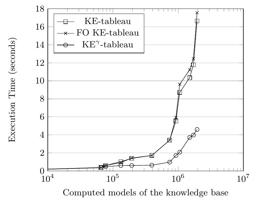
Refer to caption
Figure 3: Comparison among the KE-system, FO KE-system, and KEγ-system.

The benchmarking process is based on a huge amount of KBs of different size and kind, constructed ad-hoc for the purpose of comparing the three mentioned systems, and on some real-world ontologies developed by the authors.

5 Conclusions and future work

We presented an improvement, called KEγ-tableau, of the KE-tableau in [3] for the most widespread reasoning tasks for \mathcal​D​L𝐃4,×\mathcal{DL}_{\mathbf{D}}^{4,\!\times}-TBoxes and \mathcal​D​L𝐃4,×\mathcal{DL}_{\mathbf{D}}^{4,\!\times}–ABoxes. These reasoning problems are addressed by translating \mathcal​D​L𝐃4,×\mathcal{DL}_{\mathbf{D}}^{4,\!\times}-KBs and queries in terms of formulae of the set-theoretic language 𝟦​𝖫​𝖰​𝖲\mathcal​D​LD4,​×R\mathsf{4LQS}_{\scriptscriptstyle{\mathcal{DL}_{\lx@scalerel@obj{\mathbf{D}}}^{\lx@scalerel@obj{4,\!\times}}}}^{R}. The procedure introduced in this paper generalizes the KE-elimination rule in such way as to incorporate the γ\gamma-rule, that is the expansion rule handling universally quantified formulae. The KEγ-tableau procedure has remarkable aftermath, since its implementation is markedly more efficient in terms of space and execution time than the KE-system [5] and the implementation (FO KE-system) of the FO KE-tableau[11], as observed in our experimental tests.

We plan to modify the set-theoretic fragment underpinning the reasoner so as to include a restricted version of the operator of relational composition in order to be able to reason with DLs admitting full existential and universal quantification. Results and notions presented in [10] will be of inspiration for such a task. We also intend to improve our reasoner so as to deal with the reasoning problem of ontology classification. We shall compare the resulting reasoner with existing well-known reasoners such as Hermit [7] and Pellet [14], providing also some benchmarking. In addition, we plan to allow data type reasoning by either integrating existing solvers for the Satisfiability Modulo Theories (SMT) problem or by designing ad hoc new solvers. Finally, as each branch of a KEγ-tableau can be independently computed by a single processing unit, we plan to implement a parallel version of the software by using the Nvidia CUDA framework.

References

  • [1] D. Cantone and M. Nicolosi-Asmundo. On the satisfiability problem for a 4-level quantified syllogistic and some applications to modal logic. Fundamenta Informaticae, 124(4):427–448, 2013.
  • [2] D. Cantone, M. Nicolosi-Asmundo, and D. F. Santamaria. Conjunctive Query Answering via a Fragment of Set Theory. In Proc. of ICTCS 2016, Lecce, September 7-9, CEUR-WS Vol. 1720, pp. 23–35, 2016.
  • [3] D. Cantone, M. Nicolosi-Asmundo, and D. F. Santamaria. A set-theoretic approach to ABox reasoning services. In Van Woensel W. Kontchakov R. Sadri F. Roman D. Costantini S., Franconi E., editor, Rules and Reasoning. RuleML+RR 2017, volume 10364 of Lecture Notes in Computer Science, pages 87–102. Springer, 2017.
  • [4] D. Cantone, M. Nicolosi-Asmundo, and D. F. Santamaria. A set-theoretic approach to ABox reasoning services. CoRR, 1702.03096, 2017. Extended version.
  • [5] D. Cantone, M. Nicolosi-Asmundo, and D. F. Santamaria. A C++ reasoner for the description logic \mathcal​D​L𝐃4,×\mathcal{DL}_{\mathbf{D}}^{4,\!\times}. In Proceedings of CILC 2017, 26-29 September 2017, Naples, Italy. CEUR WS, ISSN 1613-0073, Vol. 1949, pp. 276-280., 2017.
  • [6] M. D’Agostino. Tableau methods for classical propositional logic. In Marcello D’Agostino, Dov M. Gabbay, Reiner Hähnle, and Joachim Posegga, editors, Handbook of Tableau Methods, pages 45–123. Springer, 1999.
  • [7] B. Glimm, I. Horrocks, B. Motik, G. Stoilos, and Z. Wang. HermiT: An OWL 2 Reasoner. Journal of Automated Reasoning, 53(3):245–269, 2014.
  • [8] I. Horrocks, O. Kutz, and U. Sattler. The even more irresistible SROIQ. In Proc. 10th Int. Conf. on Princ. of Knowledge Representation and Reasoning, (Doherty, P. and Mylopoulos, J. and Welty, C. A., eds.), pages 57–67. AAAI Press, 2006.
  • [9] M. Krötzsch. OWL 2 Profiles: An Introduction to Lightweight Ontology Languages, pages 112–183. Springer Berlin Heidelberg, Berlin, Heidelberg, 2012.
  • [10] Cristiá M. and G. Rossi. A decision procedure for restricted intensional sets. In Automated Deduction - CADE 26 - 26th Int. Conf. on Automated Deduction, Gothenburg, Sweden, August 6-11, 2017, Proceedings, pages 185–201, 2017.
  • [11] M.Mondadori M. D’Agostino. The taming of the cut. classical refutations with analytic cut. Journal of Logic and Computation, 4:285–319, 1994.
  • [12] B. Motik and I. Horrocks. OWL datatypes: Design and implementation. In Proc. of the 7th Int. Semantic Web Conference (ISWC 2008), volume 5318 of LNCS, pages 307–322. Springer, October 26–30 2008.
  • [13] M. Ortiz, R. Sebastian, and M. Šimkus. Query answering in the Horn fragments of the description logics \mathcal​S​H​O​I​Q\mathcal{SHOIQ} and \mathcal​S​R​O​I​Q\mathcal{SROIQ}. In Proc. of the 22th Int. Joint Conf. on Artificial Intell. - Vol.Two, IJCAI’11, pages 1039–1044. AAAI Press, 2011.
  • [14] E. Sirin, B. Parsia, B. C. Grau, A. Kalyanpur, and Y. Katz. Pellet: A practical OWL-DL reasoner. Journal of Web Semantic, 5(2):51–53, 2007.
  • [15] R. M. Smullyan. First-order Logic. Dover books on advanced Math. Dover, 1995.