The second boundaries of Stability Zones and the angular diagrams of conductivity for metals having complicated Fermi surfaces.
Abstract
We consider some general aspects of dependence of magneto-conductivity on a magnetic field in metals having complicated Fermi surfaces. As it is well known, a nontrivial behavior of conductivity in metals in strong magnetic fields is connected usually with appearance of non-closed quasiclassical electron trajectories on the Fermi surface in a magnetic field. The structure of the electron trajectories depends strongly on the direction of the magnetic field and usually the greatest interest is caused by open trajectories that are stable to small rotations of the direction of . The geometry of the corresponding Stability Zones on the angular diagram in the space of directions of represents a very important characteristic of the electron spectrum in a metal linking the parameters of the spectrum to the experimental data. Here we will consider some very general features inherent in the angular diagrams of metals with Fermi surfaces of the most arbitrary form. In particular, we will show here that any Stability Zone actually has a second boundary, restricting a larger region with a certain behavior of conductivity. Besides that, we shall discuss here general questions of complexity of the angular diagrams for the conductivity and propose a theoretical scheme for dividing the angular diagrams into “simple” and “complex” diagrams. The proposed scheme will in fact also be closely related to behavior of the Hall conductivity in a metal in strong magnetic fields. In conclusion, we will also discuss the relationship of the questions under consideration to the general features of an (abstract) angular diagram describing the behavior of quasiclassical electron trajectories at all energy levels in the conduction band.
I Introduction.
We will consider here phenomena connected with some special properties of the quasiclassical electron motion along the Fermi surface in normal metals. According to standard approach, we will describe the electron states in a metal with the aid of the number of the energy band and the value of the quasimomentum . As it is well known, any value of should in fact be considered as an infinite set of “equivalent” values , differing by vectors of the reciprocal lattice . The basis of the reciprocal lattice can be given by the vectors
where represent a basis of the direct lattice of a metal. The energy of an electron state in the band is given by a three-periodic function in the - space, which can also be considered as a function on the three-dimensional torus , given by the factorization of the - space with respect to the reciprocal lattice vectors
As it is also well known, the electron states in normal metals are occupied, if their energy is less than the Fermi energy , and are empty if . So, we have in any normal metal a finite number of completely filled energy bands, a finite number of partially filled energy bands (conduction bands) and an infinite number of empty energy bands. The Fermi surface of a normal metal is defined as the union of the surfaces in the - space, where the index numerates all the conduction bands. In all our considerations here we will assume that the Fermi surface represents a smooth 3-periodic non-selfintersecting surface in the - space, which can contain different connected components.
More precisely, a collective electron state in a metal can be described in the kinetic approximation by a one-particle distribution function , which can be different from or just in a narrow region near the Fermi surface. So, all the kinetic properties of a normal metal are defined in fact by electron states near the surface .
The quasiclassical evolution of electron states in the presence of external electric and magnetic fields can be described with the aid of the adiabatic system
which can be considered as a dynamical system on the torus .
The function satisfies the one-particle kinetic equation
where represents the collision integral.
In our considerations here we will consider the electric field as infinitely small. At the same time, the value of the magnetic field is supposed to be large enough. More precisely, we will assume here the condition , where plays the role of the mean free electron motion time and has the meaning of the cyclotron frequency of the electron motion in crystal. As a corollary, the phenomena considered here will be actually connected with the geometry of trajectories of the system
| (I.1) |
System (I.1) conserves the energy of an electron state and also the projection of the quasimomentum on the directions of . So, the trajectories of system (I.1) in the - space can be obtained as the intersections of the constant energy levels with the planes orthogonal to . Let us say, however, that in spite of this analytical integrability of system (I.1) the geometry of its trajectories in - space can in fact be rather complicated for the energy levels having complicated form (Fig. 1). It is easy to see also that in kinetic phenomena in normal metals only the trajectories lying on the Fermi surface can play an essential role.

An important role of the geometry of trajectories of system (I.1) for the magneto-transport phenomena in metals was first revealed by the school of I.M. Lifshitz (I.M. Lifshitz, M.Ya. Azbel, M.I. Kaganov, V.G. Peschansky) in 1950’s. In particular, a crucial difference between the closed and open trajectories of system (I.1), which is manifested in the behavior of the magneto-conductivity in strong magnetic fields, was first described in detail in the papers [1, 2, 3]. Thus, it was first pointed out in the paper [1] that the closed and the open periodic trajectories of system (I.1) give quite different contributions to the magneto-conductivity in the plane, orthogonal to , in the limit . More precisely, the contribution of the closed trajectories in the plane, orthogonal to , is almost isotropic in the limit and decreases rapidly when . The general conductivity tensor in the presence of only closed trajectories on the Fermi level can be expressed by the following asymptotic formula
| (I.2) |
where , and is analogous to the same formula for the free electron gas.
At the same time, the contribution of the open periodic trajectories to the conductivity is strongly anisotropic in the plane orthogonal to and decreases just in one direction (coinciding with the mean direction of the open trajectories in - space) in the limit . The general formula for the asymptotic behavior of the conductivity tensor can be written in this case in the form
| (I.3) |
where the direction of the - axis coincides with the mean direction of the open trajectories in the - space (here and everywhere the notation means just some constant of the order of ).
The open trajectories of system (I.1), considered in [2, 3], have more general form and are not periodic in the - space. However, all the (quasiperiodic) trajectories, considered in [2, 3], have a mean direction in the - space and also give anisotropic contribution to the conductivity in strong magnetic fields. Generally speaking, the asymptotic behavior of conductivity tensor can not be described here by a simple formula (I.3), however, it also shows vanishing of the conductivity just along one direction in the plane, orthogonal to , and a finite conductivity in the orthogonal direction in the limit . Many aspects, connected with the geometry of trajectories of system (I.1), were described in the papers [4, 5, 6, 7, 8]. Certainly, the references given here do not give a complete list of papers, which could be mentioned in connection with this rather wide area.
The general problem of classification of open trajectories of system (I.1) was set by S.P. Novikov ([9]) and was intensively studied in his topological school (S.P. Novikov, A.V. Zorich, S.P. Tsarev, I.A. Dynnikov). Due to rather deep mathematical results (see [10, 11, 12, 13, 14]), obtained in the study of this problem from the topological point of view, the problem of description of possible types of open trajectories of system (I.1) is now solved, so we can use in fact the full classification of trajectories of system (I.1) in our study of transport phenomena in normal metals.
The most important role in the classification of open trajectories of system (I.1) is played in fact by a description of the stable open trajectories of (I.1), i.e. the open trajectories which do not change essentially their global geometry under small rotations of or variations of the energy level . As follows from the results of [10, 11, 13], the stable open trajectories of system (I.1) possess the following remarkable properties:
1) Every stable open trajectory of system (I.1) in - space lies in a straight line of a finite width in the plane orthogonal to and passes through it from to (Fig. 2);
2) The mean direction of all stable open trajectories in - space is given by the intersection of the plane orthogonal to with some locally stable integral plane in the - space.
Let us note here also that the property (1) was in fact first formulated by S.P. Novikov in [9] in the form of a conjecture and was later proved in the papers [10, 11, 13] for the open trajectories having stability properties in the sense pointed above.

The remarkable properties of the stable open trajectories of system (I.1) can be observed in direct measurements of magneto-conductivity of normal metals in strong magnetic fields. Thus, due to the geometric properties of the stable open trajectories, their contribution to the conductivity in the plane orthogonal to is strongly anisotropic in the limit , such that the direction of the lowest conductivity (in - space) coincides with the mean direction of the trajectories in - space. Due to the stability of these trajectories with respect to small rotations of , this situation takes place also for all close directions of , which allows to observe also the integral plane , defined by the property (2), in the case of the presence of stable open trajectories on the Fermi surface. Let us note here that a plane is called integral in the - space, if it is generated by two reciprocal lattice vectors , :
In the - space the same plane can be represented by an indivisible triple of integer numbers with the aid of the equation
where represent the basis of the direct lattice.
The numbers were introduced in [15] as topological characteristics of electron spectra in metals, which can be observed in the transport phenomena in strong magnetic fields. According to [15], these numbers can be called topological quantum numbers observable in the conductivity of normal metals. In accordance to the picture represented above, we can in general distinguish special “Stability Zones” in the space of directions of (the unit sphere ), corresponding to the presence of stable open trajectories on the Fermi surface, which can be observed in the study of magneto-conductivity in strong magnetic fields.
Just by definition, we will call the Stability Zone a complete region in the space of directions of , where we have stable open trajectories of system (I.1) on the Fermi surface, corresponding to the same topological quantum numbers . The Stability Zones, defined in this way, can be also called exact mathematical Stability Zones and represent some regions with piecewise smooth boundaries on the unit sphere (Fig. 3). It is not difficult to see that any Stability Zone is invariant under the transformation and in most cases consists of two opposite regions on the unit sphere.
Let us say here, that the geometry of the Stability Zones and the values of represent rather nontrivial characteristics of the electron spectra in metals, which are not defined just by the topology of the Fermi surface and depend also on its geometrical parameters in rather nontrivial way. Let us note also that the full sets of exact mathematical Stability Zones and the topological numbers can be rather nontrivial for a metal having complicated Fermi surface. We would like to give here a reference to the paper [16], containing a description of many mathematical results related to the behavior of trajectories of system (I.1) with an arbitrary dispersion relation and the geometry of the corresponding Stability Zones in the space of directions of . We would also like to specially mention here the paper [17] that presents a rather convenient method for investigating the geometry of the Stability Zones for specific dispersion relations and also containing applications of this method to important analytical examples. Let us also say that a large number of physical consequences arising from the results of mathematical study of the system (I.1) were presented in the papers [18, 19, 20, 21].

The numbers describe the “geometric properties” of the tensor for and represent well observed experimental quantities in the limit . At the same time, the analytic dependence of the tensor both on the value and the direction of for can be in fact rather nontrivial even under the implementation of the condition ([22]). The reason for such behavior of the conductivity is actually the appearance of periodic open trajectories of system (I.1) for special directions , which introduce irregularity in the limiting values of when . As a result, the angular dependence of the tensor is actually rather irregular for even for big enough values of the parameter . Let us say, that the appearance of periodic open trajectories of system (I.1) for irrational directions of represents in general a nontrivial fact, closely connected with arising of a special integral plane for every Stability Zone. Thus, the periodic open trajectories of system (I.1) arise on the Fermi surface at whenever the intersection of the plane orthogonal to and the plane has a rational direction. Its not difficult to see, that the corresponding directions of form in general an everywhere dense set in the Zone .
Another important feature of the periodic open trajectories of system (I.1), following from the topological structure of the system (I.1) for , is that they actually exist also on some special sets outside the Stability Zone near its boundary (let us note also here that this phenomenon can appear also for some special examples of simple Fermi surfaces, see e.g. [23]). The corresponding directions of are not included in the Stability Zones since the periodic trajectories are no longer stable outside the Zones . In general, we can have either periodic open trajectories or very long closed trajectories on the Fermi surface for directions of , close to the boundary of a Stability Zone . As a result, the exact boundary of a Stability Zone is usually unobservable in direct conductivity measurements even under the condition . As was pointed out in [22], we have to introduce actually extended “experimentally observable” Stability Zones on the angular diagram, which arise as observable Stability Zones in the direct measurements of conductivity (Fig. 4).

At the same time, the exact boundary of a Stability Zone represents an important characteristic of the electron spectrum in metal being closely connected with the geometric parameters of the Fermi surface. As was pointed out in [24], the boundary of an exact mathematical Stability Zone can be actually determined in the study of oscillation phenomena in metals like the cyclotron resonance phenomenon or different types of quantum oscillations. As was shown in [24], the picture of (classical or quantum) oscillations undergoes sharp changes at the boundary of exact mathematical Stability Zone, which can be clearly registered in the dependence of the oscillations on the value of . More precisely, the change in the dependence of the oscillating values on the value of is given by abrupt disappearance of one of the main oscillating terms (one oscillating harmonic) after crossing the boundary of on the angular diagram.
In the present paper we will consider some general aspects of the angular diagram of conductivity and the structure of the Stability Zones on for metals having (arbitrary) complicated Fermi surfaces. In particular, we are going to show here that the Stability Zones have in fact “the second boundaries” on the angular diagram in the space of directions of , which can be also detected in the same study of oscillation phenomena in strong magnetic fields. The region , restricted by the second boundary of a Stability Zone , always contains the Zone and can have different sizes depending on the geometry of the Fermi surface. Thus, we can have both the situations when the second boundary is close to the (first) boundary of a Stability Zone or it is located rather far from the boundary of . In particular, the region can contain either the whole “experimentally observable Stability Zone” in a given experimental study of conductivity or just a part of the Zone .
One of the essential properties of the domain between the first and the second boundary of a Stability Zone is that it can not contain directions of corresponding to the presence of any stable open trajectories on the Fermi surface (at the same time, the unstable periodic trajectories can arise here for special directions of mentioned above). In the present paper we consider different phenomena arising in the domain at different directions of magnetic field. As will be shown, the picture of (classical and quantum) oscillation phenomena has in this domain rather specific features which can in fact be used for the investigation of the geometry of the Fermi surface. At the same time, the direct conductivity measurements (at ) also have here special features which will be discussed in the next sections. We will also consider here the most general features of the location of the Stability Zones and the corresponding additional areas on the angular diagram.
Another aspect which we will touch in the present paper is the distribution of the Stability Zones on a general angular diagram. As we will show, it is natural to divide actually all the angular diagrams into “simpler” (Type A) and “more complicated” (Type B) diagrams in the general case. Both Types (A and B) represent completely general classes that cover the whole set of angular diagrams and are equally possible from theoretical point of view. At the same time, it seems that for most of the real materials we should actually expect the appearance of Type A diagrams with a much higher probability than diagrams of the Type B. In most cases Type A angular diagrams are characterized by the presence of only a finite number of Stability Zones on while the angular diagrams of Type B generically contain an infinite number of different Stability Zones on the unit sphere. Another important feature of the angular diagrams of Type B is that we should also expect here special directions of corresponding to appearance of more complicated (chaotic) open trajectories on the Fermi surface, which leads to the appearance of very special asymptotic regimes of conductivity behavior in strong magnetic fields. As a consequence, the appearance of a Type B angular diagram gives a much greater variety of different types of conductivity behavior, observed experimentally. As we will also show here, the angular diagrams of different types can be conveniently distinguished by a study of the Hall conductivity outside the Stability Zones at .
In sections II and III we will represent a detailed consideration of the structure of system (I.1) for and consider phenomena connected with special features of its trajectories in this domain. Our considerations here will be based on topological results, obtained in recent topological investigations of the S.P. Novikov problem ([10, 11, 13, 14, 16]) and describing the topology of “carriers of open trajectories” in the case of the presence of stable open trajectories on the Fermi surface. As we will see, the topological description of the structure of system (I.1) in the Stability Zones gives in fact also a good possibility to describe the properties of its trajectories in the domain . As we have said already, the main considerations will be connected with the oscillation phenomena in this domain, having classical or quantum nature.
In section IV we discuss different Types of the angular diagrams and their connection with types of the boundaries of Stability Zones and the Hall conductivity behavior outside the Stability Zones.
In section V we discuss a connection between the angular diagrams for conductivity of metals and the angular diagrams for a full dispersion relation , which describe the behavior of trajectories of system (I.1) at all energy levels . Let us note here that although the introduction of an angular diagram for the full dispersion relation has a somewhat abstract character in the theory of normal metals, such a comparison is, as it seems to us, quite useful from a methodological point of view.
II The structure of the Fermi surface and the geometry of trajectories of system (I.1) for .
Let us start with the description of the structure of the Fermi surface for , which will also give a description of its structure in the domain . As follows from rather deep topological theorems proved in [10, 11, 13, 14, 16], in the presence of stable open trajectories on the level the structure of the corresponding connected component of the Fermi surface can be described in the following way:
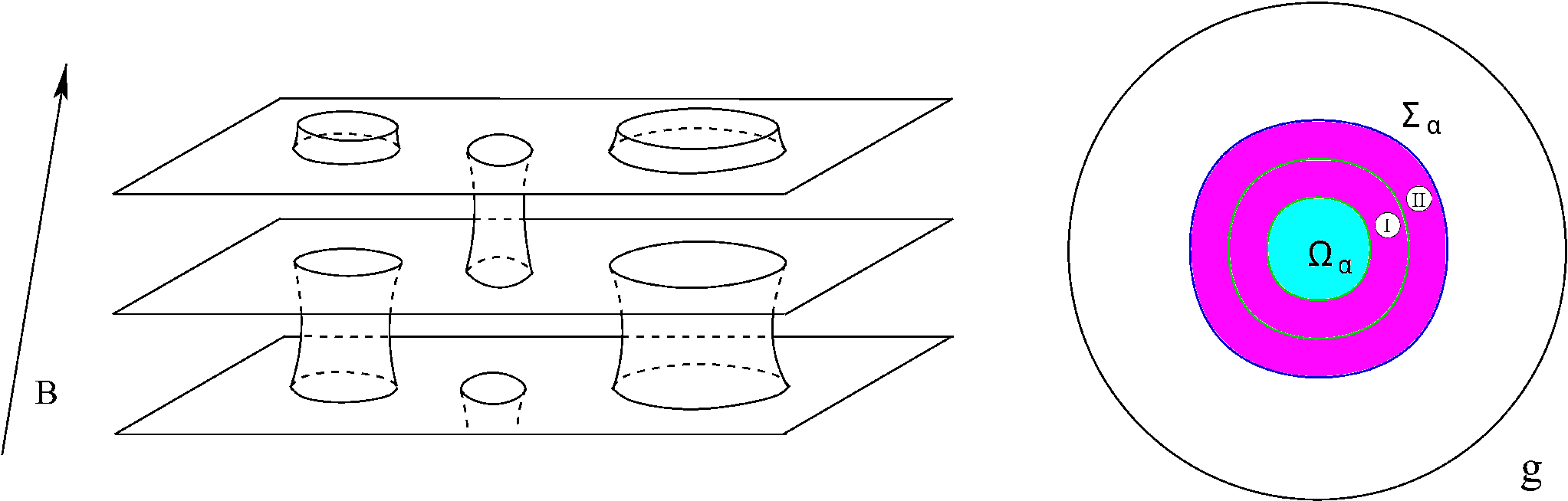
Let us imagine a set of parallel integral planes in the - space, connected by cylinders of finite heights (Fig. 5).

It is not difficult to see, that if we choose the direction of close to the directions of the axes of the cylinders we will have a cylinder of closed trajectories on every cylinder, shown at Fig. 5, restricted by singular closed trajectories on the Fermi surface (Fig. 6). Let us note, that we admit here also the appearance of cylinders of closed trajectories having a point as a base. The cylinders of the last type can be called trivial from the topological point of view. Theoretically, it is also possible to admit a compound structure of cylinders connecting planes. This, however, does not affect further conclusions and is extremely unlikely for real Fermi surfaces, so we will not consider this complication here.

We can see then, that the integral planes at Fig. 6 are actually separated from each other by the cylinders of closed trajectories and represent “carriers of open trajectories” of system (I.1) on the Fermi surface. Thus, every carrier of open trajectories represents a periodically deformed integral plane (with holes) in the - space, which is locally stable under small rotations of (Fig. 7). It is easy to see here, that every open trajectory at Fig. 6 has a mean direction in the - space, given by the intersection of the plane, orthogonal to , and the integral plane, corresponding to the carriers of open trajectories.

Let us say here, that Fig. 5 and 6 represent just a topological structure of the Fermi surface carrying stable open trajectories and can be visually much more complicated. The representation of the Fermi surface shown at Fig. 5, 6 is not uniquely defined, thus, we get different representations (of the same Fermi surface) in the form Fig. 5, 6 for directions of lying in two different Stability Zones , . At the same time, the existence of the structure, shown at Fig. 5, 6, on any Fermi surface carrying stable open trajectories of system (I.1) represents a rigorous topological theorem, valid in the most general case (see [10, 11, 13, 14, 16]).
It is easy to see that the integral planes at Fig. 6 can be actually divided into two types according to the direction of the electron motion (back or forward) on the corresponding open trajectories. In the same way, all the cylinders of closed trajectories can be divided into two different types according to the type of the closed trajectories (electron type or hole type) on them. We will assume here that we have just two nonequivalent integral planes (having different types) in the representation of the Fermi surface according to Fig. 5, 6. As can be shown, the Fermi surfaces, having bigger number of nonequivalent integral planes in the - space in their representation above, should have in fact very high genus, so this situation should be actually quite rare for real metals. At the same time, we will assume here that we have at least two or more nonequivalent cylinders of closed trajectories in the representation of the Fermi surface according to Fig. 5, 6 (where the number of topologically nontrivial cylinders is actually equal to ).
The exact boundary of a Stability Zone is defined by disappearance of one of the cylinders from the set of nonequivalent nontrivial cylinders of closed trajectories on the Fermi surface. Thus, for directions of , close to the boundary of a Stability Zone, the height of the corresponding cylinder of closed trajectories become very small and vanishes at the boundary of . After crossing the boundary of the corresponding cylinder does not separate a pair of integral planes anymore, so the trajectories can now jump from one plane to another (Fig. 8).

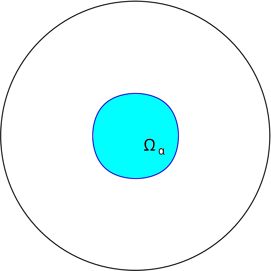
Let us note here, that in general we can have both the situation when the whole boundary of a Stability Zone is defined by disappearance of the same cylinder of closed trajectories and the situation when different parts of the boundary of correspond to disappearance of different cylinders from the set. Let us say here that in the first case the Stability Zone has a simple boundary (Fig. 9) and in the second case the Stability Zone has a compound boundary (Fig. 10). In general, our considerations here will be applicable to both of the above cases.
 |
 |
 |
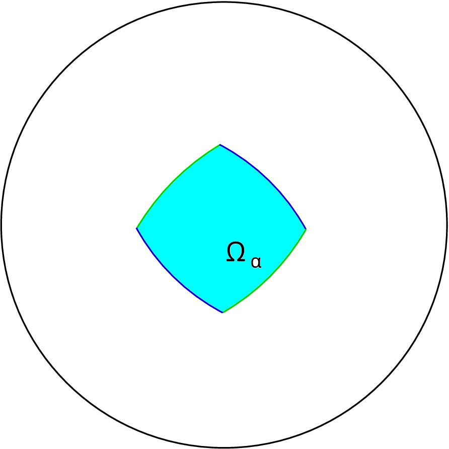 |
As we said already, after the disappearance of one of the cylinders of closed trajectories at Fig. 6 the integral planes are not separated from each other anymore and the trajectories of system (I.1) can now jump from one plane to another. At the same time, the geometry of trajectories of (I.1) still can be easily described in the vicinity of the boundary of the Zone . Indeed, in the immediate vicinity of the boundary of the Fermi surface shown at Fig. 6 is still divided into pairs of connected integral planes, which are separated from each other by the remaining cylinders of closed trajectories of system (I.1). This situation takes place until the second cylinder of closed trajectories on the Fermi surface disappears, so that jumps of the trajectories of system (I.1) between connected pairs of former carriers of open trajectories become possible. Let us call the corresponding curve in the space of directions of the second boundary of a Stability Zone and denote by the region, restricted by this curve on the angular diagram. Let us note here, that the second boundary of a Stability Zone can be also simple or compound (Fig. 11) depending on the geometry of the Fermi surface. In general, the form of the second boundary of a Stability Zone is not closely connected with the form of its first boundary, as can be seen from the examples shown at Fig. 12.
 |
 |
![[Uncaptioned image]](1804.10762v4/Example1.png)
![[Uncaptioned image]](1804.10762v4/Example2.png)
![[Uncaptioned image]](1804.10762v4/Example3.png)
![[Uncaptioned image]](1804.10762v4/Example4.png)
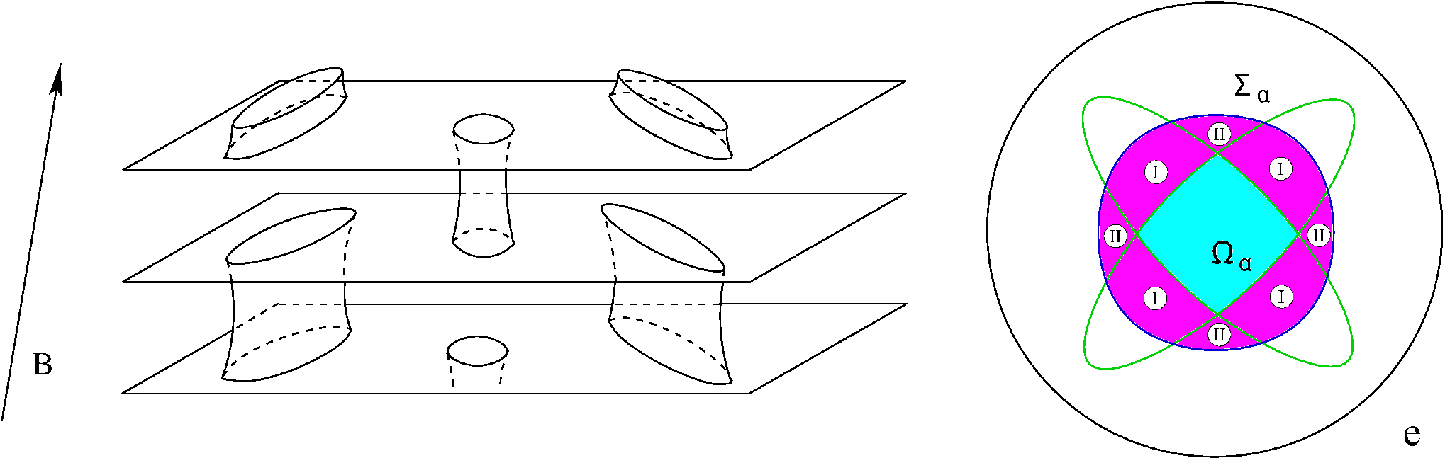
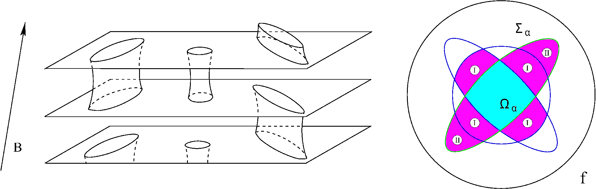
Just by definition, the domain is defined as the domain, adjacent to , where the Fermi surface can be represented as a set of pairs of connected integral planes with Topological Numbers , which are separated by cylinders of closed trajectories of system (I.1). As can be seen, the domain can be connected (Fig. 12, a, c, e, g) or can consist of several connected components (Fig. 12, b, d, f). The boundary of every connected component of the domain can be divided into two parts, i.e. the internal boundary (adjacent to ) and the external boundary. What is important here is that for every connected component of its internal and external boundaries correspond to disappearance of cylinders of closed trajectories of opposite types (electron type or hole type) (Fig. 12). It can be seen also that we can have both the situations when the connected pairs of former carriers of open trajectories are defined uniquely for the whole domain (Fig. 12, a, c, e, g), or represented in different ways in different parts of (Fig. 12, b, d, f). One more feature which can be noted here is that even for a given set of connected pairs of the former carriers of open trajectories we can have parts of where they are connected through one former cylinder of closed trajectories or where they are connected through two (or more) former cylinders of closed trajectories (parts I and II at Fig. 12, e, f, g). The corresponding regions are also separated by lines where we have disappearance or appearance of a cylinder of (short) closed trajectories, which can be also observed in the study of oscillation phenomena in the corresponding frequency range.
The domain
can be called the “derivative” of the Stability Zone since the Fermi surface keeps here a part of its special representation in the Zone , which still gives an effective description of trajectories of system (I.1) in this domain.
To describe the trajectories of system (I.1) on the connected pairs of the former carriers of open trajectories we have to note first that the trajectories that have jumps on a fixed cylinder connecting a pair of integral planes (Fig. 8) form narrow strips restricted by two singular trajectories with close values of . The value of is constant at every trajectory of system (I.1), so all these strips are represented just by straight narrow strips after the projection on a plane, containing the vector . Using the projection on the plane, containing the vector , we can mark the corresponding cylinders just by circles (or segments) of the corresponding size (), which form a periodic structure in the plane (Fig. 13). Every trajectory of system (I.1) will be represented now by a straight line , which can have endpoints at the circles, introduced above. The singular trajectories of system (I.1) are represented by lines, tangential to the circles, and separate trajectories of substantially different geometry on the Fermi surface. It is not difficult to see that for generic directions of , such that the intersection of the plane orthogonal to and the plane has an irrational direction in - space, every trajectory of system (I.1) will be actually represented by a line of a finite size, restricted by two circles at both ends. As a result, the pair of the former carriers of open trajectories will be divided itself into cylinders of closed trajectories of system (I.1), which will have rather big sizes if is close to the boundary of the Zone .

Let us consider here the simplest situation when the jumps of the trajectories between two former carriers of open trajectories occur just on one cylinder from the set of the former cylinders of closed trajectories, connecting these carriers. Fig. 13 represents schematic division of a connected pair of the former carriers of open trajectories into layers of long closed trajectories after crossing the boundary of the Zone . Every colored strip at Fig. 13 represents the projection of trajectories of approximately the same form on a plane () containing the vector . As can be easily seen, we will have here exactly three nonequivalent layers of significantly different long closed trajectories, separated by singular closed trajectories, on every connected pair of former carriers of open trajectories in the - space (Fig. 14).

At the same time, if the intersection of the plane, orthogonal to , and the plane has a rational direction in the - space and the value of is small enough we can still have periodic open trajectories on the former carriers of open trajectories after crossing the boundary of the Zone (Fig. 15). As can be easily seen, we will have in this case just one layer of long closed trajectories and two (opposite) layers of periodic open trajectories on a connected pair of former carriers of open trajectories. It is easy to see also, that in the picture described above we can not have open trajectories of system (I.1) which could be stable with respect to all small rotations of the direction of .

Easy to see that the long closed trajectories arising near the boundary of the Stability Zone have a specific form shown at Fig. 16. We can see, that we should have here three different “sets” of the long closed trajectories according to the number of nonequivalent layers of significantly different closed trajectories on the Fermi surface. We can see also, that we can write the approximate equality
for the areas, restricted by the trajectories, shown at Fig. 16, in the plane, orthogonal to in the - space.
In the same way, we can write also
for the periods of motion along the trajectories shown at Fig. 16, or
for the corresponding cyclotron frequencies.

More precisely, the layers of long closed trajectories, shown at Fig. 14, should contain also additional singularities, arising at the bases of cylinders of short closed trajectories, separating the pairs of the former carriers of open trajectories (Fig. 17). These singularities always appear at the boundaries of singular two-dimensional discs, orthogonal to , which are actually invisible at the projection on the plane . This means actually that the number of topologically nonequivalent cylinders of long closed trajectories (separated by singular trajectories) is in fact greater than 3. However, if the length of the closed trajectories is very big, we can still introduce three sets of similar long closed trajectories corresponding to three essentially different periods , , as it is shown at Fig. 17. We can note also that when the long closed trajectories become shorter we should have a “splitting” of the periods , , into a bigger set , corresponding to the number of extremal trajectories on all topologically different cylinders of closed trajectories described above.

It can be shown also, that in the case when the number of nonequivalent cylinders connecting former carriers of open trajectories is equal to 2, we can introduce five periods , , , , (the number of the cylinders of long closed trajectories is actually greater), which can be numerated in such a way, that we can write the relations
| (II.1) |
or
| (II.2) |
As we said already, this situation can arise in special regions in the domain (regions II at Fig. 12, e, f, g), which are separated by special curves, observable in the study of oscillation phenomena at high frequencies (). We should note also, that the relations (II.1) and (II.2) can be written only for long enough closed trajectories and we should also observe here a splitting of the periods , , , , into a bigger set when the trajectories become shorter. Theoretically we can consider also even more complicated cases, where the number of typical periods is even greater, however, they are very unlikely for real metals. In particular, we will always have the situation with three periods , , in the vicinity of “regular” points of the first boundary of a Stability Zone (regions I at Fig. 12, e, f, g).
III The geometry of the long closed trajectories and the behavior of conductivity in the domain .
What can we say about the behavior of the magneto-conductivity or, more generally, the effects connected with the presence of a strong magnetic field in the case when the direction of belongs to the domain ? Let us say first of all that the domain always contains a narrow region near the boundary of the Zone where the length of the long closed trajectories is very large. As a corollary, the condition in this region is obviously violated and the long closed trajectories are indistinguishable here from the open trajectories from the experimental point of view. The conductivity tensor (for available values of ) has here the same geometric properties as in the Stability Zone and the same is also valid for its analytic properties (see [22]). As we have said already, the position of the boundary of can be detected in general by the study of special features of the cyclotron resonance phenomenon (at high external frequencies) or other (quantum) oscillation phenomena (see [24]), which are connected with the disappearance of a cylinder of (short) closed trajectories on the Fermi surface.
As we have also said already, the position of the second boundary of a Stability Zone is to some extent independent of the position of the first boundary. In particular, we can have the situation when the second boundary of a Stability Zone is very close to its first boundary, such that the domain represents a narrow region in the vicinity of the boundary of . In this case the period of the electron motion over the long closed trajectories can be very big and the condition will be in fact violated everywhere in (Fig. 18). In this case we can just observe the first and the second boundaries of a Stability Zone with the aid of study of the oscillation phenomena inside the “experimentally observable” Stability Zone .

Let us note here that in the standard setting of the experimental study of the cyclotron resonance phenomenon it is often convenient to choose the direction of the electric field in the incident wave orthogonal to the direction of the constant magnetic field . In this case the endpoints on the “trivial” cylinders of closed trajectories (Fig. 6) give no contribution to the picture of oscillations, so, only the extremal trajectories on the topologically nontrivial cylinders of closed trajectories bring oscillating terms in the dependence of physical quantities on the value of (or ). If we assume also that every topologically nontrivial cylinder of closed trajectories contains just one extremal trajectory then the number of the oscillating terms in a Stability Zone should be exactly , where is the genus of the Fermi surface.
As was pointed out in [24], the picture of oscillations should undergo a rapid transformation on the boundary of any Stability Zone due to the disappearance of a cylinder of closed trajectories after crossing the boundary of on the angular diagram. Thus, for a Fermi surface of genus 3 we should observe a rapid transformation of a picture, containing 2 oscillating terms, to a picture, containing just one oscillating term, at the first boundary of a Stability Zone. If we assume now that the second boundary is very close to the first boundary of a Stability Zone and the long closed trajectories do not give any contribution to the oscillation phenomena inside the domain , we expect then a rapid transformation of the picture, containing just one oscillating term, to a picture, containing no oscillating terms, at the second boundary of a Stability Zone (Fig. 19). For Fermi surfaces having higher genera the picture of oscillations should be more complicated. For comparison, for a Fermi surface of genus 4 we should observe a rapid transformation of a picture, containing 3 oscillating terms, to a picture, containing 2 oscillating terms, at the first boundary of a Stability Zone and a rapid transformation of the picture, containing 2 oscillating terms, to a picture, containing just one oscillating term, at the second boundary (Fig. 20). Let us note also that the pictures represented at Fig. 19 and Fig. 20 can be somewhat schematic in nature since the form of the oscillation peaks in the oscillating terms can be different in different situations.


Another special feature, which can arise on complicated Fermi surfaces is the disappearance of additional cylinders of closed trajectories between the first and the second boundaries of a Stability Zone (Fig. 12, e, f, g). In this case the full picture of transformations of the cyclotron oscillations caused by the rotation of can resemble the situation shown at Fig. 21.

As we said already, in the case of a narrow domain , lying entirely in the experimentally observable Stability Zone , rapid transformations of the oscillation picture, similar to those shown at Fig. 19, 20, 21, give the only evidence of the existence of the first and the second boundaries of a Stability Zone .
We can consider now the “intermediate situation” when the long closed trajectories in the domain can have “intermediate” length, such that we have the relations
| (III.1) |
where is the period of the electron motion over the long closed trajectory. This means that the domain has only a partial intersection with the “experimentally observable” Stability Zone (Fig. 22) and we can observe some special features in the conductivity behavior in the domain .

It is easy to see that we should observe here a special picture of oscillation phenomena (classical or quantum) connected with the long closed trajectories arising in . Let us specially discuss here the picture of the cyclotron resonance oscillations connected with the closed trajectories satisfying condition (III.1).
In the standard setting of experimental investigation of the cyclotron resonance phenomenon we assume that the magnetic field is parallel to the surface of a metal sample and we explore the behavior of the surface current in the field of an incident electromagnetic wave. The interaction of electrons with the wave field occurs in a narrow skin layer which is usually much less than the size of the cyclotron orbit in the - space. In generic case the long closed trajectories are inclined with respect to the surface of a sample in the - space, so we have the picture of electron motion through the skin layer schematically represented at Fig. 23. We can see, that in the - space the electron trajectory has in general also a drift along the direction of . Let us note here that for the long closed trajectories this drift is actually rather small since the average of the value is close to zero on the trajectories of this type. (Strictly speaking, this property can be in fact violated for very complicated Fermi surfaces of very high genera).

According to standard theory of the cyclotron resonance (see e.g. [25, 26, 7, 27, 28]), every extremal closed trajectory gives an oscillating term in the surface conductivity (in the situation of anomalous skin effect), which is caused by the coincidence of the frequency of the incident wave with the values , , where is the time of the electron motion over the extremal closed trajectory. We can see then, that every extremal closed trajectory gives an oscillating contribution to the surface conductivity with the period
Equivalently, these contributions can be considered as oscillating functions of under fixed value of having periods defined by the geometry of closed extremal trajectories in the - space.
We can see, however, that in the case of the long closed trajectories, arising near the boundary of a Stability Zone, all the trajectories belonging to the same layer (except trajectories which are very close to singular ones) correspond to almost the same value of the period . As a consequence, the oscillating terms in this case are created actually by the whole layers of the long closed trajectories and represent the contributions of finite parts of the Fermi surface. In the simplest situation, described above, the layers of the long closed trajectories should give three oscillating terms with three different periods, satisfying the condition
or
The oscillating terms given by the long closed trajectories should be actually added with the oscillating terms coming from short extremal closed trajectories arising on the Fermi surface. It is not difficult to see, however, that the oscillations given by the long closed trajectories should actually be observed at lower frequencies in comparison with the oscillations given by short extremal trajectories. Indeed, the first peaks of oscillations given by the long closed trajectories arise at the frequencies
which are supposed to be much smaller than according to (III.1).
Let us point out here also one more special feature of the contribution of the long closed trajectories to the surface conductivity in strong magnetic fields. As we said already, the oscillations brought by the long closed trajectories are created by finite parts of the Fermi surface. At the same time, the oscillations created by short trajectories are given by the contributions of the extremal trajectories on the Fermi surface, satisfying the condition
We can see then, that the oscillating terms, coming from the long closed trajectories, can have actually bigger amplitude in comparison with standard situation due to the effect pointed above. At the same time, we can see that the part of time spent by electrons in the skin layer (Fig. 23) should additionally be multiplied in this case by a small parameter , where is the length of the long closed trajectory in the - space. So, the two effects considered above actually play against each other in the situation represented at (Fig. 23). Let us say also that in the region of the high frequencies the first effect disappears since the typical period variation on each cylinder of closed trajectories has actually the order . It it easy to see, that this variation has a small relative value in the range , however, it becomes important if . As a result, we can expect that the oscillating terms given by long closed trajectories have rather small amplitude (or almost invisible) in the region .
Another distinctive feature of the oscillations brought by the long closed trajectories is that the change of the oscillations picture does not have here a sharp form with changes of the set of the corresponding periods (say, ) caused by reconstructions of the layers of such trajectories under rotations of the direction of . Indeed, it is not difficult to see, that the contribution of a vanishing layer of long closed trajectories tends to zero together with the area covered by the corresponding trajectories on the Fermi surface. The situation is completely different for oscillating terms brought by extremal closed trajectories since the trajectories of this kind remain almost unchanged up to the disappearance of the corresponding cylinder of closed trajectories.
Let us discuss also the situation when we still assume that in the region the oscillations generated by the long and the short closed trajectories can coexist, so we have here the oscillation picture given by the sum of the oscillations of two kinds. It is easy to see, that the oscillations, generated by the long closed trajectories, have much smaller period than the oscillations of the second type, so we can actually easily separate these oscillating terms from the terms generated by short closed trajectories. Thus, any procedure of local averaging of oscillations on the graph of (or ) on an appropriate length will suppress the oscillations of the first origin and leave a clean picture of the oscillations of the second type. As a result, the same scheme of determination of the second boundary of a Stability Zone , based on the pictures, analogous to Fig. 19, 20, can be applied also in the “intermediate situation” (III.1) without significant changes. Let us note that the same is valid also in the situation of the presence of “internal boundaries” within the domain and appearance of a bigger number of large periods near the boundary of a Stability Zone.
The division of the domain into “islands”, corresponding to different values of , , , is actually rather complicated since the density of the “islands” becomes infinite near the first boundary of a Stability Zone (Fig. 24). At the same time, we can see that the corresponding part of usually belongs to the “experimentally observable” Stability Zone , so the corresponding long closed trajectories are actually indistinguishable here from the open trajectories in the experiment.

In that part of the domain , which does not belong to the Zone , the boundaries of the islands, corresponding to different values of , , , can be detected approximately by observing changes of the cyclotron resonance picture in the frequency range, corresponding to the contribution of the long closed trajectories. As we have said already, the changes of the oscillations picture do not have here a sharp form on the corresponding boundaries. In general, the values of , , are apriori unpredictable, still, we can say something about the behavior of these values when crossing the boundary between two different islands in .
Let us introduce now the “vertical” and the “horizontal” deviations of the direction of on the angular diagram near the boundary of a Stability Zone. Namely, we will call a deviation of a direction of in the domain “vertical” if it does not change the direction of the intersection of the plane, orthogonal to , and the integral plane (arrow I at Fig. 24). Easy to see, that the “vertical” deviations of the directions of do not change the mean directions of the straight strips and can change just their widths (and the diameters of the circles) at the diagram 13. It is easy to see also that in the vicinity of the first boundary of a Stability Zone the diameters of the circles at Fig. 13 grow if we rotate the direction of away from the boundary of and decrease if we rotate towards the boundary.
In the same way, we introduce the “horizontal” deviations of the direction of in , which do not change the diameters of the circles and can change the mean directions of the straight strips at the diagram 13 (arrow II at Fig. 24).
Let us assume now that (and ) in the vicinity of the first boundary of a Stability Zone. Then we can claim that every time when we cross a boundary between two islands in in a vertical deviation of away from the boundary of the Zone (arrow I at Fig. 24) we will have one of the following simple transformations of the triple :
(if ), or
(if ).
In the same way, every time when we cross a boundary between two islands in a vertical deviation of towards the boundary of the Zone we should observe one of the following inverse transformations of the triple :
or
It is easy to see that the values of decrease if we shift the direction of away from the boundary of and increase if we shift it towards the boundary of a Stability Zone. Let us say that this situation takes place just in the vicinity of the first boundary of a Stability Zone and can change at some distance from . In the last case we can actually observe all the above transformations in any “vertical” deviation of the direction of . It is not difficult to show also, that when we cross a boundary between two islands in in a horizontal deviation of (arrow II at Fig. 24) all the transformations of the triple listed above become possible.
We can say again, that the picture represented above keeps its key features also in the situation of the presence of “internal boundaries” within the domain and appearance of a bigger number of large periods near the boundary of a Stability Zone. It can be also seen, that all the main features of classical oscillations described above also take place for quantum oscillations (De Haas - Van Alphen or Shubnikov - De Haas oscillations) in the described situation.
Among other features of the cyclotron resonance picture specific to the above situation we can indicate deep penetration of electric current and electromagnetic field inside the metal in the form of “splashes” at rather big distances from the surface. Indeed, due to the special form of the trajectories shown at Fig. 23 we should observe the formation of the second (and the next) current layers at the distances of order of which is supposed to be much bigger than the value of . Let us say also that the formation of the current layers in the presence of the long closed trajectories has in fact many other special features. Indeed, the precise form of the long closed trajectories is complicated enough and can be schematically represented by Fig. 25. According to standard kinetic approach, every point of a trajectory where the velocity of electron is parallel to the boundary of the metal sample creates its own current layer at the correspondent distance from the sample boundary (see e.g. [7, 28]). We can see then, that in the case of presence of the trajectories shown at Fig. 25 we should have rather complicated structure of many current layers inside the metal at rather big distances from its boundary (Fig. 26). This phenomenon can be detected in experimental study of the “size effects”, such as the cutoff of the cyclotron resonance orbits in thin metal films in strong magnetic fields (see e.g. [7, 28]).


Let us now make one more remark about the cyclotron resonance on long closed trajectories satisfying the condition (III.1). Namely, we can consider also the situation when the direction of the open orbits in is parallel to the surface of the metal sample in the - space. This will mean automatically that the long closed trajectories in the domain will be also oriented along the boundary of the metal sample in the - space (Fig. 27), which will give some additional features in the picture of oscillations.

Let us note first of all, that the width of the skin layer depends on the frequency of the incident wave and we consider here the frequencies corresponding to the periods , which are much lower than the cyclotron frequency . As a theoretical possibility, we could consider here a skin layer of a width , which is compatible with the standard cyclotron radius in a metal (Fig. 27). From the standard kinetic theory of the cyclotron resonance we get then that in the case, shown at Fig. 27 a, the first resonance peak () in every oscillating term should have much bigger amplitude compared with the other peaks. In the situation, represented at Fig. 27 b, we can claim that in every (of the three) oscillating term the even () resonance peaks will be strongly suppressed in compare with the odd () resonance peaks. Let us say, however, that the situation represented at Fig. 27 is actually rather unlikely in metals and we should expect much more stronger relation in the experiment. In this case we should assume in fact that only some “pieces” of a trajectory fall into the skin layer, while its most part lies outside the skin layer (Fig. 28).

Moreover, coming back to the precise form of the long closed trajectories (Fig. 25), we can assume in fact that the skin layer contains just one very short piece of a trajectory for most of the long closed trajectories (Fig. 29). As a result, the frequency analysis of the dependence in the range should actually show here the same picture as in the case of “inclined” long closed trajectories (Fig. 23). At the same time, the picture of the current layers near the boundary of a sample should be different here from generic case, since all the zeros of the value are located now at a distance of the order of from the boundary. This difference, in particular, can be detected in the study of the “size effects” in thin metal films, mentioned above.

As we told already, one of the properties of the domain is that we can not have stable open trajectories on the Fermi surface for . Let us say here, that stable open trajectories do not appear also just after crossing the second boundary of a Stability Zone in generic points. Thus, for generic directions of we should first observe the appearance of the “complex long closed trajectories” (Fig. 30) after crossing the boundary of , which can at the end be transformed into open trajectories (stable or unstable).

In general case we can state that the crossing of the second boundary of a Stability Zone leads to (abrupt) disappearance of one oscillating term in the frequency range (Fig. 19, 20) and appearance of an additional oscillating term, corresponding to appearance of the new period , in the range of “low” frequencies.
One of the special features arising in the presence of the complex closed trajectories when the direction of the open trajectories in is parallel to the surface of a metal sample is the formation of rather complicated picture of current splashes inside the metal sample. Another obvious feature observable in the study of size effects is a rapid change of the sample thickness corresponding to the cutoff of the cyclotron resonance orbits after crossing of the second boundary of a Stability Zone (Fig. 31). In this situation for appropriate thickness of the sample we should observe the disappearance of an oscillating term in the range of the high frequencies without appearance of any oscillating term in the range of the “low” frequencies just after crossing of the second boundary of .

Finally, let us consider the situation when the second boundary of a Stability Zone is far from its first boundary (Fig. 32). It is easy to see, that in this case we can have the situation when the “long closed trajectories” get the “normal size” () in the - space. The oscillating terms coming from all closed trajectories appear now in the same frequency range, so we have in general a more complicated oscillations picture than those shown at Fig. 19, 20 near the second boundary of a Stability Zone. All the oscillating terms are brought now by extremal closed trajectories, so the oscillations picture undergoes here a rapid transformation at every boundary between two “islands” in the domain as well as at the second boundary of a Stability Zone (and also behind the second boundary). Most probably, in this situation the most convenient way to distinguish the second boundary of a Stability Zone from a boundary between two islands is the study of the cutoff of the cyclotron resonance orbits in thin metal samples. Thus, for appropriate thickness of the sample (Fig. 31) we should observe a disappearance of one oscillating term after crossing the second boundary of a Stability Zone if the mean direction of the open trajectories in is parallel to the surface of the metal sample. At the same time, after crossing a boundary between two islands inside the domain we should observe a rapid change of the periods of the oscillating terms without change of their number.

We should certainly point out one more general feature specific to the conductivity behavior in the domain . Let us come back now to the formula (I.2) giving the asymptotic behavior of the conductivity tensor inside a metal sample in constant electric field (). Formula (I.2) gives the contribution of closed trajectories to the conductivity for and can be used also in that part of the domain where the conditions are satisfied. The conductivity tensor in the plane orthogonal to can be written here in the form
where represent some dimensionless constants. The constants have the order of 1 for closed trajectories of normal size, however, they can have very special values for complicated extended trajectories. In particular, for the long closed trajectories shown at Fig. 16, 25 the values of and differ significantly if the - axis is chosen along the intersection of the plane and the plane, orthogonal to . As can be shown by a simple analysis, the value of has in this case the order of , while the constant has the order of 1. We can see then, that the tensor keeps in general anisotropic structure in the plane orthogonal to in the domain with the same geometric properties as in the Zone . As can be also seen, the values of can vary widely within the domain while the constant keeps almost the same value in this domain. Thus, the second boundary of a Stability Zone can be roughly defined also as the boundary beyond which the conductivity along the - direction in our special coordinate system can start to change substantially.
Let us say now that, in contrast to Stability Zones , different domains can overlap on the angular diagram. The corresponding example can be easily constructed if we consider the Fermi surface in the form of the “thin spatial net” and the corresponding angular diagram for the magneto-conductivity (Fig. 33). It is not difficult to see that the angular diagram contains in this case six rather small regions that represent three Stability Zones and six rather large connected regions representing the domains . The domains and cover the whole unit sphere and we can easily show the regions on , which are covered by two or even three different domains simultaneously. The closed trajectories of system (I.1) can be described in this case in different ways according to different pictures, corresponding to different representations of the Fermi surface. In general, the long closed trajectories in the region, covered by two different domains , can be extended just in one integer direction (in - space), given by the intersection of the planes and . In the same way, in the region covered by three (or more) domains , we should not expect closed trajectories extended in one special direction if the corresponding planes do not have a common integer vector in - space. It is not difficult to see that the latter situation can arise only at a considerable distance from the boundaries of the Stability Zones, so that the long closed trajectories have disappeared as a result of the reconstructions described above.


Let us note here, that we can also have in general the situation where the second boundary is actually absent on the angular diagram. This will mean actually, that the Zone covers the whole sphere and the Stability Zone represents the only Stability Zone on the angular diagram. It is not difficult to point also a situation where the domain connects the opposite parts of the Zone but the corresponding Zone does not cover the whole sphere .
IV The boundaries of Stability Zones and the global structure of the angular diagram.
In this section we will consider some features of the global structure of the angular diagram and its connection with the types of the boundaries of Stability Zones. Our consideration will be of a somewhat topological nature and will be related to a large extent with the behavior of the Hall conductivity on the angular diagram.
Let us say that the Hall conductivity in metals is traditionally associated with the concentration and the type of current carriers in a metal, in particular, it can have positive or negative sign depending on the type of the Fermi surface. In most cases this classification of carriers is actually used for metals in the presence of an external magnetic field in the case when only closed trajectories are present on the Fermi surface. We will need, however, somewhat more precise formulations about the behavior of the Hall conductivity in this situation, so let us consider this question in more detail below.
Let us assume here that the Fermi surface is represented by a smooth (connect or disconnect) 3-periodic surface in the - space, given by the equation
| (IV.1) |
for some periodic function .
Suppose now that the Fermi surface (IV.1) contains only closed (in - space) trajectories of system (I.1) for some fixed direction of . Let us also assume that the direction of is not purely rational, i.e. the plane orthogonal to is not generated by two reciprocal lattice vectors in - space. In this case in all the planes orthogonal to we will have one of the following situations:
I) The region of the higher values of energy represents a “sea” in the plane, orthogonal to , while the regions of the lower energy represent finite “islands” in this sea. (The “islands” can contain “lakes” of the higher values of energy etc. Fig. 34, a).
II) The region of the lower values of energy represents a “sea” in the plane, orthogonal to , while the regions of the higher energy represent finite “islands” in this sea. (The “islands” can contain “lakes” of the lower values of energy etc. Fig. 34, b).

The type of the picture (I or II) does not depend on the plane orthogonal to and is locally stable with respect to small rotations of under the requirements formulated above. At the same time, the picture can change after a big deviation of the direction of for complicated Fermi surfaces. We can see then that in general case we can select areas on the angular diagram, corresponding to the presence of only closed trajectories on the Fermi surface and described by one of the two pictures above. It is not difficult to see also that any two regions corresponding to different types of the pictures described above should be separated by Zones corresponding to the presence of open trajectories on the Fermi surface.
If all the trajectories of system (I.1) are closed, the conductivity tensor can be represented in the form of regular series in powers of in the limit (see e.g. [7, 27, 28]), and we can write for its main terms
| (IV.2) |
in the plane orthogonal to .
For the value we can use the formula
| (IV.3) |
where and represent the “electron concentration” and the “hole concentration” respectively. Taking into account the spin variables, the values and can be defined as
where and are the volumes restricted by all nonequivalent cylinders of the electron-type and the hole-type closed trajectories in the - space.
After a simple analysis, we can see actually that in the situation described above we can write the formula for in one of the following forms:
| (IV.4) |
| (IV.5) |
where and are the volumes defined by the conditions and in the Brillouen zone.
Thus, we can attribute even an extended Fermi surface to the electron or the hole type if it contains only closed trajectories of system (I.1) and this property is stable under small rotations of . The value of in strong magnetic fields is constant for a given type of the Fermi surface and is defined by the formula (IV.4) or (IV.5). Let us note again that for extended Fermi surfaces their type can depend on the direction of and is not defined if the Fermi surface contains open trajectories of system (I.1).
Let us say now that the picture described above can be incorrect if the direction is purely rational. Namely, in this case we can have the situation when the Fermi surface contains only closed trajectories of system (I.1), however, the types of the pictures arising in the planes orthogonal to can be different in different planes. The “layers” of the planes, corresponding to different types (I or II), are separated by special planes in the - space, containing “periodic nets” of singular trajectories of system (I.1) (Fig. 35). In this case neither formula (IV.4) nor formula (IV.5) can be used for the value of although formula (IV.3) is still valid in this situation. It is not difficult to see actually, that the corresponding direction belongs in this case to a Stability Zone with the topological numbers defined by the plane , orthogonal to . As a result, any small deviation of the direction of causes the appearance of open trajectories on the Fermi surface, which prevents the determination of its type.
It can be seen that the situation described above can be considered in a sense as the situation, opposite to those where the direction of lies outside any of the Stability Zones. As we have said already, in the last case we can define uniquely the type of the Fermi surface (electron or hole type) even for extended Fermi surfaces in the - space.
The example of the surface mentioned above can be easily constructed if we consider rather simple Fermi surface (of rank 3) and the magnetic field with the direction in the reciprocal lattice basis (Fig. 36). It’s not difficult to see that the corresponding direction belongs in this case to a Stability Zone with the topological numbers corresponding to the plane , orthogonal to . At the same time, for the direction open trajectories are absent and only closed or singular trajectories exist on the Fermi surface.
We can see also that the special situation described above is in a sense exceptional and corresponds just to special isolated directions of . At the same time, this situation can be quite frequent in experiments since it corresponds to the central points of the most symmetric Stability Zones on the angular diagram. As a result, it can appear quite often due to a special setting of an experiment. Due to this circumstance, we must, therefore, consider this case on a par with the generic cases I and II.


Let us say now, that for many Fermi surfaces we can have the situation when we observe just the case I or the case II everywhere outside the Stability Zones on the angular diagram. This situation arises when all the Stability Zones have the first boundaries (simple or compound), corresponding to disappearance of a cylinder of closed trajectories of the same (electron or hole) type. Indeed, it is not difficult to see, that every time when the domain is separated from the Zone by a line, corresponding to disappearance of a cylinder of closed trajectories of a certain type, we will have the situation I or II of the opposite type on the Fermi surface for any generic direction . In particular, the Fermi surface does not change its type under the reconstructions of the closed trajectories inside the domain described in the previous chapter. It can also be seen, that the same situation persists after crossing the second boundary of a Stability Zone, as it was described in the previous section. We can see, in particular, that the situation described above should take place for angular diagrams containing just a finite number of Stability Zones, which do not divide the sphere into unrelated domains (Fig. 37).

Let us call here angular diagrams corresponding to the above situation the angular diagrams of the Type A. In the same way, we can call an extended Fermi surface the Fermi surface of the Type A, if it has the angular diagram of the Type A.
At the same time, the situation when the angular diagram has different regions where we can observe both the situation I and the situation II on the Fermi surface also corresponds to the general case. In particular, this situation should arise whenever at least one Stability Zone has a compound boundary such that its different parts correspond to disappearance of cylinders of closed trajectories of different (electron or hole) types. Indeed, it is not difficult to see that the connected components of the domain , adjacent to the corresponding parts of the first boundary of , represent domains, corresponding to different pictures (I or II) on the Fermi surface. An example of such a Fermi surface can be represented by Fig. 10. Thus, if we represent both the Zones and for the representation of the Fermi surface, corresponding to Fig. 10, we will see that we have different pictures (I or II) in different connected parts of the domain (Fig. 38).


As we said already, the type of the picture of closed trajectories on the Fermi surface does not change after immediate crossing of the second boundary of a Stability Zone (in generic points), so, the domains I and II at Fig. 38 should be actually extended outside the Zone and represent in fact larger areas on the angular diagram. In general, the situations I and II can coexist on the angular diagram if the corresponding domains are separated by a set of Stability Zones, which can have rather complicated structure in general case. So, we should expect here that the complete regions corresponding to the regimes I and II should be separated on the angular diagram by chains of Stability Zones, which can be quite non-trivial upon careful consideration. In particular, these chains must start at the corner points of a Stability Zone and we can have a situation where the next Stability Zone simply adjoins the corner point and the situation where an infinite number of tiny Stability Zones are concentrated near the corner point. The first situation corresponds to non-generic case (when the direction of at the corner point corresponds to appearance of periodic trajectories on the Fermi surface) while the second situation is generic (and corresponds to the case when the direction of at the corner point corresponds to irrational mean direction of the open trajectories). In general, the regions, corresponding to the regimes I and II, are separated by an area containing an infinite number of diminishing Stability Zones, which are concentrated along some curves on the angular diagram (Fig. 39).

Let us note here that the regions of concentration of tiny Stability Zones can also contain special directions of which correspond to appearance of more complicated chaotic trajectories on the Fermi surface. The behavior of such trajectories in the plane orthogonal to can be schematically represented by Fig. 40 and resembles a random walk in the plane. As a result, the conductivity in strong magnetic fields also has very special behavior in the limit for the corresponding directions of ([21]). Besides that, the behavior of stable open trajectories in small Stability Zones has in fact both the features of “regular” and chaotic behavior, depending on the time scale (Fig. 41). As a result, the conductivity in strong magnetic fields can also reveal here both the features of “regular” and “special” behavior depending on the value of . Let us call angular diagrams containing both the regions corresponding to situation I and the regions corresponding to situation II the angular diagrams of the Type B.


Let us note now that we have considered here the situation when the Fermi surface is represented by the relation for some dispersion law . In general case we can expect actually that the full Fermi surface is given by the union of several components, corresponding to several dispersion relations. As we said already, we will always assume in this case that different components of the Fermi surface do not intersect each other.
Quite often we can actually have the situation when the “extended” part of the Fermi surface is given by just one component , while the other components are compact in the - space. Easy to see that in this case the angular diagram for conductivity is defined completely by the dispersion relation . The only difference arising here is that the formulae (IV.4) - (IV.5) for the Hall conductivity outside Stability Zones should be replaced now by their sum over all the significant dispersion relations. We can see that we can say here that the angular diagram has Type A if the Hall conductivity can take just one constant value (at a fixed value of , ) everywhere outside the Stability Zones and the angular diagram has Type B if it can take two different values outside the Stability Zones.
In the most general case we can suppose that the extended part of the Fermi surface is represented by several extended components , corresponding to different dispersion relations . Easy to see that the full angular diagram for conductivity is given here by the superposition of the angular diagrams for the corresponding dispersion relations. It is important here that under our requirements above Stability Zones for different dispersion relations can overlap only if they correspond to the same Topological numbers, defining the mean directions of the open trajectories. As a result, we can describe in fact the full angular diagram in the same terms as an angular diagram for a particular dispersion relation if we admit that some Stability Zones can have “compound” structure but the same main features of conductivity behavior as the “simple” Stability Zones. It is natural to say here that the full angular diagram has Type B if at least one extended component of the Fermi surface has the angular diagram of Type B. It can be seen also, that we can say here that an angular diagram has type B if the Hall conductivity can take at least two different values (at a fixed value of , ) outside the full Stability Zones on the angular diagram.
V The full angular diagram of a dispersion law and the second boundaries of Stability Zones of normal metals.
In this section we will just make some remarks on the connection between the full angular diagram of a dispersion law and the objects considered in the previous sections. The full angular diagram for a dispersion law (dispersion relation) was introduced by I.A. Dynnikov in [16] and can be described in the following way:
Let us consider an arbitrary dispersion relation given by a three-periodic function in the - space, satisfying the condition . Let us fix an arbitrary direction of and consider energy levels containing non-closed trajectories of system (I.1).
Then:
The energy levels containing non-closed trajectories of system (I.1) represent either a connected interval
or just one isolated point .
Everytime, when non-closed trajectories appear in a finite energy interval , all the non-singular open trajectories of system (I.1) have the regular form shown at Fig. 2 with the same mean direction, given by the intersection of the plane, orthogonal to , and some integral plane in - space.
The open trajectories and the integral plane are stable with respect to small rotations of , such that the total set of directions of , corresponding to the same plane , represents a finite region with a piecewise smooth boundary on the angular diagram (the unit sphere ). The region , corresponding to the presence of the stable open trajectories with the same integral plane , can be called a Stability Zone for the dispersion relation . Let us also note that the boundaries of Stability Zones have in this case both the “electron” and the “hole” type since they correspond here to the disappearance of simultaneously two cylinders of closed trajectories of opposite types. All the Stability Zones form an everywhere dense set on the angular diagram (Fig. 42), which can contain either just one or infinitely many different Stability Zones.

For generic directions of the values and coincide with the values of some globally defined continuous functions and , such that everywhere on the boundaries of Stability Zones. At the same time, for those directions of which correspond to purely rational mean directions of the open trajectories, we always have the relations
| (V.1) |
The complement to the set on the unit sphere represents a very complicated set (of Cantor type) and consists of the directions of corresponding to appearance of chaotic open trajectories on just one energy level
Let us just say here that the structure of the set of these special directions and the properties of the chaotic trajectories are being intensively investigated at present and represent very interesting branch of the dynamical systems theory (see e.g. [14, 16, 21, 29, 30, 31, 33, 34, 35, 36, 37, 38, 39, 40, 41, 42, 43, 44, 45, 46]).
Coming back to the theory of normal metals, we can see that we get non-closed trajectories on the Fermi surface if one of the following relations
is satisfied.
As a result, in real metals we can observe just some parts of the Zones , which are not everywhere dense now on the unit sphere. It can be seen as well, that the relation (V.1) gives also a possibility of existence of periodic open trajectories on the Fermi surface outside the Stability Zones on the corresponding angular diagram.
It is not difficult to see, that for any Stability Zone we can always write the inclusion on the angular diagram. It can be shown also that we always have in this case the inclusion for the regions introduced in the previous sections. Thus, we can claim in fact that the derivative of any Stability Zone always contains the entire boundary of the corresponding Zone .
Another connection between the full angular diagram for a dispersion law and the angular diagram for a fixed Fermi surface can be detected in the Type of a diagram (A or B) introduced in the previous section. Indeed, it can be seen that the Type of the angular diagram of a real metal is closely connected with the position of the Fermi level with respect to the values of and at different directions of . Thus, we can see that the angular diagram of a metal has Type A if one of the following relations is satisfied everywhere on :
or
At the same time, the angular diagram of a metal has Type B if in different parts of we can find both the relations
and
VI Conclusions.
We have considered a number of general questions concerning the behavior of the electrical conductivity of normal metals in the presence of a strong magnetic field. The main discussions were devoted to special features of the angular diagram for conductivity in the case of the appearance of stable quasiclassical open electron trajectories on the Fermi surface under certain directions of . In particular, it was shown that every Stability Zone on the angular diagram corresponding to the presence of stable open trajectories on the Fermi surface has an additional second boundary restricting a special domain around the Zone . For directions of , belonging to the domain , quasiclassical electron trajectories on the Fermi surface admit an effective description closely related to the description of stable open trajectories for the Zone . The effective description of the quasiclassical electron trajectories makes it possible to indicate a number of special features in the behavior of conductivity and other quantities in the domain , which allows to select this domain from other areas on the angular diagram. From the experimental point of view, the most convenient method for determining the boundaries (the first and the second) of the Zone and investigation the internal structure of the domain is to study oscillation phenomena (classical and quantum) for the corresponding directions of the magnetic field.
Another issue discussed in the paper is the complexity of the distribution of the Zones and on the angular diagram for a metal with an arbitrary Fermi surface. In particular, we indicate here a theoretical possibility of separating of all angular diagrams into two types, which presuppose a simpler and more complex structure for the arrangement of these Zones in the space of directions of . As can be also shown, the complexity of an angular diagram is closely connected with the behavior of the Hall conductivity outside the Stability Zones in the presence of a strong magnetic field.
In conclusion, we compare the described properties of the angular diagrams for conductivity in metals with the properties of angular diagrams for the full dispersion relations that can be introduced at the theoretical level. As can be seen in this case, it is possible to indicate a number of significant interrelations between the angular diagrams of both types.
The study was carried out at the expense of a grant from the Russian Science Foundation (project № 18-11-00316).
References
- [1] I.M.Lifshitz, M.Ya.Azbel, M.I.Kaganov. The Theory of Galvanomagnetic Effects in Metals., Sov. Phys. JETP 4:1 (1957), 41.
- [2] I.M. Lifshitz, V.G. Peschansky., Galvanomagnetic characteristics of metals with open Fermi surfaces., Sov. Phys. JETP 8:5 (1959), 875.
- [3] I.M. Lifshitz, V.G. Peschansky., Galvanomagnetic characteristics of metals with open Fermi surfaces. II., Sov. Phys. JETP 11:1 (1960), 137.
- [4] I.M. Lifshitz, M.I. Kaganov., Some problems of the electron theory of metals I. Classical and quantum mechanics of electrons in metals., Sov. Phys. Usp. 2:6 (1960), 831-835.
- [5] I.M. Lifshitz, M.I. Kaganov., Some problems of the electron theory of metals II. Statistical mechanics and thermodynamics of electrons in metals., Sov. Phys. Usp. 5:6 (1963), 878-907.
- [6] I.M. Lifshitz, M.I. Kaganov., Some problems of the electron theory of metals III. Kinetic properties of electrons in metals., Sov. Phys. Usp. 8:6 (1966), 805-851.
- [7] I.M. Lifshitz, M.Ya. Azbel, M.I. Kaganov., Electron Theory of Metals. Moscow, Nauka, 1971. Translated: New York: Consultants Bureau, 1973.
- [8] M.I. Kaganov, V.G. Peschansky., Galvano-magnetic phenomena today and forty years ago., Physics Reports 372 (2002), 445-487.
- [9] S.P. Novikov., The Hamiltonian formalism and a many-valued analogue of Morse theory., Russian Math. Surveys 37 (5) (1982), 1-56.
- [10] A.V. Zorich., A problem of Novikov on the semiclassical motion of an electron in a uniform almost rational magnetic field., Russian Math. Surveys 39 (5) (1984), 287-288.
- [11] I.A. Dynnikov., Proof of S.P. Novikov’s conjecture for the case of small perturbations of rational magnetic fields., Russian Math. Surveys 47 (3) (1992), 172-173.
- [12] S.P. Tsarev. Private communication. (1992-93).
- [13] I.A. Dynnikov., Proof of S.P. Novikov’s conjecture on the semiclassical motion of an electron., Math. Notes 53:5 (1993), 495-501.
- [14] I.A. Dynnikov., Semiclassical motion of the electron. A proof of the Novikov conjecture in general position and counterexamples., Solitons, geometry, and topology: on the crossroad, Amer. Math. Soc. Transl. Ser. 2, 179, Amer. Math. Soc., Providence, RI, 1997, 45-73.
- [15] S.P. Novikov, A.Y. Maltsev., Topological quantum characteristics observed in the investigation of the conductivity in normal metals., JETP Letters 63 (10) (1996), 855-860.
- [16] I.A. Dynnikov., The geometry of stability regions in Novikov’s problem on the semiclassical motion of an electron., Russian Math. Surveys 54:1 (1999), 21-59.
- [17] R. De Leo., First-principles generation of stereographic maps for high-field magnetoresistance in normal metals: An application to Au and Ag., Physica B: Condensed Matter 362 (1–4) (2005), 62–75.
- [18] S.P. Novikov, A.Y. Maltsev., Topological phenomena in normal metals., Physics-Uspekhi 41:3 (1998), 231-239.
- [19] A.Ya. Maltsev, S.P. Novikov., Quasiperiodic functions and Dynamical Systems in Quantum Solid State Physics., Bulletin of Braz. Math. Society, New Series 34:1 (2003), 171-210.
- [20] A.Ya. Maltsev, S.P. Novikov., Dynamical Systems, Topology and Conductivity in Normal Metals in strong magnetic fields., Journal of Statistical Physics 115:(1-2) (2004), 31-46.
- [21] A.Y. Maltsev., Anomalous behavior of the electrical conductivity tensor in strong magnetic fields., JETP 85 (5) (1997), 934-942.
- [22] A.Ya. Maltsev., On the Analytical Properties of the Magneto-Conductivity in the Case of Presence of Stable Open Electron Trajectories on a Complex Fermi Surface., Journal of Experimental and Theoretical Physics 124 (5) (2017), 805-831.
- [23] R.N. Gurzhy, A.I Kopeliovich., Low-temperature electric conductivity of pure metals., In the book: Conductivity electrons., Red. M.I. Kaganov, V.S. Edelman., Moscow, Nauka, 1985 (in Russian).
- [24] A.Ya. Maltsev., Oscillation phenomena and experimental determination of exact mathematical Stability Zones for magneto-conductivity in metals having complicated Fermi surfaces., http://arxiv.org/abs/1706.09750
- [25] M.Ia. Azbel’, E.A. Kaner., Theory of Cyclotron Resonance in Metals., Journal of Experimental and Theoretical Physics 5 (4) (1957), 730-744.
- [26] C. Kittel., Quantum Theory of Solids., Wiley, 1963.
- [27] J.M. Ziman., Principles of the Theory of Solids., Cambridge University Press 1972.
- [28] A.A. Abrikosov., Fundamentals of the Theory of Metals., Elsevier Science & Technology, Oxford, United Kingdom, 1988.
- [29] A.V. Zorich., Proc. “Geometric Study of Foliations”., (Tokyo, November 1993) / ed. T.Mizutani et al.
- [30] A.V. Zorich., Finite Gauss measure on the space of interval exchange transformations. Lyapunov exponents., Annales de l’Institut Fourier, 46:2, (1996), 325-370.
- [31] Anton Zorich., On hyperplane sections of periodic surfaces., Solitons, Geometry, and Topology: On the Crossroad, V. M. Buchstaber and S. P. Novikov (eds.), Translations of the AMS, Ser. 2, vol. 179, AMS, Providence, RI (1997), 173-189.
- [32] Anton Zorich., Deviation for interval exchange transformations., Ergodic Theory and Dynamical Systems, 17, (1997), 1477-1499.
- [33] Anton Zorich., How do the leaves of closed 1-form wind around a surface., “Pseudoperiodic Topology”, V.I.Arnold, M.Kontsevich, A.Zorich (eds.), Translations of the AMS, Ser. 2, vol. 197, AMS, Providence, RI, 1999, 135-178.
- [34] R. De Leo., Existence and measure of ergodic leaves in Novikov’s problem on the semiclassical motion of an electron., Russian Math. Surveys 55:1 (2000), 166-168.
- [35] R. De Leo., Characterization of the set of “ergodic directions” in Novikov’s problem of quasi-electron orbits in normal metals., Russian Math. Surveys 58:5 (2003), 1042-1043.
- [36] R. De Leo., Topology of plane sections of periodic polyhedra with an application to the Truncated Octahedron., Experimental Mathematics 15:1 (2006), 109-124.
- [37] Anton Zorich., Flat surfaces., in collect. “Frontiers in Number Theory, Physics and Geometry. Vol. 1: On random matrices, zeta functions and dynamical systems”; Ecole de physique des Houches, France, March 9-21 2003, P. Cartier; B. Julia; P. Moussa; P. Vanhove (Editors), Springer-Verlag, Berlin, 2006, 439-586.
- [38] R. De Leo, I.A. Dynnikov., An example of a fractal set of plane directions having chaotic intersections with a fixed 3-periodic surface., Russian Math. Surveys 62:5 (2007), 990–992.
- [39] R. De Leo, I.A. Dynnikov., Geometry of plane sections of the infinite regular skew polyhedron ., Geom. Dedicata 138:1 (2009), 51-67.
- [40] A. Skripchenko., Symmetric interval identification systems of order three., Discrete Contin. Dyn. Sys. 32:2 (2012), 643-656.
- [41] A. Skripchenko., On connectedness of chaotic sections of some 3-periodic surfaces., Ann. Glob. Anal. Geom. 43 (2013), 253-271.
- [42] I. Dynnikov, A. Skripchenko., On typical leaves of a measured foliated 2-complex of thin type., Topology, Geometry, Integrable Systems, and Mathematical Physics: Novikov’s Seminar 2012-2014, Advances in the Mathematical Sciences., Amer. Math. Soc. Transl. Ser. 2, 234, eds. V.M. Buchstaber, B.A. Dubrovin, I.M. Krichever, Amer. Math. Soc., Providence, RI, 2014, 173-200, arXiv: 1309.4884
- [43] I. Dynnikov, A. Skripchenko., Symmetric band complexes of thin type and chaotic sections which are not actually chaotic., Trans. Moscow Math. Soc., Vol. 76, no. 2, 2015, 287-308.
- [44] A. Avila, P. Hubert, A. Skripchenko., Diffusion for chaotic plane sections of 3-periodic surfaces., Inventiones mathematicae, 2016, Volume 206, Issue 1, pp 109–146.
- [45] A. Avila, P. Hubert, A. Skripchenko., On the Hausdorff dimension of the Rauzy gasket., Bulletin de la societe mathematique de France, 2016, 144 (3), pp. 539 - 568.
- [46] Roberto De Leo., A survey on quasiperiodic topology., arXiv:1711.01716