Sequential Optimization in Locally Important Dimensions

Statistical problems often involve learning about an intractable, real-valued function $f(\mathbf{x})$ that can be evaluated at given values of $p$ continuous input variables $\mathbf{x}=(x_{1},...,x_{p})\in[0,1]^{p}$. For example, physical experiments are often infeasible in many engineering problems so computer experiments are performed instead through evaluations of a computationally expensive simulator. Santner et al. (2003) overview the design and analysis of computer experiments and apply the methodology to understand the evolution of wildfires (Berk et al., 2002), to design a prosthesis device (Chang et al., 2001), and to optimize a helicopter blade design across 31 input variables (Booker et al., 1999). Jala et al. (2016) recently used computer experiments to assess the impact of electromagnetic exposure on fetuses. We focus our attention on optimization of a continuous, infinitely differentiable $f(\cdot)$, or simply $f$, that is expensive to evaluate, involves moderate to large $p$, and is measured with error.

Due to the assumed cost of evaluation, we desire an optimization strategy that requires few evaluations. For expensive $f$, a sequential design approach is commonly employed to find $\boldsymbol{\chi}=\arg\max_{\mathbf{x}}f(\mathbf{x})$. The approach begins with the evaluation of $f$ at an initial design of input settings. The resulting observations are modeled with a surrogate function, $\hat{f}$, often taken to be a Gaussian Process (GP) model, and $\boldsymbol{\chi}$ is estimated from $\hat{f}$. To improve this estimation, a new design point $\mathbf{x}^{*}$ is chosen based on an acquisition function that assigns a numeric value to each potential design point, which is related to the point’s expected ability to improve estimation of $\boldsymbol{\chi}$ if it were added to the initial design. The function is evaluated at $\mathbf{x}^{*}$, and $\hat{f}$ and $\hat{\boldsymbol{\chi}}$ are updated.

The sequential design process requires estimation of two optima at each step, that for $\hat{f}$ and the acquisition function. Although these functions are more tractable than $f$, they are still difficult to optimize in high dimensions (Kandasamy et al., 2015). Indeed, acquisition functions are often multi-modal and contain regions where both the functions and their gradients are essentially zero, which is problematic for gradient-based optimization methods (Lizotte et al., 2012). Dimension reduction techniques are commonly employed to improve performance of maximizer estimation. Regis (2016) reduce the optimization space to a trust region centered at the current estimator $\hat{\boldsymbol{\chi}}$. Djolonga et al. (2013) assume that $f(\mathbf{x})=g(\mathbf{Ax})$ for some smooth function $g(\cdot):\mathbb{R}^{q}\rightarrow\mathbb{R}$ and row-orthogonal matrix $\mathbf{A}\in\mathbb{R}^{q\times p}$ with $q<p$. Their SI-BO algorithm uses low-rank approximation techniques to identify the subspace that supports $f$ with a Bayesian bandit framework for optimization with respect to $g$. Wang et al. (2016) propose the REMBO algorithm which uses a similar dimension reduction technique but identifies maximizers within randomly generated embeddings $\mathbf{z}=\mathbf{Ax}$ where $\mathbf{A}$ is randomly generated.

A special case of the SI-BO and REMBO algorithms could require $\mathbf{Ax}$ to simply produce a selection of $q<p$ input variables, i.e. to have the algorithms remove variables from consideration. For example, the “importance” of each variable may be quantified through a sensitivity analysis that assesses the variability of $f$ as $\mathbf{x}$ changes over each dimension (Shan and Wang, 2010). If that variability is reasonably large (small), then the variable is called globally active (inactive). To this end, Linkletter et al. (2006) specify mixture priors on the GP parameters and use Monte Carlo Markov Chains (MCMC) to determine the posterior probabilities of each variable being globally active. The globally inactive variables are removed from the design and analysis, and the resulting lower-dimensional space is easier to optimize across.

Even after employing global variable selection, further dimension reduction is possible if we were to focus our attention on a localized region of the input space, similar to the idea of a trust region. For example, local sensitivity examines the partial derivatives of $f$ evaluated at a particular input $\mathbf{x}^{*}$ (Oakley and O’Hagan, 2004), say at $\hat{\boldsymbol{\chi}}$. Bai et al. (2014) propose two approaches for local variable selection. The first assumes a local linear model around some input $\mathbf{x}$, assesses variable importance using local sensitivity, and implements a penalized LASSO framework to perform local variable selection. The second approach uses a forward/backward stepwise approach to choose the set of locally active variables around $\mathbf{x}$ using local linear estimators. Zhao et al. (2018) offer a generalization of the earlier algorithms and demonstrate set convergence (of the locally active variables) as well as parameter convergence. These papers, however, do not consider using the localized information to improve estimation of $\boldsymbol{\chi}$.

While the ultimate goal is to identify $\boldsymbol{\chi}=\arg\max_{\mathbf{x}}f(\mathbf{x})$, one may not know how many additional iterations are affordable nor how many are needed to meet this goal. Therefore, we desire a sequential design approach that consistently increases $f(\hat{\boldsymbol{\chi}})$ following each sequential run. In this paper, we develop a Bayesian sequential design framework called Sequential Optimization in Locally Important Dimensions (SOLID) that accomplishes this by performing global variable selection and localized variable selection around $\hat{\boldsymbol{\chi}}$ to optimize $f$. In Section 2, we review Bayesian estimation of a GP, Bayesian global variable selection for response surfaces, and two common acquisition functions, expected improvement ($EI$) and augmented $EI$. We introduce in Section 3 a new measure of local variable importance, based on local changes in $\hat{f}$ near $\hat{\boldsymbol{\chi}}$ after perturbing the posterior GP parameters. In Section 4, we detail the SOLID algorithm and illustrate it on a toy example. In Section 5, we compare SOLID with standard sequential optimization methods on three test functions and in Section 6, demonstrate SOLID’s effectiveness on a robotics dataset from Vijayakumar and Schaal (2000). We find that SOLID provides larger values of $f(\hat{\boldsymbol{\chi}})$ in the first few evaluations of $f$, whereas standard sequential methods require more evaluations of $f$ to obtain comparable values of $f(\hat{\boldsymbol{\chi}})$. In Section 7, we discuss the advantages and disadvantages of using SOLID to sequentially optimize an expensive black-box function and propose some areas of further development.

Optimizing $AEI$ around the current $\hat{\boldsymbol{\chi}}$ is appealing for multiple reasons. For one, it limits the possibility of the next design point to explore unobserved regions of the design space having high uncertainty under the surrogate model and instead encourages identification of a local optimum in an area that has been estimated to contain $\hat{\boldsymbol{\chi}}$. Hence it is more likely to lead to an updated $\hat{\boldsymbol{\chi}}$ with a larger $f(\hat{\boldsymbol{\chi}})$ than if we chose a design point by globally optimizing $AEI$. Another reason is that, even when a variable is determined to be globally active, and hence has $\hat{\gamma}_{k}>0$, it may be that the variable is not important in a localized region of interest. Employing local variable selection can help to optimize $AEI$ and update $\hat{\boldsymbol{\chi}}$ by significantly reducing the dimensionality of the optimization problem. This localized strategy would be especially beneficial for expensive functions with a potentially limited number of additional evaluations.

We define here a new measure of local importance defined on some region of the input space and, in the next section, develop a flexible algorithm that uses local variable selection to identify the maximizer for $AEI$. To motivate the measure, consider the two-dimensional toy example in Figure 1. Both $x_{1}$ and $x_{2}$ are needed to describe the function globally, but there are areas that would require only one of the variables for optimization.

Focusing on the localized, rectangular region labeled as (b), we make a baseline predicted surface using our current posterior estimates of $\gamma_{1}$ and $\gamma_{2}$. The global parameter $\gamma_{2}$ is likely greater than 0, but $x_{2}$ clearly does not substantially affect $f$ in this region. Consider the alternative predicted surface restricted to this region, where $\gamma_{2}$ is temporarily set to 0 and $\gamma_{1}$ is the same as in the baseline surface. If this alternative predicted surface is similar to the baseline predicted surface, we would conclude that $x_{2}$ is locally inactive. Figure 2 shows the baseline and alternative predicted surfaces for this rectangular region and demonstrates how one would reach the conclusion that $x_{2}$ is locally inactive.

Our approach assesses local variable importance within a neighborhood of each maximizer posterior draw $\boldsymbol{\chi}_{t}$ by comparing the baseline predicted surface, $\hat{f}_{t}$ to each of the $p$ alternative predicted surfaces, denoted by $\hat{f}_{t}^{k}$, generated by temporarily fixing $\gamma_{k}=0$. To this end, we first generate $q$ prediction points $\mathbf{Q}_{t}$ from a truncated multivariate normal distribution

where $\delta$ controls how far the prediction points are spread from $\hat{\boldsymbol{\chi}}_{t}$, and the truncation keeps $\mathbf{Q}_{t}$ within the $[0,1]^{p}$ design space. We calculate the baseline and alternative predictions at the points in $\mathbf{Q}_{t}$, denoted $\hat{f}_{t}(\mathbf{Q}_{t})$ and $\hat{f}_{t}^{k}(\mathbf{Q}_{t})$, respectively. We compare the baseline and alternative predictions using the squared correlation

If $R^{2}_{kt}$ is close to one, then setting $\gamma_{k}=0$ did not greatly affect the predictions, offering evidence that $x_{k}$ is locally inactive.

It is possible that the $\hat{\boldsymbol{\chi}}_{t}$’s will be dispersed across the input space and different variables are likely to be locally active with respect to different $\hat{\boldsymbol{\chi}}_{t}$ (Bai et al., 2014). Anticipating this possibility, we average over the $R^{2}_{kt}$ values and define the local importance $L_{k}$ of input $k$ as

Then $L_{k}$ is an averaged measure of local importance across the posterior distribution of $\boldsymbol{\chi}$. We declare a variable to be locally active if $L_{k}\geq\rho$ for $0<\rho<1$ and let $\mathbf{A}$ denote the set of locally active variables. Algorithm 1 summarizes this procedure, including an additional step to perform the above calculations on only $m<M$ of the posterior draws for computational reasons. The choice of the $m$ draws should be done carefully to be representative of the entire posterior distribution.

Declaring a variable to be locally active does not necessarily mean the function exhibits non-stationary behavior. For a function generated from a stationary GP, the parameters $\gamma_{k}$ describe the correlation with respect to the entire input space. As we focus our attention to a smaller region of interest, variables having $\gamma_{k}>0$ will start to appear unimportant. The larger $\gamma_{k}$ is, the smaller the region needs to be for this to happen. We allow the uncertainty of $\boldsymbol{\chi}$ to dictate the size of the region. Even if $f$ is generated from a non-stationary GP, our use of a surrogate function assuming a stationary GP is necessary given our cost assumptions of evaluating $f$. To further support this, our toy example and numerical studies involve functions that exhibit non-stationary behavior.

In practice, finding the optimal $AEI$ often involves reducing the optimization space, such as with trust regions. If $\hat{\boldsymbol{\chi}}$ is near $\boldsymbol{\chi}$, further exploration would be unnecessary, and restricting the search for the $AEI$ maximizer to a small neighborhood of $\hat{\boldsymbol{\chi}}$ would be advantageous. Local variable selection can further reduce the dimension of this localized search space. We detail here the SOLID algorithm that utilizes global and local variable importance measures to improve estimation of $\boldsymbol{\chi}$.

In SOLID, rather than restrict the $AEI$ search space for the $k$-th locally active variable to be within some neighborhood centered at $\hat{\boldsymbol{\chi}}$, we restrict the space to be

using the $k$-th coordinate of the $m$ $\hat{\boldsymbol{\chi}}_{t}$’s and $\delta$ implemented in Algorithm 1. For the $j$-th locally inactive variable, we set $\mathcal{R}^{\delta}_{j}:=\hat{\chi}_{j}$, the $j^{th}$ coordinate of $\hat{\boldsymbol{\chi}}$ which is calculated from $\hat{f}$. Let $\mathcal{R}^{\delta}$ denote the corresponding restricted search space.

Unlike the trust region in Regis (2016), the range of the $\mathcal{R}^{\delta}$ search is guided directly by the estimates of $\hat{\chi}_{k,t}$ and explores only the locally active variables. Moreover, (11) incorporates the uncertainty of $\boldsymbol{\chi}$ into the search space $\mathcal{R}^{\delta}$. The inclusion of the $\delta$ parameter allows us to further expand the region if the distribution of the $\hat{\chi}_{k,1},...,\hat{\chi}_{k,m}$ may be too narrow (perhaps due to selecting a smaller $m$ for better computational performance). One could also use a different parameter than the $\delta$ used in Algorithm 1.

To search for the $AEI$ optimum in $\mathcal{R}^{\delta}$, we construct an $|\mathbf{A}|$-dimensional maximin LHS design $\mathbf{L}_{\delta}\subset\mathcal{R}^{\delta}$ with $c$ settings to evaluate $AEI$. For example, if only the first $a<p$ variables are locally active, then the set of restricted candidate points $\mathbf{C}_{\delta}\subseteq\mathcal{R}^{\delta}$ would be

It is possible that $\mathcal{R}^{\delta}$ is still too restrictive so we also consider a slightly larger space $\mathcal{R}^{\mathbf{A}}$ with $\mathcal{R}_{k}^{\mathbf{A}}:=[0,1]$ for each locally active variable $k$, and $\mathcal{R}_{j}^{\mathbf{A}}:=\hat{\boldsymbol{\chi}}_{j}$ for each locally inactive variable $j$. This allows us to consider exploration of unobserved locations, but only within the locally active dimension. We again use a maximin LHS design $\mathbf{L}$ of dimension $|\mathbf{A}|$, within $\mathcal{R}^{\mathbf{A}}$ for the $c$ candidate points. These unrestricted candidate points $\mathbf{C}_{\mathbf{A}}$ are constructed in the same manner as in (12), where the column of each locally inactive variable $j\in\mathbf{A}^{c}$ is $\hat{\chi}_{j}\mathbf{1}_{c}$. Note that $\mathbf{C}_{\delta}\subseteq\mathbf{C}_{\mathbf{A}}$ but that $\mathbf{C}_{\delta}$ is more densely concentrated around the $\hat{\boldsymbol{\chi}}_{t}$’s.

While it is possible to combine both $\mathbf{C}_{\delta}$ and $\mathbf{C}_{\mathbf{A}}$ into one large candidate set, we have found that the candidate points with the greatest $AEI$ often all reside in one of the two sets. Whichever set has the largest $AEI$ becomes the final set of candidate points $\mathbf{C}$. Conceptually, this helps us see if SOLID is honing-in on a restricted space $\mathcal{R}^{\delta}$ or exploring the larger space $\mathcal{R}^{\mathbf{A}}$. Using the $|\mathbf{A}|$-dimensional gradient of $AEI$ (see Picheny and Ginsbourger (2014)), we conduct line searches from the five most promising candidates in $\mathbf{C}$, restricting the search to lie within a ball of radius $\delta$ (as specified in (8)). After the line searches are complete, the one with the largest $AEI$ is chosen as the next design point.

Thus far, we have described using the local variable selection results only for optimizing $AEI$, but they could also apply for the estimate of $\hat{\boldsymbol{\chi}}$. One may be skeptical of doing this since the proposed local variable selection procedure uses the posterior draws $\hat{\boldsymbol{\chi}}_{t}$ which are calculated without local variable selection. By estimating $\boldsymbol{\chi}$ across all globally active variables, we are likely to observe larger variation of $\boldsymbol{\chi}_{t}$ because we are optimizing in higher dimensions. Modifying the $\hat{\boldsymbol{\chi}}$ optimization space to $\mathcal{R}^{\mathbf{A}}$ should provide a more stable estimator.

We have described, up to this point, a single iteration of a sequential optimization algorithm detailing the global and local variable selection procedure, the localized $AEI$ optimization, and the localized estimation of $\boldsymbol{\chi}$. The next iteration starts with evaluation of the recommended design point from the localized $AEI$ optimization. We then re-estimate the GP parameters using MCMC with priors from the initial iteration. Recall, if at least one variable is deemed globally inactive at this next step then we would again re-estimate the GP parameters and perform global variable selection using only the globally active variables. Next we perform our Bayesian local variable selection across all globally active variables and maximize $AEI$ in the new localized region. Note that previous results of the local variable selection algorithm are ignored. This way, any misclassification of locally active/inactive variables will not have long-lasting consequences. This flexibility also allows assessment of local importance to recalibrate when $\hat{\boldsymbol{\chi}}$ changes. The SOLID procedure is summarized in Algorithm 2.

We demonstrate SOLID in Figure 3 on the toy function (Figure 1) that includes a third, unimportant variable $x_{3}$. We set the global and local thresholds to be $g=0.50$ and $\rho=0.30$, and set $\delta=0.15$. We considered $c=300$ candidate points when optimizing $AEI$. Observations were generated with noise, $\tau^{2}=0.08$. For simplicity, the marginal surfaces were built using $m=25$ random draws using MCMC chains of length $M=500$. We start with an initial maximin LHS design with $n_{0}=10,p=3$, shown as $\blacktriangle$ in Figure 3 in the upper left panel.

In the first iteration, $\mathbf{y}(\mathbf{x}_{opt})=7.71$ and all three variables were deemed globally active. Local importance was assessed around the $m=25$ posterior draws of $\hat{\boldsymbol{\chi}}_{t}$, shown as open circles in Figure 3. All three variables were also deemed locally active, with $L_{1}=0.52,L_{2}=0.81,$ and $L_{3}=0.76$. It follows then that $\mathcal{R}^{\mathbf{A}}=[0,1]^{3}$, the entire input space, and $\mathcal{R}^{\delta}$ (visualized in just the important dimensions as the shaded rectangle in the upper left panel of Figure 3) was bounded by $0.66\leq x_{1}\leq 1.00,0.00\leq x_{2}\leq 0.59$ and $0.44\leq x_{3}\leq 0.94$. The localized optimum estimation step was not technically localized since $\mathcal{R}^{\mathbf{A}}=[0,1]^{3}$ and we determined $\hat{\boldsymbol{\chi}}^{0}=(0.88,0.42,0.57)$.

Next we optimized $AEI$ to determine the next design point. The $c=300$ candidate points were generated in $\mathcal{R}^{\mathbf{A}}$ and $\mathcal{R}^{\delta}$, producing $\mathbf{C}^{\mathbf{A}}$ and $\mathbf{C}^{\delta}$, respectively. The set $\mathbf{C}_{\delta}$ contained the point with the largest $AEI$ and a line search optimization algorithm contained in this restricted space determined the next design point to be $\mathbf{x}^{*}=(1.00,0.31,0.67)$. This point was added to $\mathbf{X}$ and we then evaluated $Y(\mathbf{x}^{*})$.

In the second run, all variables were again found to be globally and locally active. The updated optimum was $\hat{{\boldsymbol{\chi}}}^{1}=(0.90,0.40,0.58)$. Here the unrestricted candidate set $\mathbf{C}_{\mathbf{A}}=[0,1]^{3}$ was preferred for $AEI$ optimization and the next selected point was $\mathbf{x}^{*}=(0.99,0.47,0.55)$, close to $\hat{{\boldsymbol{\chi}}}^{1}$.

In the third run, we found $\hat{b}_{3}=0.49<g=0.5$ so variable $x_{3}$ was permanently removed and the remaining GP parameters were re-estimated. Both $x_{1}$ and $x_{2}$ were still deemed globally active, as they should be. Their respective local importance measures were $L_{1}=0.85$ and $L_{2}=0.29$. With $L_{2}<\rho=0.3$, $x_{2}$ was declared locally inactive, and so $\mathcal{R}^{\mathbf{A}}$ and $\mathcal{R}^{\delta}$ were entirely contained within the $x_{1}$ dimension, both fixing $x_{2}$ at $0.41$. Maximizing $AEI$, the next design point $\mathbf{x}^{*}=(0.88,0.41)$ was added to $\mathbf{X}$. Note that the setting for the third input variable was no longer considered. If a value for that variable were required for the function to be evaluated, one could choose the corresponding coordinate from the previous optimum estimate, which in this case was $0.58$ for $x_{3}$.

For the remaining runs, $x_{1}$ and $x_{2}$ were always found to be globally active but $x_{2}$ was found locally inactive in runs 4 and 9. As design points were added and parameters were updated, $f({\hat{\boldsymbol{\chi}}})$ rose steadily: $7.42,9.41,9.89,9.92,9.93$, and $10.00$, with $10.00$ being the largest possible value.

We conducted a simulation study to evaluate the effects of global and local variable selection on sequential optimization. We compared four approaches: (1) GVS conducts global variable selection only; (2) SOLID, as described in Section 4; (3) Oracle uses only the known globally active variables (without performing any variable selection); and (4) None uses all variables. Within each simulation run, all four approaches used the same initial design, a maximin Latin Hypercube design, and the same vector of initial responses. The responses were measured with error, $\tau^{2}=0.05$.

We compared results for three different test functions in $p=15$ dimensions, named Beach, Drum, and Simba. Although these are not conventionally high-dimensional functions, they are still sufficiently large enough to be important for practical concerns. All three functions have $6$ truly globally active variables. The names for each function come from their visualization in the $x_{1}$ and $x_{2}$ subspace with all other variables set to $\chi_{j}$, their values in the global maximizer, visualized in the top row of Figure 4. The Beach function resembles a sandy beach along a pink sea; Drum resembles an oval shaped drum; and Simba is reminiscent of the scene from Disney’s “The Lion King” (Hahn et al., 1994), where Rafiki holds Simba high up on Pride Rock, against the rolling hills and surrounding plains. The Beach function is constructed to have a local mode in a region far away from $\boldsymbol{\chi}$. Four variables are locally active around this local mode, but only $x_{1},x_{2}$ and $x_{3}$ are locally active around $\boldsymbol{\chi}$. The Drum function is primarily influenced by $x_{3}$, but around $\boldsymbol{\chi}$, $x_{1}$ through $x_{5}$ are all locally active. The Simba function is especially challenging to optimize, since it has a large number of local modes involving all six globally active variables. Around $\boldsymbol{\chi}$, however, only $x_{1},x_{2}$ and $x_{3}$ are locally active.

It was important to choose $n_{0}$ to be large enough to construct a reasonable $\hat{f}$ without being so large that $\boldsymbol{\chi}$ would easily be known. To that end, the initial designs for Beach and Drum had $n_{0}=70$ observations, and Simba had $n_{0}=80$. For all methods we used non-informative priors $\sigma_{\mu}=100$, $a_{\eta}=b_{\eta}=0.1$, $a_{\theta}=b_{\theta}=1$. We set $a_{u}=1$ and $b_{u}=10$ so that $E(u_{k})=10$ and $\text{Var}(u_{k})=100$ (see (4)). We ran MCMC chains of length $M=1000$, of which $m=100$ posterior draws were used for the marginal surfaces. We set $\delta=0.30$ and chose conservative global and local variable selection thresholds, $g=0.05$ and $\rho=0.02$. Of primary interest was determining the response of the true function $f$ evaluated at $\hat{\boldsymbol{\chi}}$ across $N=25$ additional runs. Because each initial designs gave a different $\hat{\boldsymbol{\chi}}^{0}$, our performance metric was relative improvement

To summarize across all $N=25$ runs, we defined overall improvement $\dfrac{1}{25}\sum_{i=1}^{25}f(\hat{\boldsymbol{\chi}}^{i})-f(\hat{\boldsymbol{\chi}}^{0})$.

Averaging across 100 simulated initial designs, we present the mean relative improvement for each added sequential design point, for each approach and test function in Figure 5. As expected, Oracle performed the best on Beach and Drum, largely because it optimized across only the 6 globally active variables. Across all test functions, None performed the worst, since it always optimized over a 15-dimensional space. SOLID had higher mean relative improvement than GVS for each of the first 10 runs on the Drum, and each of the first 20 runs on the Beach. For the Simba function, SOLID had higher mean improvement than GVS and Oracle for each of the first 6 runs. In Table 1, SOLID had significantly higher overall improvement than GVS (p-value $<0.001$) in terms on Beach and Simba, and even outperformed Oracle on Simba ($p=0.003$).

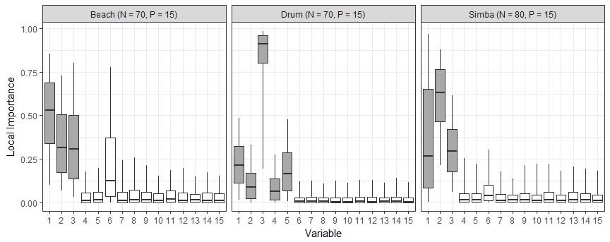
SOLID was able to achieve its enhanced performance, not only by permanently removing variables through global variable selection, but by honing in on more promising lower-dimensional subspaces. Figure 6 shows that our proposed measure of local importance successfully captured the locally active variables. Table 2 shows that across all three test functions, SOLID was optimizing over fewer variables than GVS, as defined by the number of variables explored by the $AEI$ function.

We also compared the methods in terms of computational costs. Oracle, which knows the set of globally active variables and does not perform any variable selection, took 1.8 hours to add 25 design points, averaged across all test functions. For every hour that Oracle took to obtain 25 new design points, None took 1.4 hours, GVS took 4.0 hours, and SOLID took 5.3 hours. Although computationally more expensive, if each evaluation of $f$ is expensive, SOLID would still be preferable to GVS and None, since it required fewer evaluations of $f$ to obtain equivalent or better estimates of $\boldsymbol{\chi}$. To see this, we compared the mean improvement value that Oracle achieves after 7 runs with the number of runs the other approaches needed to achieve at least that value (see Figure 5). On the Beach function, SOLID needed 10 runs, whereas GVS required 13, and None required 15. Similar patterns held for the Drum and Simba functions.

As evidenced in Figure 5, the mean improvement value for GVS eventually met (on the Beach and Simba functions) or exceeded (on the Drum function) the value obtained by SOLID. The difference in how these two methods selected inputs at which to evaluate $f$ next could explain this result. By selecting inputs whose values vary in all $p$ globally active dimensions, GVS may be better able to identify truly globally inactive variables and correctly remove them from the design matrix. By removing more globally inactive variables than SOLID, GVS could eventually experience comparable or better mean improvement values. In the first few sequential runs, however, the results favored SOLID.

The Sarcos robot dataset (Vijayakumar and Schaal, 2000) consists of $n=44,484$ observations and $p=21$ input variables, available at www.gaussianprocess.org/gpml/data. The input variables are the positions, velocities, and accelerations of seven different points on a robot arm as it draws a figure eight (Vijayakumar et al., 2005). We transform the inputs such that $\mathbf{x}\in[0,1]^{21}$. The response variable $Y(\mathbf{x})$ is the first of seven joint torque measurements (Parker, 2015). Sequential optimization requires being able to evaluate the response surface at arbitrary input values, but this is not possible with the discrete Sarcos data. Therefore, for illustration purposes, we generated data assuming the true response surface is a kernel smoothed function. For any input $\mathbf{x}$, we have

where $\mathbb{S}=\{1,...,n\}$, $\mathbf{x}_{i}$ are the observed inputs in the Sarcos dataset, and the kernel smoother is $K(\mathbf{x},\mathbf{x}^{\prime})=\text{exp}\{-\sum_{j=1}^{p}h^{-2}(x_{j}-x^{\prime}_{j})^{2}\}$. Based on 5-fold cross-validation minimizing the out-of-sample prediction MSE, the best bandwidth was $h=0.08272$.

With the fields package in R, we randomly selected inputs that led to space-filling designs. We included ten times as many initial design points as dimensions (Loeppky et al., 2009). We considered only $15$ sequential evaluations in this analysis due to the computational demands. Using only the GVS and SOLID approaches, we evaluated the improvement (13) at each run $i\in\{1,...,15\}$. We set $g=0.15$ and $\rho=0.01$ to provide a moderate amount of variable selection, and we set $\delta=0.20$ to emphasize local searches. $\tau^{2}=0.05$. We used the same priors and number of MCMC chains and posterior samples as in Section 5.

We present results for 100 simulated datasets in Figure 7. SOLID achieved greater improvement than GVS over 100 simulated datasets at nearly every run of the sequential design. Comparing overall improvement, SOLID was significantly better than GVS (p-value $<0.001$). SOLID consistently used fewer variables for optimization than GVS. We found that neither method removed any variables based on global variable selection. However, by the final run, SOLID used $15.88$ variables during its optimization and design selection, compared to $21$ for GVS. Figure 7 shows the proportion of datasets with globally and locally active variables at the final run. Of the 21 input variables, SOLID identified several as locally active. At the last run, variables Position 1, Acceleration 1, and Acceleration 4 were identified as locally active in $93\%$, $100\%$, and $96\%$ of the simulated datasets.

When optimizing a function $f(\cdot)$ where each evaluation is expensive, one goal is to obtain the largest $f(\hat{\boldsymbol{\chi}})$ in as few evaluations of $f$ as possible. To that end, we proposed SOLID, a new method that measures local variable importance around $\hat{\boldsymbol{\chi}}$ and uses this information to optimize $f$ in a sequential design. Whereas global variable selection permanently removes globally inactive variables, our local variable selection approach is flexible, adapting to the uncertainty of $\hat{\boldsymbol{\chi}}$. We tailored local variable selection to optimize the search for both the maximizer of the $AEI$ acquisition function and the global maximizer. Rather than exploring the entire $p-$dimensional space, SOLID examines only the locally active variables. In a simulation study, we found that our definition of local importance successfully captured the subset of locally active variables across three test functions. By reducing the optimization dimension global and local variable selection, our SOLID algorithm was able to achieve higher $f(\hat{\boldsymbol{\chi}})$ values compared to the standard methods, for a fixed number of sequential evaluations.

There are several ways that SOLID could be further improved. One reviewer pointed out that the presence of locally active variables could lead to non-stationary behavior in the response surface. Depending on the nature of non-stationarity, this could result in the estimated GP spatial range parameters, which assume a stationary covariance, as poor indicators of a variable’s global importance. It is our intention that any variable that influences $f$ anywhere in the input space be classified as globally active. Using a GP model with a non-stationary covariance function is the next step, though computational costs would increase and our definition of globally active would need to be modified. On the other hand, a non-stationary covariance function may not be necessary. The three test functions in Section 5 exhibit non-stationary behavior, yet the SOLID behaves well and rarely drops a globally active variable. It is also possible that a stationary covariance function would still able to predict $f$ in a subregion near $\boldsymbol{\chi}$, which is one reason why we chose our local selection criterion to be based on prediction comparisons instead of directly inspecting the estimates of the spatial range parameters.

One limitation of SOLID is its required computations to estimate local importance and its utilization of MCMC to estimate $f$. In instances where the underlying function is inexpensive to evaluate, it would be faster to use conventional sequential design approaches. Additionally, for experiments involving, say, more than 50 variables, the MCMC algorithm presented here for global and local variable selection could become excessively slow and other methods would be preferable, such as the random embedding approach (Wang et al., 2016) or by specifying an additive model (Kandasamy et al., 2015). That said, SOLID’s local variable selection could be used for many functions $f$, without needing to know which or how many variables are locally active. An area of future work would be to incorporate aspects of these other methods within the SOLID framework, perhaps to perform fast initial screening.

References

- Bai et al. (2014) Bai, E., Li, K., Zhao, W., and Xu, W. (2014), “Kernel based approaches to local nonlinear non-parametric variable selection,” Automatica, 50, 100–113.
- Berk et al. (2002) Berk, R. A., Bickel, P., Campbell, K., Fovell, R., Keller-McNulty, S., Kelly, E., Linn, R., Park, B., Perelson, A., Rouphail, N., Sacks, J., and Schoenberg, F. (2002), “Workshop on statistical approaches for the evaluation of complex computer models,” Statist. Sci., 17, 173–192.
- Booker et al. (1999) Booker, A. J., Dennis, J. E., Frank, P. D., Serafini, D. B., Torczon, V., and Trosset, M. W. (1999), “A rigorous framework for optimization of expensive functions by surrogates,” Structural optimization, 17, 1–13.
- Brochu et al. (2010) Brochu, E., Cora, V. M., and de Freitas, N. (2010), “A Tutorial on Bayesian Optimization of Expensive Cost Functions, with Application to Active User Modeling and Hierarchical Reinforcement Learning,” arXiv:1012.2599 [cs.LG].
- Byrd et al. (1995) Byrd, R. H., Lu, P., Nocedal, J., and Zhu, C. (1995), “A Limited Memory Algorithm for Bound Constrained Optimization.” SIAM J. Scientific Computing, 16, 1190–1208.
- Chang et al. (2001) Chang, P., Williams, B., Bhalla, K., Belknap, T., Santner, T., Notz, W., and Bartel, D. (2001), “Design and analysis of robust total joint replacements: Finite element model experiments with environmental variables,” Journal of Biomechanical Engineering, 123, 239–246.
- Crombecq et al. (2011) Crombecq, K., Laermans, E., and Dhaene, T. (2011), “Efficient space-filling and non-collapsing sequential design strategies for simulation-based modeling,” European Journal of Operational Research, 214, 683 – 696.
- Djolonga et al. (2013) Djolonga, J., Krause, A., and Cevher, V. (2013), “High-Dimensional Gaussian Process Bandits,” Advances in Neural Information Processing Systems, 26, 1025–1033.
- Gelman et al. (2004) Gelman, A., Carlin, J. B., Stern, H. S., and Rubin, D. B. (2004), Bayesian Data Analysis, Chapman and Hall/CRC, 2nd ed.
- Gramacy and Lee (2012) Gramacy, R. B. and Lee, H. K. H. (2012), “Cases for the nugget in modeling computer experiments,” Statistics and Computing, 22, 713–722.
- Hahn et al. (1994) Hahn, D., Allers, R., and Minkoff, R. (1994), The Lion King, Walt Disney Pictures.
- Hastings (1970) Hastings, W. K. (1970), “Monte Carlo sampling methods using Markov chains and their applications,” Biometrika, 57, 97–109.
- Huang et al. (2006) Huang, D., Allen, T. T., Notz, W. I., and Zeng, N. (2006), “Global Optimization of Stochastic Black-Box Systems via Sequential Kriging Meta-Models,” Journal of Global Optimization, 34, 441–466.
- Jala et al. (2016) Jala, M., Levy-Leduc, C., Éric Moulines, Conil, E., and Wiart, J. (2016), “Sequential Design of Computer Experiments for the Assessment of Fetus Exposure to Electromagnetic Fields,” Technometrics, 58, 30–42.
- Jones et al. (1998) Jones, D. R., Schonlau, M., and Welch, W. J. (1998), “Efficient Global Optimization of Expensive Black-Box Functions,” Journal of Global Optimization, 13, 455–492.
- Joseph and Hung (2008) Joseph, V. R. and Hung, Y. (2008), “Orthogonal-maximin Latin hypercube designs,” Statistica Sinica, 18, 171–186.
- Kandasamy et al. (2015) Kandasamy, K., Schneider, J., and Poczos, B. (2015), “High Dimensional Bayesian Optimisation and Bandits via Additive Models,” arXiv 1503.01673 [stat.ML].
- Kleijnen (2015) Kleijnen, J. P. C. (2015), Design and Analysis of Simulation Experiments, Springer Publishing Company, Incorporated, 2nd ed.
- Kleijnen et al. (2005) Kleijnen, J. P. C., Sanchez, S. M., Lucas, T. W., and Cioppa, T. M. (2005), “State-of-the-Art Review: A User’s Guide to the Brave New World of Designing Simulation Experiments,” INFORMS Journal on Computing, 17, 263–289.
- Linkletter et al. (2006) Linkletter, C., Bingham, D., Hengartner, N. W., Higdon, D., and Ye, K. Q. (2006), “Variable Selection for Gaussian Process Models in Computer Experiments,” Technometrics, 48, 478–490.
- Lizotte et al. (2012) Lizotte, D. J., Greiner, R., and Schuurmans, D. (2012), “An Experimental Methodology for Response Surface Optimization Methods,” J. of Global Optimization, 53, 699–736.
- Loeppky et al. (2009) Loeppky, J. L., Sacks, J., and Welch, W. J. (2009), “Choosing the Sample Size of a Computer Experiment: A Practical Guide,” Technometrics, 51, 366–376.
- Mebane Jr. and Sekhon (2011) Mebane Jr., W. and Sekhon, J. (2011), “Genetic Optimization Using Derivatives: The rgenoud Package for R,” Journal of Statistical Software, Articles, 42, 1–26.
- Močkus (1975) Močkus, J. (1975), “On Bayesian Methods for Seeking the Extremum,” in Optimization Techniques IFIP Technical Conference Novosibirsk July 1–7, 1974, ed. Marchuk, G. I., Berlin, Heidelberg: Springer Berlin Heidelberg, pp. 400–404.
- Myers et al. (2016) Myers, R. H., Anderson-Cook, C. M., and Montgomery, D. C. (2016), Response Surface Methodology : Process and Product Optimization Using Designed Experiments., Wiley Series in Probability and Statistics, Wiley, 4th ed.
- Oakley and O’Hagan (2004) Oakley, J. E. and O’Hagan, A. (2004), “Probabilistic sensitivity analysis of complex models: A Bayesian approach,” Journal of the Royal Statistical Society Series B, 66, 751–769.
- Parker (2015) Parker, R. (2015), “Efficient Computational Methods for Large Spatial Data,” dissertation, North Carolina State University.
- Picheny and Ginsbourger (2014) Picheny, V. and Ginsbourger, D. (2014), “Noisy kriging-based optimization methods: A unified implementation within the DiceOptim package,” Computational Statistics and Data Analysis, 71, 1035–1053.
- Regis (2016) Regis, R. G. (2016), “Trust regions in Kriging-based optimization with expected improvement,” Engineering Optimization, 48, 1037–1059.
- Reich et al. (2009) Reich, B. J., Storlie, C. B., and Bondell, H. D. (2009), “Variable Selection in Bayesian Smoothing Spline ANOVA Models: Application to Deterministic Computer Codes,” Technometrics, 51, 110–120.
- Sacks et al. (1989) Sacks, J., Schiller, S. B., and Welch, W. J. (1989), “Designs for Computer Experiments,” Technometrics, 31, 41–47.
- Santner et al. (2003) Santner, T. J., Williams, B. J., and Notz, W. I. (2003), The Design and Analysis of Computer Experiments, Springer.
- Shan and Wang (2010) Shan, S. and Wang, G. G. (2010), “Survey of modeling and optimization strategies to solve high-dimensional design problems with computationally-expensive black-box functions,” Structural and Multidisciplinary Optimization, 41, 219–241.
- Vijayakumar et al. (2005) Vijayakumar, S., D’Souza, A., and Schaal, S. (2005), “Incremental Online Learning in High Dimensions,” Neural Computation, 17, 2602–2634.
- Vijayakumar and Schaal (2000) Vijayakumar, S. and Schaal, S. (2000), “Locally Weighted Projection Regression: An O(n) Algorithm for Incremental Real Time Learning in High Dimensional Space,” in in Proceedings of the Seventeenth International Conference on Machine Learning (ICML 2000, pp. 1079–1086.
- Wang et al. (2016) Wang, Z., Hutter, F., Zoghi, M., Matheson, D., and de Freitas, N. (2016), “Bayesian optimization in high dimensions via random embeddings,” Journal of Artificial Intelligence Research, 55, 361–387.
- Welch et al. (1992) Welch, W. J., Buck, R. J., Sacks, J., Wynn, H. P., Mitchell, T. J., and Morris, M. D. (1992), “Screening, Predicting, and Computer Experiments,” Technometrics, 34, 15–25.
- Zhao et al. (2018) Zhao, W., Chen, H.-F., Bai, E.-W., and Li, K. (2018), “Local variable selection of nonlinear nonparametric systems by first order expansion,” Systems & Control Letters, 111, 1–8.
8 Appendix
8.1 MCMC Details
We use Metropolis-Hastings within Gibbs sampling to obtain posterior samples of . For convenience, we reparameterize to the total precision (inverse variance), , and proportion of variance from the response surface, . Using the parameterization in Section 2.2, let
- Hastings (1970) Wilfred Keith Hastings. Monte carlo sampling methods using markov chains and their applications. Biometrika, 57:97–109, 1970.
- Kleijnen (2015) Jack P. C. Kleijnen. Design and Analysis of Simulation Experiments. Springer Publishing Company, Incorporated, 2nd edition, 2015. ISBN 08848289, 97803319180878.
- Rosen (1960) J. B. Rosen. The gradient projection method for nonlinear programming. part I. linear constraints. 8(1):181–217, March 1960. ISSN 0368-4245 (print), 1095-712X (electronic).