Urban contact structures for epidemic simulations: Correcting biases in data-driven approaches
Abstract
Epidemics are emergent phenomena depending on the epidemiological characteristics of pathogens and the interaction and movement of people. Public transit systems have provided much important information about the movement of people, but there are also other means of transportation (e.g., bicycle and private car), that are invisible to public transit data. This discrepancy can induce a bias in disease models that leads to mispredictions of epidemic growth (e.g., peak prevalence and time). In our study, we aim to advance and compare the epidemic spreading dynamics using public transit trips, in contrast to more accurate estimates of population movement using mobile phones traces. In our study, we simulate epidemic outbreaks in a cohort of two million mobile phone users. We use a metapopulation model incorporating susceptible-infected-recovered dynamics to analyze and compare different effective contract matrices, constructed by the public transit systems and mobile phones respectively, on the process of epidemics. We find that epidemic outbreaks using public transit trips tend to be underestimated in terms of the epidemic spreading dynamics, reaching epidemic peaks weaker and later. This is rooted in a later introduction of new infectious people into uninfected locations.
Introduction
Despite the advances in medicine and technology, outbreaks of infectious diseases continue to occur, causing substantial losses in both economy and human health. For example, in 2014, the Ebola epidemic spreading across Guinea, Liberia, and Sierra Leone, greatly impacted the societies and economies of West Africa [1]. In addition to 28,639 cases and 11,316 deaths, the economic loss is estimated to be as high as USD 2.2 billion in 2015 GDP, leaving a declining agricultural production and decreasing cross-border trade [2, 3, 4, 5]. To relieve epidemic risks and reduce socio-economic losses, public health officials seek model-based analyses to inform infectious disease threats (such as the size and time of the outbreak peak) and efficient response strategies to contain and mitigate emerging outbreaks [6].
Population movement and connectivity exacerbate epidemic transmission, deciding the fate of the propagation of the epidemics [7, 8] and the efficacy of public health control measures [9, 10, 11]. An appropriate example would be the spread of 2009 H1N1 pandemic in Mexico City [12, 13, 14, 15]. Epidemic spreading does not only depend on the transmission mechanisms of the pathogens in question but also population movements. To get a high-resolution picture of population movements, many technologies have been used to obtain people’s trajectories through their digital footprints. In contrast with individual explosive electronic records available in public transit systems, the position tracking via mobile phones can track nearly total population movements (e.g. by foot, bicycle, and public transit) and give a more precise description of population movements during an epidemic [16]. It is however more sensitive from a privacy perspective, which is a reason to keep public transportation data as a source for epidemic modeling.
Fine-grained records of public transit are available in many cities, with public access (e.g., Chicago [17] or Chinese cities such as Chongqing and Shanghai soda.datashanghai.gov.cn, accessed April 2, 2018). There is a decades-old line of research in the epidemiological literature to use this data as a proxy for analyzing the features of population movement [18, 19, 20, 21, 22, 23]. However, public transit systems can only track part of movements, dominant in long distance trips. For example, from a study about travel within Shanghai, people tend to travel via public transit for a trip within one hour, but with car for longer journeys [24]. Another Chinese study observed that trips within one kilometer were typically by foot, while people used public transportation for longer trips [25].
In this work, we aim to advance and compare the epidemic spreading dynamics using population movements captured by different position tracking technologies (e.g. mobile phone [26, 27] and public transit [28, 29]). The epidemic outbreaks are introduced into an urban network of locations, driven by population turnover in metapopulations at the location. The metapopulation dynamics follows a susceptible-infected-recovered model [30].
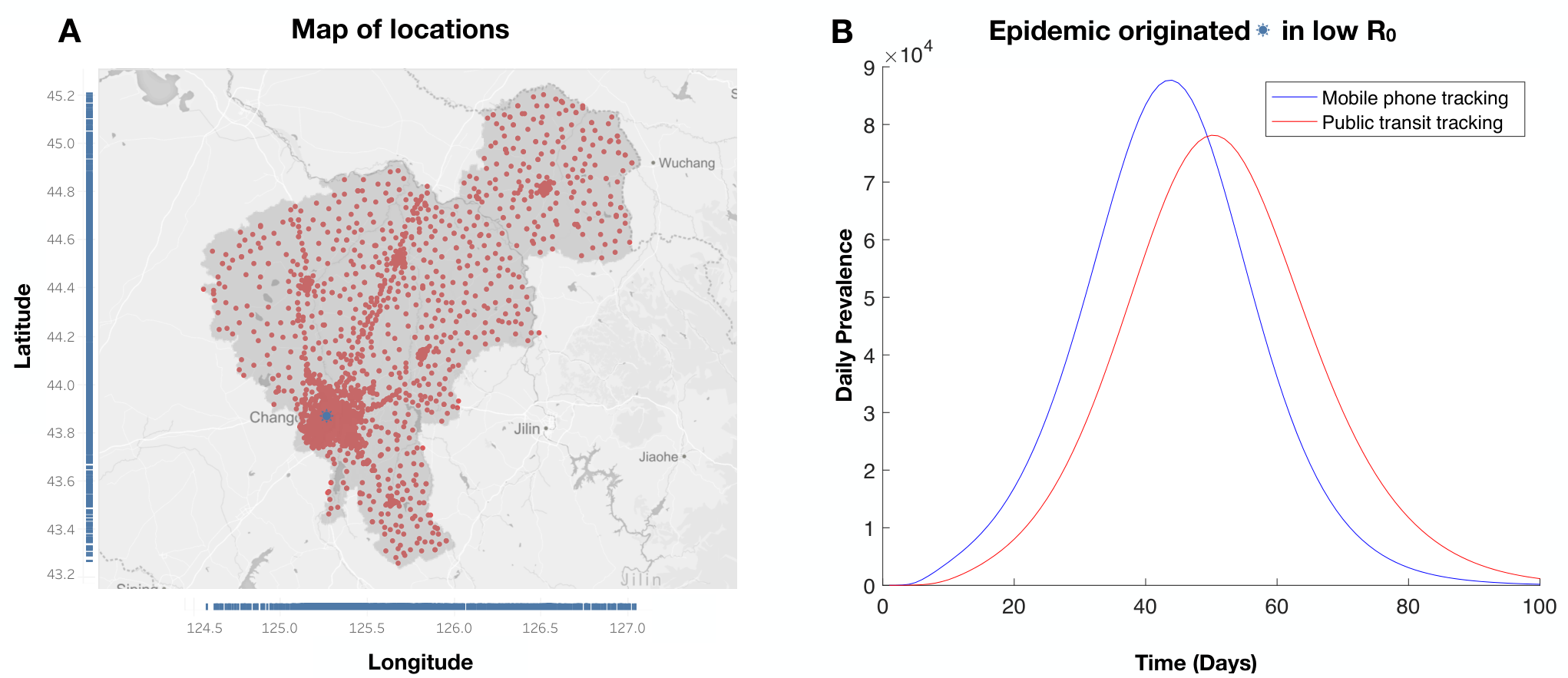
The population movements collected connect over two million mobile phone uses of the eight million inhabitants over one day in Changchun, China in 2017. As we do not have access to public transportation data from Changchun, we use a model to generate such. This model assumes a gamma distribution of trip distances [31]. We track simulated epidemics spreading in epidemiological settings similar to the 2009 Hong Kong H1N1 influenza and 2010 Taiwan varicella epidemics [32], as well as other infectious diseases. We assume the pathogen is introduced in a location probabilistically with respect to its population and follow the time evolution of prevalence for the different ways of tracking the populations. In Fig. 1, we show our proposed analysis methods schematically.
Methods
In this section, we will introduce the epidemic model, how we deal with movement trips, and prevalence measures in the following subsections. We summarize information about parameters in Table 1.
Epidemic model
The millions of inhabitants of a metropolis make individual-based epidemic models challenging [33]. Still one would want to include the location and temporal features of a city in the calculation. One solution, and the one we take, is to represent locations as metapopulations. We base our simulations on the work of Wesolowski et al. [34]. We divide the population into three disease compartments: susceptible (individuals don’t have but could get the disease), infective (individuals who have the disease and can spread it further) and recovered (individuals who are immune or deceased and cannot get or spread the disease). For each location , the number of individuals in the three compartments at time are denoted by , and , respectively. In an entirely susceptible population at location , a new outbreak happens with probability:
| (1) |
where represents the transmission rate; is the population flow (i.e., the number of people traveling during one time unit) from location to location ; and is the fraction of the infected population at day at location
| (2) |
Then we simulate a stochastic process introducing infections into completely susceptible metapopulations. is a Bernoulli random variable with probability .
In locations with infections, the dynamics is deterministic:
| (3) | |||||
| (4) | |||||
| (5) |
where denotes the recovery rate. An important parameter for the discussion is the basic reproduction number, . It is defined as and can be interpreted as the expected number of secondary infections. More specifically, if an infectious individual joins into a susceptible metapopulation. Everyone in such location has an equal probability to contract with other.
| Parameters | Meaning | Range |
|---|---|---|
| number of susceptible individuals at time in location | ||
| number of infective individuals at time in location | ||
| number of recovered individuals at time in location | ||
| transmission rate | [0.5, 15] | |
| recovery rate | [1/5,1] | |
| number of trips from location to location in a day | ||
| population of location | ||
| contact matrix using mobile phone trips | ||
| public transit average traveling distance | [10,50] | |
| public transit mode share | 0.3 | |
| shape parameter in the gamma distribution with respect to | [1,50] | |
| scale parameter in the gamma distribution with respect to | [1,50] | |
| trip distance | ||
| gamma probability distribution, , of public transit trips along with distances | ||
| scale parameter to derive the ratio of public transit trips with respect to | ||
| contact matrix using public transit trips |
Contact network
The compartmental model described above is not the only component of an epidemic simulation. We also need to input the contact patterns, which is used to describe who that is in contact with whom. In this section, we describe how we construct the contact matrices that describe the flow of people between the locations within our example city—Changchun, China.
Trips inferred by mobile phone data
The dataset contains the movements of total of 6,305,500 anonymized mobile phone users in Changchun City during a one-day period on July 3, 2017 (Monday). Fig. S1 shows the temporal number of changing trips in a day. We use a subset of over 2,035,700 anonymized mobile phone users, who only move within the studied city of Changchun. Changchun is the provincial capital and largest city of the Jilin Province. This city had (in 2010) a total population of 7,674,439 under its jurisdiction and an area of 20,604 . In total, the data comprise 3,789 cellular base stations (henceforth locations).
From the movement traces of these users, we construct hourly time series of locations, assuming one individual can only be associated to one location (i.e. the one of longest duration) per hour. At the same time, we construct the contact matrix , where the entry means the number of trips from location to location , by aggregating 24 hourly movements of all users. The population of location , , is assumed to be , where are the number of local trips within the location .
Public transit trips
Even though, as mentioned, several metropolitan regions publish detailed data about public transport trips, Changchun does not (at the moment of writing). Note that, there is a sufficient amount of statistics about the city and the intra city travel for us to reconstruct the contact matrix.
We use some different attributes to model public transit trips and extract the distribution feature of trips: First, the average travel distance by public transit, , is determined. In the city of Changchun, the average speed of public transit is expected to be kilometers per hour in morning and evening rush periods in 2017 [35]. In our analysis, we investigate of three levels to denote traveling trips for to hours: low is defined as in the range of 10–20 kilometers, mediate as 30–40 kilometers and high as 50–60 kilometers. Next quantity we measure is the public transit mode share. Another attribute is the public transit mode share, denoted —the fraction of public transit trips. According to the survey in Changchun urban area [25], the public transit mode share is estimated between 0.3 and 0.4. As thus we set as 0.35 in this study.
To generate public transit trips with accurate and , we use a realistic probability distribution of public transit trips of distance . We assume follows the gamma distribution—. Effectively, dominates the shape whereas dominates the scale. To understand the effect of on , we use gamma distributions with mean value as . We scan the integer values of the parameter space of from two to fifty and from one to fifty. For example, consider the low , then we choose all pairs of and , giving a mean of between 10 and 20. Totally, there are 29 pairs of -values for low , 37 pairs for mediate , and 34 pairs for high . For each , is introduced explicitly to scale the probability when deriving the fraction of public transit trips as . Finally, a trip is labeled as public transit with the probability of . By aggregating public transit trips, we can construct the contact matrix of public transit trips, the same process as that of mobile phone trips.
Simulation setup and analysis
As epidemic outbreaks emerge, their transmission dynamics can vary substantially across the geographical locations of the initial infection in large populations[7, 8], which have been used to model epidemics in urban settings [18, 7, 36]. We make 100 runs for averages. Each run starting from a location chosen with a probability proportional to its population. The outbreaks are characterized by three parameters (the transmission rate , the recovery , and the the average traveling distance ): indicates the probability of a susceptible individual infected in a contact by an infectious individual. ’s inverse gives an expected duration of the infectious state. Finally, parameterizes the public transit behavior of individuals. Simulations with parameter settings of infectious diseases are studied: 2009 Hong Kong H1N1 influenza ( and ) and 2010 Taiwan varicella ( and ) [32], as well as a series of hypothetic infectious diseases. We simulate the hypothetic diseases by three levels of transmission rates (low , mediate , high and ) [34]. For example of a set of parameter settings (i.e., , and low ), there are 29 pairs of and with respect to low . For each pair of and , we run stochastic simulations 30 times using sampled public transit trips. With simulations, we assess these simulated prevalence time-series with respect to the following four comparisons:
- •
- •
Peak timing: The time lag, as , between the prevalence with public transit trips reaching its epidemic peak at time and the prevalence with mobile phone trips reaching its epidemic peak at time at time [36].
- •
Peak magnitude: The ratio, as , of peak prevalence with public transit trips and that with mobile phone trips [36].
- •
Situational awareness: The complement of the normalized mean absolute error (MAE) between prevalences of simulations using public transit trips and that using mobile phone trips, minimized over possible lags [36], given by:
(6) Here, and are the prevalence in simulations using public transit trips and that using mobile phone trips at time , respectively; is the time lag.
To track the epidemic growth rate of new infections in previous susceptible locations, we consider the dynamic percentage of infected locations over time:
- •
Timing of #% locations infected: The time lag as , between the prevalence with public transit reaching #% locations infected at time and that with mobile phones.
Results
Evaluation of prevalence time-series
As mentioned, we scan the - parameter space. A typical epidemic starts with an initial infection at a random location. Except the outbreak size, the epidemic growth can be additionally different. Considering an epidemic as shown in Fig. 2, prevalences using public transit trips are increasing with time, with the peak at the 50 day and end at the 170 day, in contrast, that using mobile phone trips peak at the 40 day.
The epidemic spread is closely tracked in epidemiological settings of 2009 Hong Kong H1N1 influenza ( and ) and 2010 Taiwan varicella ( and ) [32], as well as a series of synthetic, hypothetical infections. Infections of disease outbreaks in urban settings may be detected in one day [34]. We further track the epidemic spread of synthetic infectious diseases over transmission rates (low , mediate , and high ).
Figs. 3 and 4 show the deviations of the simulations based on transit data from the mobile phone based reference. The consistently negative times, shows that both the peak times and early warning times always happens later in the simulations based on public transit data. The small peak magnitudes and situational awarenesses also shows a discrepancy between the outbreaks estimated from the public transit trips and mobile phone trips. In general, one can regard the bias as coming from that the simulations based on the public transit trips are more strongly affected by both and the average traveling distance . For example of low , when , the peak time of prevalence using public transit data is on average at the 17 day, and that using mobile phone at the the 15 day. As thus, the peak timing, as the deviation of their peak times, is on average two days. When , the peak time of prevalence using public transit data is on average at the 48 day, and that using mobile phone at the the 44 day. The peak timing increases to an average of four days (Fig. 3A, 3B and 3C).
Theoretical network analysis
To better understand our observations, we investigate the difference in population flow as predicted by public transit and mobile phone data, respectively. Suppose that an entirely infected location of size is connected to an entirely susceptible location of size . Considering this simple scenario, we can follow the network analysis of Ref. [39] to understand this effect of contact matrices on epidemics. The probability , that the disease is transmitted between an infected individual from the location go to the location, is given by:
| (7) |
Where denotes the movement flow as the number of trips from location to location per time—the entry of contact matrix . Thus the probability that at least one infected individual of location due to location is given:
| (8) |
When is small, the probability can be linear with the term of . As thus, , as the probability of new infections introduced in an entirely susceptible location, correlates positively with and movement flow .
For an infectious disease with fixed , comparing with the contact matrix of mobile phone trips, the contact matrix of public transit trips, with the entry of , is scaled by and has different probability distributions. For example of mediate as 30–40 kilometers (Fig.S3), 95% trips tracked by mobile phone are covered by a range from 0 to 153 kilometers. In contrast, 95% public transit data has a more narrow range (i.e. from 0 to 84 kilometers), only about half of the mobile phone data. These differences contribute to the disparity of probability to infect new locations in epidemic outbreaks.
Furthermore, we evaluate the kind deviation of epidemic prediction between the two types of movement data by considering the expected first time of #% locations being infected. In Fig. 5, we track the spread of realistic infectious diseases (Fig. 3) and hypothetic infectious diseases (Fig. 4). Negative times shows the slower epidemic growths using public transit trips. In general, times are decreasing with increasing and public transit average traveling distance . For example, at the beginning, simulations with public transit trips arrive around when 20% locations new infected later or earlier. With continued epidemics, these simulations will arrive the time of 80% locations new infected later totally.
Conclusions
In computational epidemiology, a common proxy for population flow within cities is public transit data. In this work, we compared such an approach with arguably more realistic data for population movement obtained from mobile phone locations. Simulating outbreaks in several (realistic and hypothetical) scenarios, we found deviations depending on the type of population movement data we input. In the simulations based on public transit data, the peaks of outbreaks tended to arrive later and be weaker. For example, for H1N1 to spread over a medium traveling distance (30–40 kilometers), prevalences using public transit have can have five days delay and be 8% less of the peak when using cell phone data.
We trace the observed effect to a delayed spreading of new infections in totally susceptible locations. New infections driven by public transit data tend to arrive late at an entirely susceptible population, especially for locations with a long distance, due to the significantly reducing number of trips and appearance probability of long trips. We conclude that deviations of epidemic prevalence using public transit decreased with increasing and public transit average traveling distance . This conclusion, in general, could prove useful to public health policymakers, especially when there are only public transit information, and can guide future tracking strategies to infer population movements. It also implies that some earlier literature needs to be re-evaluated. For example of the epidemic risk relied on the public transit data in Tokyo [21], with the public transit mode share as 57% [40], the risk that a single infection causes Tokyo epidemic may be underestimated. With a low transmission rate as and a high work population as , the previous low probability of urban epidemic can be middle or even high, and the peak time can arrive weeks earlier than the estimated two months.
Our work agrees with Ref. [33] in that we need a holistic picture of movements within a city. Future studies along this line can either increase the precision in the population density and flow modeling [41], introduce demographic data [42, 33], or scale up the modeling to the entire humanity [43, 23].
Supporting information
ZW would like to acknowledge funding from the Models of Infectious Disease Agent Study (MIDAS) program grant number U01 GM087719. This work was also funded by the National Natural Science Foundation of China (NSFC) (Grant No. 61772230 and 61402379). The funders had no role in study design, data collection and analysis, decision to publish, or preparation of the manuscript.
| 3946 | 1099422 | 1d | 15285 | 0.89 |
References
- [1] Centers for Disease Control and Prevention. Cost of the ebola epidemic (2017). URL https://www.cdc.gov/vhf/ebola/outbreaks/2014-west-africa/cost-of-ebola.html.
- [2] The World Bank. Gdp growth (annual %) (2014). URL {http://data.worldbank.org/indicator/NY.GDP.MKTP.KD.ZG}.
- [3] The World Bank. Summary on the ebola recovery plan: Sierra leone (2015). URL http://www.worldbank.org/en/topic/ebola/brief/summary-on-the-ebola-recovery-plan-sierra-leone.
- [4] The World Bank. Summary on the ebola recovery plan: Guinea (2015). URL http://www.worldbank.org/en/topic/ebola/brief/summary-on-the-ebola-recovery-plan-sierra-leone.
- [5] The World Bank. Summary on the ebola recovery plan: Liberia - economic stabilization and recovery plan (esrp) (2015). URL {http://www.worldbank.org/en/topic/ebola/brief/summary-on-the-ebola-recovery-plan-liberia-economic-stabilization-and-recovery-plan-esrp}.
- [6] Giesecke, J. Modern infectious disease epidemiology (CRC Press, London, 2017), 3 edn.
- [7] Dalziel, B. D., Pourbohloul, B. & Ellner, S. P. Human mobility patterns predict divergent epidemic dynamics among cities. Proceedings of the Royal Society of London B: Biological Sciences 280, 20130763 (2013).
- [8] Eubank, S. et al. Modelling disease outbreaks in realistic urban social networks. Nature 429, 180–184 (2004).
- [9] Dye, C. & Gay, N. Modeling the sars epidemic. Science 300, 1884–1885 (2003).
- [10] Riley, S. et al. Transmission dynamics of the etiological agent of sars in hong kong: impact of public health interventions. Science 300, 1961–1966 (2003).
- [11] Meyers, L. A., Pourbohloul, B., Newman, M. E. J., Skowronski, D. M. & Brunham, R. C. Network theory and sars: predicting outbreak diversity. Journal of theoretical biology 232, 71–81 (2005).
- [12] Dimitrov, N., Goll, S., Meyers, L. A., Pourbohloul, B. & Hupert, N. Optimizing tactics for use of the US antiviral strategic national stockpile for pandemic (H1N1) influenza, 2009. PLoS Currents 1 (2009).
- [13] Pourbohloul, B. et al. Initial human transmission dynamics of the pandemic (h1n1) 2009 virus in north america. Influenza and other respiratory viruses 3, 215–222 (2009).
- [14] Merler, S., Ajelli, M., Pugliese, A. & Ferguson, N. M. Determinants of the spatiotemporal dynamics of the 2009 h1n1 pandemic in europe: implications for real-time modelling. PLoS Comput Biol 7, e1002205 (2011).
- [15] Xia, S., Liu, J. & Cheung, W. Identifying the relative priorities of subpopulations for containing infectious disease spread. PloS ONE 8, e65271 (2013).
- [16] Frias Martinez, E., Williamson, G. & Frias Martinez, V. An agent-based model of epidemic spread using human mobility and social network information. In Privacy, security, risk and trust (PASSAT) and IEEE third inernational conference on social computing (SocialCom), 57–64 (2011).
- [17] Lee, M. & Holme, P. Relating land use and human intra-city mobility. PLoS ONE 10, e0140152 (2015).
- [18] Cooley, P. et al. The role of subway travel in an influenza epidemic: a new york city simulation. Journal of Urban Health 88, 982 (2011).
- [19] Zhao, B. et al. A preliminary study on spatial spread risk of epidemics by analyzing the urban subway mobility data. Journal of Biosciences and Medicines 3, 15 (2015).
- [20] Zhang, M., Meng, R. & Verbraeck, A. Including public transportation into a large-scale agent-based model for epidemic prediction and control. In Proceedings of the Conference on Summer Computer Simulation, 1–8 (Society for Computer Simulation International, 2015).
- [21] Yashima, K. & Sasaki, A. Epidemic process over the commute network in a metropolitan area. PloS one 9, e98518 (2014).
- [22] Saito, M. M. et al. Enhancement of collective immunity in tokyo metropolitan area by selective vaccination against an emerging influenza pandemic. PloS one 8, e72866 (2013).
- [23] Colizza, V., Barrat, A., Barthelemy, M., Valleron, A.-J. & Vespignani, A. Modeling the worldwide spread of pandemic influenza: baseline case and containment interventions. PLoS Medicine 4, e13 (2007).
- [24] Wang, W.-J. & Gan, H.-C. Car or public transit? Analysis on travel mode choice behavior. Urban Transport of China 3, 011 (2010).
- [25] Wang, H. Analysis on residents’ short-distance travel mode selection based on sp survey—examples of resident behavior in changchun city. ChengShi Jianshe LiLun Yan Jiu 1202–1203 (2014).
- [26] Yan, X.-Y., Zhao, C., Fan, Y., Di, Z. & Wang, W.-X. Universal predictability of mobility patterns in cities. Journal of The Royal Society Interface 11, 20140834 (2014).
- [27] Bengtsson, L. et al. Using mobile phone data to predict the spatial spread of cholera. Scientific reports 5, 8923 (2015).
- [28] Du, Z., Yang, B. & Liu, J. Understanding the spatial and temporal activity patterns of subway mobility flows. arXiv preprint arXiv:1702.02456 (2017).
- [29] Sun, L., Jin, J. G., Axhausen, K. W., Lee, D.-H. & Cebrian, M. Quantifying long-term evolution of intra-urban spatial interactions. J. R. Soc. 12, 20141089 (2015).
- [30] Colizza, V. & Vespignani, A. Epidemic modeling in metapopulation systems with heterogeneous coupling pattern: Theory and simulations. Journal of theoretical biology 251, 450–467 (2008).
- [31] Mazloumi, E., Currie, G. & Rose, G. Using gps data to gain insight into public transport travel time variability. Journal of Transportation Engineering 136, 623–631 (2009).
- [32] Yang, B., Pei, H., Chen, H., Liu, J. & Xia, S. Characterizing and discovering spatiotemporal social contact patterns for healthcare. IEEE Transactions on Pattern Analysis and Machine Intelligence 39, 1532–1546 (2017).
- [33] Mei, S. et al. Simulating city-level airborne infectious diseases. Computers, Environment and Urban Systems 51, 97 – 105 (2015).
- [34] Wesolowski, A. et al. Multinational patterns of seasonal asymmetry in human movement influence infectious disease dynamics. Nature Communications 8, 2069 (2017).
- [35] Changchun city transport department. Work program to be a public transit city (2015-2018) (2018). URL {http://www.cctraffic.com.cn/bus_urban_workplan.jsp}. Online; accessed March 19, 2018.
- [36] Herrera, J. L., Srinivasan, R., Brownstein, J. S., Galvani, A. P. & Meyers, L. A. Disease surveillance on complex social networks. PLoS Computational Biology 12, e1004928 (2016).
- [37] Thompson, W. W., Comanor, L. & Shay, D. K. Epidemiology of seasonal influenza: use of surveillance data and statistical models to estimate the burden of disease. Journal of Infectious Diseases 194, S82–S91 (2006).
- [38] Rath, T. M., Carreras, M. & Sebastiani, P. Automated detection of influenza epidemics with hidden markov models. In International Symposium on Intelligent Data Analysis, 521–532 (Springer, 2003).
- [39] Caillaud, D., Craft, M. E. & Meyers, L. A. Epidemiological effects of group size variation in social species. Journal of The Royal Society Interface 10, 20130206 (2013).
- [40] Goldschein, E. Take a look at why the tokyo metro is known as commuter hell (2014). URL {http://www.businessinsider.com/}. Online; accessed March 19, 2018.
- [41] The spatial organization of the population density in cities (2018). E-print arXiv:1804.00855.
- [42] Chen, J. et al. The effect of demographic and spatial variability on epidemics: A comparison between Beijing, Delhi, and Los Angeles. In Critical Infrastructure (CRIS), 2010 5th International Conference on, 1–8 (IEEE, 2010).
- [43] Balcan, D. et al. Modeling the spatial spread of infectious diseases: The global epidemic and mobility computational model. Journal of computational science 1, 132–145 (2010).
- [44] Clauset, A., Newman, M. E. J. & Moore, C. Finding community structure in very large networks. Phys. Rev. E 70, 066111 (2004). DOI 10.1103/PhysRevE.70.066111.