Effective field theory of the Higgs Mode in a two dimensional dilute Bose gas

Ji-Chong Yang Affiliation: Department of Physics & State Key Laboratory of Surface Physics, Fudan University,
Shanghai 200433, China Affiliation: Department of Physics, Liaoning Normal University, Dalian 116029, China Yu Shi Email: yushi@fudan.edu.cn Thanks: Corresponding author Affiliation: Department of Physics & State Key Laboratory of Surface Physics, Fudan University,
Shanghai 200433, China

Abstract

We investigate the spectral function of the Higgs mode in a two dimensional Bose gas, by using the effective field theory in the zero temperature limit. Our approach explains the experimental feature that the peak of the spectral function is a soft continuum rather than a sharp peak, broadened and vanishing in the superfluid phase, which cannot be explained in terms of the $O(2)$ model. We also find that the scalar susceptibility is the same as the longitudinal susceptibility.

Keywords:

Higgs mode, Bose gas, effective field theory

pacs

05.30.Jp, 74.20.De, 74.25.nd

I Introduction

In condensed matter physics, the Higgs mode was first explored in superconductivity [1], and has recently been observed in ultra-cold Bosons in both three and two dimensional optical lattices [2, 3]. Higgs modes in various other systems have also been studied [4]. The Higgs mode in Boson systems in an optical lattice has been theoretically studied by using $O(2)$ model [5, 6, 7, 8, 9, 10]. However, it was found experimentally that the dependence of the response function on the frequency exhibits a broad continuum rather than a sharp peak [3, 10]. This feature cannot be explained in terms of the $O(2)$ model [6, 7, 8]. Moreover, as the system deviates from the critical point and enters the superfluid phase, the response function broadens and vanishes [3]. This phenomenon also exists in Fermi superfluid [11].

In this paper, we study the spectral function of the Higgs mode in $2+1$ dimensions by using the effective field theory (EFT) in the zero temperature limit [12, 13, 14]. We study the spectral functions of both the longitudinal and the scalar susceptibilities, which are found to be the same when ${\bf q}=0$ . We also find that the feature of the peak of the spectral function is consistent with the experiment. The peak of the longitudinal susceptibility is soft, as observed in the experiment. Furthermore, our theory reproduces the disappearance of the Higgs mode in the ordered phase, as observed in the experiment.

The rest of the paper is organized as the following. In Sec. II, we briefly introduce the EFT in a two dimensional Bose gas. The correlation functions of the Higgs mode are calculated in Sec. III. In Sec. IV, we present the numerical study. Sec. V is a summary.

II Effective field theory

In imaginary time representation, the action of EFT can be written as [14]

\begin{split}&S[\psi^{*},\psi]=\int_{0}^{\beta}d\tau\int d^{D}x\left\{\psi^{*}\left[\frac{\partial}{\partial\tau}-\nabla^{2}-r\right]\psi+\frac{1}{2}g(\psi^{*}\psi)^{2}\right.\\ &\left.+\frac{1}{2}h[\nabla(\psi^{*}\psi)]^{2}+\frac{g_{3}}{36}(\psi^{*}\psi)^{3}+\ldots\right\},\end{split}

(1)

where $r=\mu$ is the chemical potential, $g$ , $h$ , and $g_{3}$ are coupling constants that can be determined from fitting the results with the experimental data, “ $\ldots$ ” represents the higher order terms. We consider only the leading order, that is, the case that $g$ is the only nonzero coupling constant.

One can compare the EFT with the $O(2)$ model, which is a relativistic model and can describe the Bose gas at the vicinity of the critical point, with the action

\begin{split}&S[\Phi]=\int d^{D+1}x\left\{\frac{1}{2}\left(\partial_{\mu}\Phi\right)^{2}-\frac{m^{2}}{2}\Phi^{2}+\frac{U}{4}\Phi^{2}\Phi^{2}\right\},\end{split}

(2)

where $\Phi$ is a two component vector. In EFT, if we write $\psi$ as a two component vector, the only difference with the $O(2)$ model is the derivative with respect to $t$ . Similar to the parametrization of $O(2)$ model, $\psi$ can be parameterized as

\begin{split}&\psi=v+\frac{1}{\sqrt{2}}\left(\psi_{1}+i\psi_{2}\right).\\ \end{split}

(3)

Then the action of effective field theory can be written as

\begin{split}&S[v,\psi_{1},\psi_{2}]=S_{v}[v]+S_{\rm free}[v,\psi_{1},\psi_{2}]+S_{\rm int}[v,\psi_{1},\psi_{2}],\\ &S_{v}[v]=\int d\tau\int d^{d}x\left[-rv^{2}+\frac{1}{2}gv^{4}\right],\\ &S_{\rm free}[v,\psi_{1},\psi_{2}]=\int d\tau\int d^{d}x\left[\frac{i}{2}\left(\psi_{1}\dot{\psi_{2}}-\dot{\psi}_{1}\psi_{2}\right)+\frac{1}{2}\psi_{1}(-\nabla^{2}+X)\psi_{1}+\frac{1}{2}\psi_{2}(-\nabla^{2}+Y)\psi_{2}\right],\\ &S_{\rm int}[v,\psi_{1},\psi_{2}]=\int d\tau\int d^{d}x\left[-\sqrt{2}(\mu-gv^{2})v\psi_{1}+\frac{gv}{\sqrt{2}}\psi_{1}(\psi_{1}^{2}+\psi_{2}^{2})+\frac{1}{8}g(\psi_{1}^{2}+\psi_{2}^{2})^{2}\right],\\ &X=-r+3gv^{2},\;Y=-r+gv^{2}.\\ \end{split}

(4)

II.1 Feynman rules

The lowest-energy classical configuration of the potential is a constant field $\psi=v$ , with

\begin{split}&v=\sqrt{\frac{r}{g}}.\end{split}

(5)

By choosing such a minimum, the global $U(1)$ gauge symmetry is spontaneously broken.

There are ultra violet (UV) divergences in 1-loop calculation in $1+2$ dimensions. One can deal with the UV divergences by renormalization, i.e. rescaling the field as $\psi\to Z^{\frac{1}{2}}\psi$ and introducing the counter terms defined as [15]

\begin{split}&\delta_{z}=Z-1,\;\;\delta_{r}=r_{0}Z-r,\;\;\delta_{g}=g_{0}Z-g.\\ \end{split}

(6)

where $r_{0}$ and $g_{0}$ are bare chemical potential and bare coupling constant, respectively, to replace $r$ and $g$ in the original Lagrangian. We find that $\delta_{g}$ is sufficient to cancel the UV divergence showing up in 1-loop calculation. Thus we use $Z=1$ , $\delta_{z}=\delta_{r}=0$ . With only one counter term, we need only one renormalization condition. Similar to the $O(2)$ model, we use the renormalization condition [6, 8, 15]

\begin{split}&\langle\psi_{1}\rangle=0.\\ \end{split}

(7)

The action at classical minimum with counter terms can be written as

\begin{split}&S[v,\psi_{1},\psi_{2}]=S_{v}[v]+S_{\rm free}[v,\psi_{1},\psi_{2}]+S_{\rm int}[v,\psi_{1},\psi_{2}]+S_{c}[v,\psi_{1},\psi_{2}]\\ &S_{v}[v]=\int d\tau\int d^{d}x\left[\frac{1}{2}(\delta_{g}-g)v^{4}\right],\\ &S_{\rm free}[v,\psi_{1},\psi_{2}]=\int d\tau\int d^{d}x\left[\frac{i}{2}\left(\psi_{1}\dot{\psi}_{2}-\dot{\psi}_{1}\psi_{2}\right)-\frac{1}{2}\psi_{1}(\nabla^{2}-2gv^{2})\psi_{1}-\frac{1}{2}\psi_{2}(\nabla^{2})\psi_{2}\right],\\ &S_{\rm int}[v,\psi_{1},\psi_{2}]=\int d\tau\int d^{d}x\left[\frac{gv}{\sqrt{2}}\psi_{1}(\psi_{1}^{2}+\psi_{2}^{2})+\frac{1}{8}g(\psi_{1}^{2}+\psi_{2}^{2})^{2}\right],\\ &S_{c}[v,\psi_{1},\psi_{2}]=\int d\tau\int d^{d}x\left[\frac{3}{2}\delta_{g}v^{2}\psi_{1}^{2}+\frac{1}{2}\delta_{g}v^{2}\psi_{2}^{2}+\sqrt{2}\delta_{g}v^{3}\psi_{1}+\frac{\delta_{g}v}{\sqrt{2}}\psi_{1}(\psi_{1}^{2}+\psi_{2}^{2})+\frac{\delta_{g}}{8}(\psi_{1}^{2}+\psi_{2}^{2})^{2}\right].\\ \end{split}

(8)

The propagator can be written as [14]

\begin{split}&D(\omega,{\bf p})=\frac{1}{\omega^{2}+\epsilon^{2}(p)}\left(\begin{array}[]{cc}p^{2}&\omega\\ -\omega&p^{2}+2gv^{2}\end{array}\right),\\ &\epsilon({\bf p})=\sqrt{p^{2}(p^{2}+2gv^{2})},\\ \end{split}

(9)

where we have used a Nambu spinor to denote $\psi_{1}$ and $\psi_{2}$ . The Feynman rules for the vertices are shown in Fig. 1.

Refer to caption — Figure 1: Feynman rules of EFT. The solid line is the propagator of $\psi_{1}$ , the dotted line is the propagator of $\psi_{2}$ .

II.2 Susceptibility

The observable we are interested in is the spectral function of Higgs mode. The spectral function can be defined via dynamic susceptibility as [6, 16]

\begin{split}&\chi_{AB}^{\prime\prime}({\bf q},\omega)={\rm Im}(\chi_{AB}({\bf q},i\omega\to\omega+i0^{+})),\end{split}

(10)

so that $\chi_{AB}^{\prime\prime}({\bf q},\omega)$ are the imaginary parts of retarded correlation functions, which can be obtained from thermal correlation functions $\chi_{AB}({\bf q},i\omega)$ by analytical continuation $i\omega\to\omega+i0^{+}$ . The thermal correlation function $\chi_{AB}({\bf q},i\omega)$ can be calculated in imaginary time representation.

The scalar susceptibility is introduced in Ref. [6]. It was argued that to observe the Higgs mode in experiments, one should try to measure the spectral function of the scalar susceptibility. The scalar susceptibility can be associated with the parameterization [14]

\begin{split}&\psi(x,t)=\sqrt{n(x,t)}e^{i\phi(x,t)},\;\;n(x,t)=v^{2}+\rho(x,t).\\ \end{split}

(11)

Using Eq. (3), we find

\begin{split}&\rho(x,t)=\sqrt{2}v\psi_{1}+\frac{1}{2}\psi_{1}^{2}+\frac{1}{2}\psi_{2}^{2}.\\ \end{split}

(12)

Similar to the approach in Ref. [6], it is found that

\begin{split}&\chi_{\rho\rho}=2v^{2}\chi_{\psi_{1}\psi_{1}}+\sqrt{2}v\left(\chi_{\psi_{1}\psi_{1}^{2}}+\chi_{\psi_{1}\psi_{2}^{2}}\right)+\frac{1}{4}\left(\chi_{\psi_{1}^{2}\psi_{1}^{2}}+\chi_{\psi_{2}^{2}\psi_{2}^{2}}+2\chi_{\psi_{1}^{2}\psi_{2}^{2}}\right).\end{split}

(13)

In this paper, we study the spectral functions of both longitudinal susceptibility $\chi^{\prime\prime}_{\psi_{1}\psi_{1}}$ and scalar susceptibility $\chi^{\prime\prime}_{\rho\rho}$ .

III Calculation of correlation functions

Throughout this paper, we consider zero temperature limit and $2+1$ dimensions. We use dimensional regulation (DR) [17] to regulate the UV divergence. For simplicity, in $D=2-\epsilon$ dimensions, we define $N_{\rm UV}$ as

\begin{split}&N_{\rm UV}\equiv\frac{2}{\epsilon}-\gamma_{E}+\log(16\pi)+\log\frac{M^{2}}{2gv^{2}},\end{split}

(14)

where $\gamma_{E}$ is the Euler constant, $M$ is renormalization scale.

III.1 1-loop level

III.1.1 Counter terms at 1-loop order

The renormalization condition in Eq. (7) requires the 1-particle-irreducible (1PI) tadpole diagrams of $\psi_{1}$ vanish. All the 1PI diagrams at 1-loop level are shown in Fig. 2. The diagrams shown in Fig. 2. (a), (b) and (c) are denoted as $I_{a}^{t}$ , $I_{b}^{t}$ and $I_{c}^{t}$ respectively, and can be written as

\begin{split}&I_{a}^{t}=-gv\frac{6}{\sqrt{2}}f_{a}^{t},\;\;\;\;I_{b}^{t}=-gv\frac{2}{\sqrt{2}}f_{b}^{t},\;\;\;\;I_{c}^{t}=-\sqrt{2}\delta_{g}^{(1)}v^{3},\\ \end{split}

(15)

where we use the superscript of $\delta_{g}^{(1)}$ to denote $\delta_{g}$ at 1-loop level, $f_{a}^{t}$ and $f_{b}^{t}$ are obtained in Eq. (62). Using the renormalization condition

\begin{split}&\langle\psi_{1}\rangle=I_{a}^{t}+I_{b}^{t}+I_{c}^{t}=0,\\ \end{split}

(16)

we find that in $D=2-\epsilon$ dimensions, the counter term at 1-loop level can be written as

\begin{split}&\delta_{g}^{(1)}=\frac{g^{2}}{8\pi}\left(N_{\rm UV}-2\right),\\ \end{split}

(17)

where $N_{\rm UV}$ is defined in Eq. (14).

III.1.2 1PI contribution to self-energy at 1-loop order

The 1PI contribution to self-energy of $\psi_{1}$ is denoted as $\Pi_{11}$ . The diagrams contributing to $\Pi_{11}$ at 1-loop level are shown in Fig. 3. The diagrams shown in Fig. 3. (a), (b), (c), (d), (e), (f) and (g) are denoted as $I_{a}^{\psi_{1}}$ , $I_{b}^{\psi_{1}}$ , $I_{c}^{\psi_{1}}$ , $I_{d}^{\psi_{1}}$ , $I_{e}^{\psi_{1}}$ , $I_{f}^{\psi_{1}}$ and $I_{g}^{\psi_{1}}$ , respectively, and can be written as

\begin{split}&I_{a}^{\psi_{1}}=-3gf_{a}^{t},\;\;\;\;I_{b}^{\psi_{1}}=-gf_{b}^{t},\;\;\;\;I_{c}^{\psi_{1}}(\omega_{q},q^{2})=18g^{2}v^{2}f_{a}^{p}(\omega_{q},q^{2}),\\ &I_{d}^{\psi_{1}}(\omega_{q},q^{2})=2g^{2}v^{2}f_{b}^{p}(\omega_{q},q^{2}),\;\;I_{e}^{\psi_{1}}(\omega_{q},q^{2})=I_{f}^{\psi_{1}}(\omega_{q},q^{2})=6g^{2}v^{2}f_{c}^{p}(\omega_{q},q^{2}),\;\;I_{g}^{\psi_{1}}=-3\delta_{g},\\ \end{split}

(18)

where $f_{a}^{t}$ , $f_{b}^{t}$ , $f_{a}^{p}(q^{2})$ , $f_{b}^{p}(q^{2})$ and $f_{c}^{p}(q^{2})$ are given in Eqs. (62), (79), (80) and (73). $\delta_{g}$ are given in Eq. (17). We find

\begin{split}&\Pi_{11}(\omega_{q},q^{2})=\sum_{n=a,\ldots,g}I_{n}^{\psi_{1}}=\frac{g^{2}v^{2}\left(-\frac{\left(\omega_{q}^{2}-20g^{2}v^{4}\right)\sec^{-1}\left(\frac{2gv^{2}}{\omega_{q}}\right)}{\sqrt{4g^{2}v^{4}-\omega_{q}^{2}}}-4\pi gv^{2}+2\omega_{q}\right)}{4\pi\omega_{q}}\\ &-\frac{g^{3}q^{2}v^{4}}{4\pi\omega_{q}^{3}\left(4g^{2}v^{4}-\omega_{q}^{2}\right)^{3/2}}\left(\sqrt{4g^{2}v^{4}-\omega_{q}^{2}}\left(104\pi g^{3}v^{6}-100g^{2}\omega_{q}v^{4}-26\pi g\omega_{q}^{2}v^{2}+21\omega_{q}^{3}\right)\right.\\ &\left.-4\left(100g^{4}v^{8}-37g^{2}\omega_{q}^{2}v^{4}+2\omega_{q}^{4}\right)\sec^{-1}\left(\frac{2gv^{2}}{\omega_{q}}\right)\right)+\mathcal{O}(q^{4}).\end{split}

(19)

The 1PI contribution to self-energy of $\psi_{2}$ is denoted as $\Pi_{22}$ , The diagrams contributing to $\Pi_{22}$ at 1-loop level are shown in Fig. 4. The diagrams shown in Fig. 4. (a), (b), (c), (d) and (e) are denoted as $I_{a}^{\psi_{2}}$ , $I_{b}^{\psi_{2}}$ , $I_{c}^{\psi_{2}}$ , $I_{d}^{\psi_{2}}$ , and $I_{e}^{\psi_{2}}$ respectively, and can be written as

\begin{split}&I_{a}^{\psi_{2}}=-gf_{a}^{t},\;\;\;\;I_{b}^{\psi_{2}}=-3gf_{b}^{t},\;\;\;\;I_{c}^{\psi_{2}}(\omega_{q},q^{2})=2g^{2}v^{2}f_{d}^{p}(\omega_{q},q^{2}),\\ &I_{d}^{\psi_{2}}(\omega_{q},q^{2})=2g^{2}v^{2}f_{e}^{p}(\omega_{q},q^{2}),\;\;\;\;I_{e}^{\psi_{2}}=-\delta_{g}v^{2},\\ \end{split}

(20)

where $f_{e}^{p}(q^{2})=-2f_{c}^{p}(q^{2})$ , $f_{a}^{t}$ , $f_{b}^{t}$ , $f_{c}^{p}(q^{2})$ and $f_{d}^{p}(q^{2})$ are given in Eqs. (62), (73) and (81), while $\delta_{g}$ is given in Eq. (17). We find

\begin{split}&\Pi_{22}(\omega_{q},q^{2})=\sum_{n=a,\ldots,e}I_{n}^{\psi_{2}}=-\frac{g^{2}\omega_{q}v^{2}\sec^{-1}\left(\frac{2gv^{2}}{\omega_{q}}\right)}{4\pi\sqrt{4g^{2}v^{4}-\omega_{q}^{2}}}\\ &+\frac{g^{3}q^{2}v^{4}\left(4g^{2}v^{4}\sqrt{4g^{2}v^{4}-\omega_{q}^{2}}\sec^{-1}\left(\frac{2gv^{2}}{\omega_{q}}\right)-4g^{2}\omega_{q}v^{4}+\omega_{q}^{3}\right)}{4\pi\omega_{q}\left(\omega_{q}^{2}-4g^{2}v^{4}\right)^{2}}+\mathcal{O}(q^{4}).\\ \end{split}

(21)

The 1PI contribution to self-energy that one $\psi_{1}$ is annihilated while a $\psi_{2}$ is created is denoted as $\Pi_{12}$ . The diagrams contributing to $\Pi_{12}$ at 1-loop level are shown in Fig. 5. The diagrams shown in Fig. 5. (a) (b) and (c) are denoted as $I_{a}^{\psi_{1}\psi_{2}}$ , $I_{b}^{\psi_{1}\psi_{2}}$ and $I_{c}^{\psi_{1}\psi_{2}}$ respectively, and can be written as

\begin{split}&I_{a}^{\psi_{1}\psi_{2}}=0,\;\;\;\;I_{b}^{\psi_{1}\psi_{2}}(\omega_{q},q^{2})=6g^{2}v^{2}f_{f}^{p}(\omega_{q},q^{2}),\;\;\;\;I_{c}^{\psi_{1}\psi_{2}}(\omega_{q},q^{2})=-2g^{2}v^{2}f_{g}^{p}(\omega_{q},q^{2}),\\ \end{split}

(22)

where $f_{f}^{p}(q^{2})$ and $f_{p}^{p}(q^{2})$ are given in Eqs. (82) and (83). We find

\begin{split}&\Pi_{12}(\omega_{q},q^{2})=I_{b}^{\psi_{1}\psi_{2}}(\omega_{q},q^{2})+I_{c}^{\psi_{1}\psi_{2}}(\omega_{q},q^{2})=\frac{g^{3}v^{4}\sec^{-1}\left(\frac{2gv^{2}}{\omega_{q}}\right)}{\pi\sqrt{4g^{2}v^{4}-\omega_{q}^{2}}}-\frac{g^{2}v^{2}}{8}\\ &-\frac{g^{2}q^{2}v^{2}}{8\pi\omega_{q}^{2}\left(4g^{2}v^{4}-\omega_{q}^{2}\right)^{3/2}}\left(\sqrt{4g^{2}v^{4}-\omega_{q}^{2}}\left(32\pi g^{3}v^{6}-28g^{2}\omega_{q}v^{4}-8\pi g\omega_{q}^{2}v^{2}+5\omega_{q}^{3}\right)\right.\\ &\left.-4\left(28g^{4}v^{8}-13g^{2}\omega_{q}^{2}v^{4}+\omega_{q}^{4}\right)\sec^{-1}\left(\frac{2gv^{2}}{\omega_{q}}\right)\right)+\mathcal{O}(q^{4}).\end{split}

(23)

III.1.3 1PI contribution to cross susceptibilities

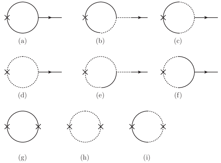
The cross susceptibilities at 1-loop level are denoted as $\chi_{\psi_{1}^{2}\psi_{1}}^{(1)}$ , $\chi_{\psi_{2}^{2}\psi_{1}}^{(1)}$ , $\chi_{\psi_{1}^{2}\psi_{1}^{2}}^{(1)}$ , $\chi_{\psi_{2}^{2}\psi_{2}^{2}}^{(1)}$ and $\chi_{\psi_{1}^{2}\psi_{2}^{2}}^{(1)}$ , where we use the superscript to denote the susceptibilities at 1-loop level. The 1PI diagrams contributing to cross susceptibilities at 1-loop level are shown in Fig. 6. The diagrams shown in Fig. 6. (a), (b), (c), (d), (e), (f), (g), (h) and (i) are denoted as $I_{a}^{cs}$ , $I_{b}^{cs}$ , $I_{c}^{cs}$ , $I_{d}^{cs}$ , $I_{e}^{cs}$ , $I_{f}^{cs}$ , $I_{g}^{cs}$ , $I_{h}^{cs}$ and $I_{i}^{cs}$ respectively, and can be written as

\begin{split}&I_{a}^{ct}(\omega_{q},q^{2})=-2\frac{6gv}{\sqrt{2}}f_{a}^{p}(\omega_{q},q^{2})\frac{q^{2}}{\omega_{q}^{2}+\epsilon^{2}(q)},\;I_{b}^{ct}(\omega_{q},q^{2})=-2\frac{2gv}{\sqrt{2}}f_{f}^{p}(\omega_{q},q^{2})\frac{\omega_{q}}{\omega_{q}^{2}+\epsilon^{2}(q)},\\ &I_{c}^{ct}(\omega_{q},q^{2})=-2\frac{2gv}{\sqrt{2}}f_{c}^{p}(\omega_{q},q^{2})\frac{q^{2}}{\omega_{q}^{2}+\epsilon^{2}(q)},\;I_{d}^{ct}(\omega_{q},q^{2})=-2\frac{2gv}{\sqrt{2}}f_{b}^{p}(\omega_{q},q^{2})\frac{q^{2}}{\omega_{q}^{2}+\epsilon^{2}(q)},\\ &I_{e}^{ct}(\omega_{q},q^{2})=2\frac{2gv}{\sqrt{2}}f_{g}^{p}(\omega_{q},q^{2})\frac{\omega_{q}}{\omega_{q}^{2}+\epsilon^{2}(q)},\;I_{f}^{ct}(\omega_{q},q^{2})=-2\frac{6gv}{\sqrt{2}}f_{c}^{p}(\omega_{q},q^{2})\frac{q^{2}}{\omega_{q}^{2}+\epsilon^{2}(q)},\\ &I_{g}^{ct}(\omega_{q},q^{2})=4f_{a}^{p}(\omega_{q},q^{2}),\;\;\;\;I_{h}^{ct}(\omega_{q},q^{2})=4f_{b}^{p}(\omega_{q},q^{2}),\;\;\;\;I_{i}^{ct}(\omega_{q},q^{2})=4f_{c}^{p}(\omega_{q},q^{2}).\\ \end{split}

(24)

We find at 1-loop level that

\begin{split}&\chi_{\psi_{1}^{2}\psi_{1}}^{(1)}(\omega_{q},{\bf q})+\chi_{\psi_{2}^{2}\psi_{1}}^{(1)}(\omega_{q},{\bf q})=\sum_{n=a,\ldots,f}I_{n}^{ct}(\omega_{q},q^{2})\\ &=-\frac{g^{2}v^{3}\sec^{-1}\left(\frac{2gv^{2}}{\omega_{q}}\right)}{\pi\omega_{q}\sqrt{8g^{2}v^{4}-2\omega_{q}^{2}}}+\frac{q^{2}g^{2}v^{3}}{2\pi\omega_{q}^{3}\sqrt{8g^{2}v^{4}-2\omega_{q}^{2}}\left(2gq^{2}v^{2}+q^{4}+\omega_{q}^{2}\right)\left(\omega_{q}^{2}-4g^{2}v^{4}\right)}\\ &\times\left\{4\left(\omega_{q}^{2}-3g^{2}v^{4}\right)\left(\omega_{q}^{2}\left(q^{2}-2gv^{2}\right)-12g^{2}q^{2}v^{4}\right)\sec^{-1}\left(\frac{2gv^{2}}{\omega_{q}}\right)+\sqrt{4g^{2}v^{4}-\omega_{q}^{2}}\left[-40\pi g^{3}q^{2}v^{6}\right.\right.\\ &\left.\left.+4g^{2}v^{4}\omega_{q}\left(9q^{2}-2\pi\omega_{q}\right)+2gv^{2}\omega_{q}^{2}\left(5\pi q^{2}+\omega_{q}\right)+\omega_{q}^{3}\left(2\pi\omega_{q}-7q^{2}\right)\right]\right\}+\mathcal{O}(q^{4}),\\ &\chi_{\psi_{1}^{2}\psi_{1}^{2}}^{(1)}(\omega_{q},{\bf q})+\chi_{\psi_{2}^{2}\psi_{2}^{2}}^{(1)}(\omega_{q},{\bf q})+2\chi_{\psi_{1}^{2}\psi_{2}^{2}}^{(1)}(\omega_{q},{\bf q})=I_{g}^{ct}(\omega_{q},q^{2})+I_{h}^{ct}(\omega_{q},q^{2})+2I_{i}^{ct}(\omega_{q},q^{2})\\ &=\frac{2g^{2}v^{4}\sec^{-1}\left(\frac{2gv^{2}}{\omega_{q}}\right)}{\pi\omega_{q}\sqrt{4g^{2}v^{4}-\omega_{q}^{2}}}-\frac{gq^{2}v^{2}}{\pi\omega_{q}^{3}\left(4g^{2}v^{4}-\omega_{q}^{2}\right)^{3/2}}\left(8g^{2}v^{4}\left(\omega_{q}^{2}-3g^{2}v^{4}\right)\sec^{-1}\left(\frac{2gv^{2}}{\omega_{q}}\right)\right.\\ &\left.+\left(8\pi g^{3}v^{6}-6g^{2}\omega_{q}v^{4}-2\pi g\omega_{q}^{2}v^{2}+\omega_{q}^{3}\right)\sqrt{4g^{2}v^{4}-\omega_{q}^{2}}\right)+\mathcal{O}(q^{4}).\end{split}

(25)

At 1-loop level, the self energy can be written as

\begin{split}&\Sigma^{(1)}(\omega_{q},q^{2})=D_{0}(\omega_{q},{\bf q})+D_{0}(\omega_{q},{\bf q})\cdot\Pi\cdot D_{0}(\omega_{q},{\bf q})\end{split}

(26)

where $D(\omega_{q},q^{2})$ is defined in Eq. (9), while $\Pi(\omega_{q},q^{2})$ is defined as

\begin{split}&\Pi(\omega_{q},q^{2})\equiv\left(\begin{array}[]{cc}\Pi_{11}(\omega_{q},q^{2})&-\Pi_{12}(\omega_{q},q^{2})\\ \Pi_{12}(\omega_{q},q^{2})&\Pi_{22}(\omega_{q},q^{2})\end{array}\right),\\ \end{split}

(27)

The thermal correlation function $\chi^{(1)}_{\psi_{1}\psi_{1}}$ at 1-loop level is the matrix element $\left(\Sigma^{(1)}(\omega_{q},q^{2})\right)^{11}$ at 1-loop level. One can find that there is an infrared singularity in $\chi_{\psi_{1}\psi_{1}}$ when $\omega_{q}\to 0$ and ${\bf q}=0$ . However, for scalar susceptibility, such an infrared singularity is cancelled, as in the $O(2)$ model [6]. Using Eq. (13), we find that

\begin{split}&\chi^{(1)}_{\rho\rho}(\omega_{q},{\bf q})=\frac{q^{2}\left(gv^{2}+8\pi v^{2}\right)}{4\pi\omega_{q}^{2}}+\mathcal{O}(q^{4})\end{split}

(28)

III.2 Higher order contributions

We can sum up all the 1PI contributions to infinite orders, as shown in Fig. 7. The self-energy is denoted as $\Sigma$ , and the 1PI contributions can be written as a matrix, as in Eq. (27).

The equation in Fig. 7 can be written as

\begin{split}&\Sigma(\omega_{q},q^{2})=\sum_{\begin{subarray}{c}n=0\end{subarray}}^{\infty}D(\omega_{q},{\bf q})\cdot\left(\Pi(\omega_{q},q^{2})\cdot D(\omega_{q},{\bf q})\right)^{n}=D(\omega_{q},{\bf q})\cdot\left(I-\Pi(q^{2})\cdot D(\omega_{q},{\bf q})\right)^{-1}\\ &=\left(D(\omega_{q},{\bf q})^{-1}-\Pi(\omega_{q},q^{2})\right)^{-1},\end{split}

(29)

where $I$ is the identity matrix, $D(\omega_{q},q^{2})$ is defined in Eq. (9). Eq. (29) is the well-known Dyson equation. For simplicity, we only give the result at ${\bf q}=0$ , which can be written as

\begin{split}&\Sigma(\omega_{q},q^{2})\equiv\left(\begin{array}[]{cc}\Sigma_{11}(\omega_{q},q^{2})&\Sigma_{21}(\omega_{q},q^{2})\\ \Sigma_{12}(\omega_{q},q^{2})&\Sigma_{22}(\omega_{q},q^{2})\end{array}\right),\end{split}

(30)

with

\begin{split}&\Sigma_{11}(\omega_{q},q^{2}=0)=16\pi g^{2}v^{2}\omega_{q}\sec^{-1}\left(\frac{2gv^{2}}{\omega_{q}}\right)/\left[\pi^{2}\left(g^{2}v^{2}+8\omega_{q}\right){}^{2}\sqrt{4g^{2}v^{4}-\omega_{q}^{2}}\right.\\ &\left.-4g^{3}v^{4}\sec^{-1}\left(\frac{2gv^{2}}{\omega_{q}}\right)\left(g\sqrt{4g^{2}v^{4}-\omega_{q}^{2}}\sec^{-1}\left(\frac{2gv^{2}}{\omega_{q}}\right)+2(g+12\pi)\omega_{q}\right)\right],\end{split}

(31)

\begin{split}&\Sigma_{22}(\omega_{q},q^{2}=0)=\frac{16\pi gv^{2}}{\omega_{q}}\times\left\{\left[2\sqrt{4g^{2}v^{4}-\omega_{q}^{2}}\left(2\pi g^{2}v^{2}-g\omega_{q}+4\pi\omega_{q}\right)\right.\right.\\ &\left.\left.+g\left(\omega_{q}^{2}-20g^{2}v^{4}\right)\sec^{-1}\left(\frac{2gv^{2}}{\omega_{q}}\right)\right]/\left[\pi^{2}\left(g^{2}v^{2}+8\omega_{q}\right){}^{2}\sqrt{4g^{2}v^{4}-\omega_{q}^{2}}\right.\right.\\ &\left.\left.-4g^{3}v^{4}\sec^{-1}\left(\frac{2gv^{2}}{\omega_{q}}\right)\left(g\sqrt{4g^{2}v^{4}-\omega_{q}^{2}}\sec^{-1}\left(\frac{2gv^{2}}{\omega_{q}}\right)+2(g+12\pi)\omega_{q}\right)\right]\right\},\end{split}

(32)

\begin{split}&\Sigma_{12}(\omega_{q},q^{2}=0)=-\Sigma_{21}(\omega_{q},q^{2}=0)=-8\pi\left[\pi\left(g^{2}v^{2}+8\omega_{q}\right)\sqrt{4g^{2}v^{4}-\omega_{q}^{2}}\right.\\ &\left.-8g^{3}v^{4}\sec^{-1}\left(\frac{2gv^{2}}{\omega_{q}}\right)\right]/\left[\pi^{2}\left(g^{2}v^{2}+8\omega_{q}\right){}^{2}\sqrt{4g^{2}v^{4}-\omega_{q}^{2}}\right.\\ &\left.-4g^{3}v^{4}\sec^{-1}\left(\frac{2gv^{2}}{\omega_{q}}\right)\left(g\sqrt{4g^{2}v^{4}-\omega_{q}^{2}}\sec^{-1}\left(\frac{2gv^{2}}{\omega_{q}}\right)+2(g+12\pi)\omega_{q}\right)\right].\end{split}

(33)

The spectrum $\omega(q)$ can be given as the poles of the self-energy [14],

\begin{split}&\det\left(D(\omega,{\bf q})^{-1}-\Pi(\omega,q)\right)=0.\end{split}

(34)

We find

\begin{split}&\lim_{\omega\to 0}\left[\det\left(D(\omega_{q},{\bf q}=0)^{-1}-\Pi(\omega_{q},q^{2}=0)\right)\right]=0.\\ \end{split}

(35)

which implies that $\omega(q^{2}=0)=0$ is a solution of Eq. (34). Therefore there is no gap in the spectrum of $\psi$ , respecting the Hugenholz-Pines theorem [18].

The correlation function $\chi_{\psi_{1}\psi_{1}}$ can be obtained as

\begin{split}&\chi_{\psi_{1}\psi_{1}}(\omega_{q},{\bf q})=\Sigma_{11}(\omega_{q},q^{2}=0).\end{split}

(36)

The 1PI summation of cross-susceptibilities are shown in Figs. 8 and 9.

The diagrams in Fig. 8 represent

\begin{split}&\chi_{\psi_{1}^{2}\psi_{1}}(\omega_{q},{\bf q})+\chi_{\psi_{2}^{2}\psi_{1}}(\omega_{q},{\bf q})=-2\frac{6gv}{\sqrt{2}}f_{a}^{p}(\omega_{q},q^{2})\Sigma_{11}(\omega_{q},q^{2})-2\frac{2gv}{\sqrt{2}}f_{f}^{p}(\omega_{q},q^{2})\Sigma_{21}(\omega_{q},q^{2})\\ &-2\frac{2gv}{\sqrt{2}}f_{c}^{p}(\omega_{q},q^{2})\Sigma_{11}(\omega_{q},q^{2})-2\frac{2gv}{\sqrt{2}}f_{b}^{p}(\omega_{q},q^{2})\Sigma_{11}(\omega_{q},q^{2})+2\frac{2gv}{\sqrt{2}}f_{g}^{p}(\omega_{q},q^{2})\Sigma_{21}(\omega_{q},q^{2})\\ &-2\frac{6gv}{\sqrt{2}}f_{c}^{p}(\omega_{q},q^{2})\Sigma_{11}(\omega_{q},q^{2}).\\ \end{split}

(37)

The diagrams in Fig. 9 represent

\begin{split}&\chi_{\psi_{1}^{2}\psi_{1}^{2}}(\omega_{q},q^{2})=4f_{a}^{p}(\omega_{q},q^{2})+8g^{2}v^{2}\left(3f_{a}^{p}(\omega_{q},q^{2})+f_{c}^{p}(\omega_{q},q^{2})\right)^{2}\Sigma_{11}(\omega_{q},q^{2})\\ &-8g^{2}v^{2}\left(f_{f}^{p}(\omega_{q},q^{2})\right)^{2}\Sigma_{22}(\omega_{q},q^{2})-16g^{2}v^{2}\left(3f_{a}^{p}(\omega_{q},q^{2})+f_{c}^{p}(\omega_{q},q^{2})\right)f_{f}^{p}(\omega_{q},q^{2})\Sigma_{12}(\omega_{q},q^{2}),\\ &\chi_{\psi_{2}^{2}\psi_{2}^{2}}(\omega_{q},q^{2})=4f_{b}^{p}(\omega_{q},q^{2})+8g^{2}v^{2}\left(f_{b}^{p}(\omega_{q},q^{2})+3f_{c}^{p}(\omega_{q},q^{2})\right)^{2}\Sigma_{11}(\omega_{q},q^{2})\\ &-8g^{2}v^{2}\left(f_{g}^{p}(\omega_{q},q^{2})\right)^{2}\Sigma_{22}(\omega_{q},q^{2})+16g^{2}v^{2}\left(f_{b}^{p}(\omega_{q},q^{2})+3f_{c}^{p}(\omega_{q},q^{2})\right)f_{g}^{p}(\omega_{q},q^{2})\Sigma_{12},\\ &\chi_{\psi_{1}^{2}\psi_{2}^{2}}(\omega_{q},q^{2})=4f_{c}^{p}(\omega_{q},q^{2})+8g^{2}v^{2}\left(f_{c}^{p}(\omega_{q},q^{2})+3f_{a}^{p}(\omega_{q},q^{2})\right)\times\left[\Sigma_{11}(\omega_{q},q^{2})f_{b}^{p}(\omega_{q},q^{2})\right.\\ &\left.+3\Sigma_{11}(\omega_{q},q^{2})f_{c}^{p}(\omega_{q},q^{2})+\Sigma_{12}f_{g}^{p}(\omega_{q},q^{2})\right]+8g^{2}v^{2}f_{f}^{p}(\omega_{q},q^{2})\times\left[\Sigma_{21}(\omega_{q},q^{2})f_{b}^{p}(\omega_{q},q^{2})\right.\\ &\left.+3\Sigma_{21}(\omega_{q},q^{2})f_{c}^{p}(\omega_{q},q^{2})+\Sigma_{22}(\omega_{q},q^{2})f_{g}^{p}(\omega_{q},q^{2})\right].\end{split}

(38)

Using Eqs. (13), (36), (37) and (38), we find

\begin{split}&\chi_{\rho\rho}(\omega_{q},{\bf q}=0)=\left[64\pi g^{2}v^{4}\omega_{q}\sec^{-1}\left(\frac{2gv^{2}}{\omega_{q}}\right)\right]/\left[64\pi^{2}\omega_{q}^{2}\sqrt{4g^{2}v^{4}-\omega_{q}^{2}}\right.\\ &\left.-8g^{2}v^{2}\omega_{q}\left(g(g+12\pi)v^{2}\sec^{-1}\left(\frac{2gv^{2}}{\omega_{q}}\right)-2\pi^{2}\sqrt{4g^{2}v^{4}-\omega_{q}^{2}}\right)\right.\\ &\left.+g^{4}v^{4}\sqrt{4g^{2}v^{4}-\omega_{q}^{2}}\left(\pi^{2}-4\sec^{-1}\left(\frac{2gv^{2}}{\omega_{q}}\right){}^{2}\right)\right].\end{split}

(39)

In experiments, the spectral function is normalized after being measured [3]. We find that after normalization, the spectral functions $\chi^{\prime\prime}_{\psi_{1}\psi_{1}}(\omega_{q},{\bf q}=0)$ and $\chi^{\prime\prime}_{\rho\rho}(\omega_{q},{\bf q}=0)$ are the same as each other. In the rest of the paper, we only concentrate on $\chi^{\prime\prime}_{\psi_{1}\psi_{1}}(\omega_{q},{\bf q}=0)$ .

IV Numerical results

To obtain the numerical results, we need to match the coupling constant $g$ . One can match the coupling constant $g$ at tree level and the leading order of $q^{2}$ , the result is $g=8\pi a_{s}$ [14], where $a_{s}$ is the s-wave scattering length. However, in experiments, the system is tunable via $j\equiv J/U$ , where $J$ is the hopping constant, $U$ is the interaction strength. To obtain the dependence of the parameters on the the hopping constant $J$ , we introduce an action derived from the Bose-Hubbard model by using Hubbard-Stratanovich transformation [19, 20, 21],

\begin{split}&S[\psi^{*},\psi]=\int_{0}^{\beta}d\tau\int d^{D}x\left\{K_{1}\psi^{*}\frac{\partial}{\partial\tau}\psi+K_{2}|\frac{\partial}{\partial\tau}\psi|^{2}+K_{3}|\nabla\psi|^{2}+r|\psi|^{2}+\frac{u}{2}|\psi|^{4}+\mathcal{O}(\psi^{6})\right\},\end{split}

(40)

where

\begin{split}&r=\frac{1}{Za^{d}}\left(\frac{1}{J}-\left(\frac{n_{0}+1}{n_{0}U-\mu}+\frac{n_{0}}{\mu-(n_{0}-1)U}\right)\right),\\ &n_{0}=\left\{\begin{array}[]{cc}0,&\mu/U<0;\\ 1,&0<\mu/U<1;\\ 2,&1<\mu/U<2;\\ \ldots&\end{array}\right.\\ &K_{1}=-\frac{r}{\mu},\\ \end{split}

(41)

where $Z$ is the coordinate number, $a$ is the lattice spacing, $\mu$ is the chemical potential. Comparing Eq. (40) with Eq. (1), one can find that when $K_{2}=0$ , Eq. (40) reduces to Eq. (1), which is the EFT.

Based on the comparison of Eqs. (40) and (41) with Eq. (1), we assume

\begin{split}&r=\alpha\left(\frac{j}{j_{c}}-1\right),\;\;\bar{r}\equiv\frac{r}{\alpha}=\left(\frac{j}{j_{c}}-1\right).\end{split}

(42)

where $\alpha$ is an arbitrary constant parameter with dimension of $m^{2}$ . Then we can use the dimensionless variable

\begin{split}&\bar{\omega}\equiv\frac{\omega_{q}}{\alpha}.\end{split}

(43)

After variable substitution and normalization, $\chi^{\prime\prime}_{\psi_{1}\psi_{1}}$ depends only on the massless parameters $\bar{r}$ , $\bar{\omega_{q}}$ and $g$ . The perturbation works only when $g\ll 1$ , so we choose $g<1$ . The normalized spectral function $\chi^{\prime\prime}_{\psi_{1}\psi_{1}}(\omega_{q},{\bf q}=0)$ is shown in Fig. 10 with the parameter values $\bar{r}=2$ and $g=0.1$ , $g=0.3$ and $g=0.5$ .

We find that the peaks of the spectral functions form broadened continuums rather than sharp peaks, in consistency with the experiment [3]. We also find that similar to $O(2)$ model, when $g$ decreases, the peak becomes sharper. This cannot explain the disappearance of the Higgs mode observed in the experiment [3].

When $\bar{r}\gg\bar{\omega_{q}}$ , the spectral function can be simplified as

\begin{split}&\chi^{\prime\prime}_{\psi_{1}\psi_{1}}(\bar{\omega}_{q},{\bf q}=0)\approx\frac{1}{N}\frac{4\pi g\left(\pi\bar{r}\left(g^{2}\bar{\omega}_{q}+24\pi g\bar{\omega}_{q}+64\pi^{2}\bar{\omega}_{q}\right)-8\bar{\omega}_{q}\left(\pi^{2}g\bar{r}\right)\right)}{\bar{r}\left(\left(g^{2}\bar{\omega}_{q}+24\pi g\bar{\omega}_{q}+64\pi^{2}\bar{\omega}_{q}\right)^{2}+\left(8\pi^{2}g\bar{r}\right)^{2}\right)}\end{split}

(44)

where $N$ is the normalization factor. So we can find the maximum is at

\begin{split}&\bar{\omega}_{q}=\frac{8g\bar{r}\pi^{2}}{g^{2}+24g\pi+64\pi^{2}}\approx\frac{g}{8}\left(\frac{j}{j_{c}}-1\right)\\ \end{split}

(45)

when $\bar{r}\gg\bar{\omega_{q}}$ and $g\ll 1$ .

In the experiment, with the increase of the lattice potential depth, $g$ increases approximately linearly and $J$ decreases exponentially [22]. The spectral function as a function of $j/j_{c}$ , while $g$ is kept constant, is shown in Fig. 11. One canclearly see the peak and the energy gap, as well as the disappearance of the Higgs mode. We find that the spectral function shown in Fig. 11 fits well the observation in the experiment [3].

V Conclusion

The Higgs mode discovered in the 2D optical lattice ended the debate whether the Higgs mode can be observed in the 2D neutral superfluid. However, the feature that the peek is a soft continuum above the gap energy rather than a sharp peak, and the disappearance of the response in the ordered phase, cannot be explained using the $O(2)$ model.

In this paper, we have investigated the spectral function of the Higgs mode by using an EFT model. We calculate the spectral functions of both longitudinal susceptibility $\chi^{\prime\prime}_{\psi_{1}\psi_{1}}$ and scalar susceptibility $\chi^{\prime\prime}_{\rho\rho}$ . The spectral functions are obtained as shown in Eqs. (36) and (39), and are drawn in Fig. 10 and Fig. 11.

We find that the visibility of the Higgs mode is the same in longitudinal and scalar susceptibilities. Our EFT calculation reproduces various experimental features, including the softness of the peak of the spectral function and the disappearance of the response with the increase of $j/j_{c}$ .

This work is supported by National Natural Science Foundation of China (Grant No. 12075059).

Appendix A The results of Feynman diagrams

A.1 Results of some integrals

Similar to Ref. [14], we also use the definition

\begin{split}&I_{m,n}(A^{2})\equiv M^{\epsilon}\int\frac{d^{D}k}{(2\pi)^{D}}\frac{k^{2m}}{k^{n}(k^{2}+A^{2})^{\frac{n}{2}}}=\frac{M^{\epsilon}A^{D+2m-2n}}{(4\pi)^{\frac{D}{2}}}\frac{\Gamma(\frac{D-n}{2}+m)\Gamma(n-m-\frac{D}{2})}{\Gamma(\frac{D}{2})\Gamma(\frac{n}{2})}.\\ \end{split}

(46)

Another integral we need can be defined as

\begin{split}&J_{a,b,c}(A^{2},B^{2})\equiv M^{\epsilon}\int\frac{d^{D}k}{(2\pi)^{D}}\frac{1}{(k^{2})^{a}(k^{2}+A^{2})^{b}(4k^{2}(k^{2}+A^{2})+B^{2})^{c}}.\\ \end{split}

(47)

It can be calculated in Mellin-Barnes representation [23], as

\begin{split}&J_{a,b,c}=\frac{M^{\epsilon}}{2^{2c}2\pi i}\int_{-i\infty}^{i\infty}dz\frac{\Gamma(c+z)\Gamma(-z)}{\Gamma(c)}\int\frac{d^{D}k}{(2\pi)^{D}}\frac{\left(\frac{B^{2}}{4}\right)^{z}}{(k^{2})^{a}(k^{2}+A^{2})^{b}(k^{2}(k^{2}+A^{2}))^{c+z}}.\\ \end{split}

(48)

With the help of $I_{m,n}$ calculated in Eq. (46), it can be written as

\begin{split}&J_{a,b,c}(A^{2},B^{2})=\frac{M^{\epsilon}\left(\frac{A^{2}}{2}\right)^{\frac{D}{2}-a-b-2c}}{2^{2c+1}\Gamma(c)\Gamma(\frac{D}{2})(4\pi)^{\frac{D}{2}}\sqrt{\pi}}\frac{1}{2\pi i}\int_{-i\infty}^{i\infty}dz\left(\frac{B^{2}}{A^{4}}\right)^{z}\\ &\times\frac{\Gamma(c+z)\Gamma(-z)\Gamma(\frac{D}{2}-a-c-z)\Gamma(\frac{a+b}{2}+c-\frac{D}{4}+z)\Gamma(\frac{a+b+1}{2}+c-\frac{D}{4}+z)}{\Gamma(b+c+z)}.\\ \end{split}

(49)

For convenience, we define

\begin{split}&j(a,b,c,d,e)\equiv\frac{1}{2\pi i}\int_{-i\infty}^{i\infty}dz\frac{\Gamma(a+z)\Gamma(b+z)\Gamma(c+z)\Gamma(d-z)\Gamma(-z)}{\Gamma(e+z)}t^{z},\\ \end{split}

(50)

which is calculated by closing the contour of the integral and using

\begin{split}&{\rm Res}(\Gamma(a\pm n),z=\mp(n+a))=\pm\frac{(-1)^{n}}{n!}.\\ \end{split}

(51)

It is obtained that

\begin{split}&j(a,b,c,d,e)=\sum_{n=0}^{\infty}\left(\Gamma(d)\Gamma(1-d)\frac{\Gamma(a+n)\Gamma(b+n)\Gamma(c+n)}{\Gamma(e+n)\Gamma(1-d+n)}\frac{t^{n}}{n!}\right.\\ &\left.+t^{d}\Gamma(-d)\Gamma(1+d)\frac{\Gamma(a+d+n)\Gamma(b+d+n)\Gamma(c+d+n)}{\Gamma(e+d+n)\Gamma(1+d+n)}\frac{t^{n}}{n!}\right),\\ \end{split}

(52)

where we have used the relation

\begin{split}&\Gamma(x-n)=(-1)^{n}\frac{\Gamma(x)\Gamma(1-x)}{\Gamma(1-x+n)},\end{split}

(53)

when $n$ is an integer.

Then using the definition of Hypergeometric function

\begin{split}&\;{}_{p}F_{q}\left(\left.\begin{array}[]{c}a_{1},a_{2},...,a_{p}\\ b_{1},b_{2},...,b_{q}\end{array}\right|x\right)=\sum_{n=0}^{\infty}\frac{\prod_{i=1}^{p}(a_{i})_{n}}{\prod_{j=1}^{q}(b_{j})_{n}}\frac{x^{n}}{n!},\end{split}

(54)

we find

\begin{split}&j(a,b,c,d,e)=\frac{\Gamma(a)\Gamma(b)\Gamma(c)\Gamma(d)}{\Gamma(e)}\;_{3}F_{2}\left(\left.\begin{array}[]{c}a,b,c\\ e,1-d\end{array}\right|t\right)\\ &+t^{d}\frac{\Gamma(a+d)\Gamma(b+d)\Gamma(c+d)\Gamma(-d)}{\Gamma(e+d)}\;_{3}F_{2}\left(\left.\begin{array}[]{c}a+d,b+d,c+d\\ e+d,1+d\end{array}\right|t\right).\\ \end{split}

(55)

With the help of $j(a,b,c,d,e)$ calculated in Eq. (55), $J_{a,b,c}$ can be written as

\begin{split}&J_{a,b,c}=\frac{M^{\epsilon}\left(A^{2}\right)^{\frac{D}{2}-a-b-2c}}{2^{2c}\Gamma(\frac{D}{2})(4\pi)^{\frac{D}{2}}}\\ &\times\left(\frac{\Gamma(a+b+2c-\frac{D}{2})\Gamma(\frac{D}{2}-a-c)}{\Gamma(b+c)}\;_{3}F_{2}\left(\left.\begin{array}[]{c}c,\frac{a+b}{2}+c-\frac{D}{4},\frac{a+b+1}{2}+c-\frac{D}{4}\\ b+c,1+a+c-\frac{D}{2}\end{array}\right|\frac{B^{2}}{A^{4}}\right)\right.\\ &+\left(\frac{B^{2}}{4A^{4}}\right)^{\frac{D}{2}-a-c}\left.\frac{\Gamma(\frac{D}{2}-a)\Gamma(a+c-\frac{D}{2})}{\Gamma(c)}\;_{3}F_{2}\left(\left.\begin{array}[]{c}\frac{D}{2}-a,\frac{b-a}{2}+\frac{D}{4},\frac{b-a+1}{2}+\frac{D}{4}\\ \frac{D}{2}+b-a,1-a-c+\frac{D}{2}\end{array}\right|\frac{B^{2}}{A^{4}}\right)\right).\\ \end{split}

(56)

When using DR to regulate the UV divergences we need to calculate the $\epsilon$ -expansion of the Hypergeometric function which can be written as

\begin{split}&h\equiv\frac{A^{\epsilon}\Gamma(x_{1}+\alpha_{1}\epsilon)\Gamma(\alpha_{2}\epsilon)}{\Gamma(x_{2}+\alpha_{3}\epsilon)\times(x_{3}+\alpha_{4}\epsilon)}\;_{3}F_{2}\left(\left.\begin{array}[]{c}y_{1},y_{2}+\beta_{1}\epsilon,\beta_{2}\epsilon\\ y_{3},y_{4}+\beta_{3}\epsilon\end{array}\right|t\right).\end{split}

(57)

Using the definition Eq. (52), we find

\begin{split}&h=\frac{A^{\epsilon}\Gamma(x_{1}+\alpha_{1}\epsilon)\Gamma(\alpha_{2}\epsilon)}{\Gamma(x_{2}+\alpha_{3}\epsilon)\times(x_{3}+\alpha_{4}\epsilon)}+\frac{A^{\epsilon}\Gamma(x_{1}+\alpha_{1}\epsilon)\Gamma(\alpha_{2}\epsilon)}{\Gamma(x_{2}+\alpha_{3}\epsilon)\times(x_{3}+\alpha_{4}\epsilon)}\sum_{n=1}^{\infty}\frac{\frac{\Gamma(y_{1}+n)}{\Gamma(y_{1})}\frac{\Gamma(y_{2}+\beta_{1}\epsilon+n)}{\Gamma(y_{2}+\beta_{1}\epsilon)}\frac{\Gamma(\beta_{2}\epsilon+n)}{\Gamma(\beta_{2}\epsilon)}}{\frac{\Gamma(y_{3}+n)}{\Gamma(y_{3})}\frac{\Gamma(y_{4}+\beta_{3}\epsilon+n)}{\Gamma(y_{4}+\beta_{3}\epsilon)}}\frac{t^{n}}{n!}.\\ \end{split}

(58)

Then we can expand the Gamma function around $\epsilon\to 0$ in each term and gather the summation, and obtain

\begin{split}&h=\frac{1}{\epsilon}\frac{\Gamma(x_{1})}{\alpha_{2}x_{3}\Gamma(x_{2})}+\frac{\Gamma(x_{1})\left(\log(A)+\alpha_{1}\psi^{(0)}(x_{1})-\alpha_{3}\psi^{(0)}(x_{2})-\gamma_{E}\alpha_{2}\right)}{\alpha_{2}x_{3}\Gamma(x_{2})}-\frac{\alpha_{4}\Gamma(x_{1})}{\alpha_{2}x_{3}^{2}\Gamma(x_{2})}\\ &+t\frac{\beta_{2}\Gamma(x_{1})}{x_{3}\alpha_{2}\Gamma(x_{2})}\sum_{n=0}^{\infty}\Gamma(n+1)\frac{\frac{\Gamma(y_{1}+1+n)}{\Gamma(y_{1})}\frac{\Gamma(y_{2}+1+n)}{\Gamma(y_{2})}}{\frac{\Gamma(y_{3}+1+n)}{\Gamma(y_{3})}\frac{\Gamma(y_{4}+1+n)}{\Gamma(y_{4})}}\frac{t^{n}}{\Gamma(n+2)}+\mathcal{O}(\epsilon)\\ &=\frac{1}{\epsilon}\frac{\Gamma(x_{1})}{\alpha_{2}x_{3}\Gamma(x_{2})}+\frac{\Gamma(x_{1})\left(\log(A)+\alpha_{1}\psi^{(0)}(x_{1})-\alpha_{3}\psi^{(0)}(x_{2})-\gamma_{E}\alpha_{2}\right)}{\alpha_{2}x_{3}\Gamma(x_{2})}-\frac{\alpha_{4}\Gamma(x_{1})}{\alpha_{2}x_{3}^{2}\Gamma(x_{2})}\\ &+t\frac{\beta_{2}\Gamma(x_{1})}{x_{3}\alpha_{2}\Gamma(x_{2})}\frac{\Gamma(y_{3})\Gamma(y_{4})\Gamma(y_{1}+1)\Gamma(y_{2}+1)}{\Gamma(y_{1})\Gamma(y_{2})\Gamma(y_{3}+1)\Gamma(y_{4}+1)}\;_{4}F_{3}\left(\left.\begin{array}[]{c}1,1,y_{1}+1,y_{2}+1\\ 2,y_{3}+1,y_{4}+1\end{array}\right|t\right)+\mathcal{O}(\epsilon).\\ \end{split}

(59)

where $\gamma_{E}$ is the Eular constant, $\psi^{(0)}(x)$ is the digamma function.

A.2 Tadpole diagrams

All the tadpole diagrams at 1-loop level are drawn in Fig. 12. The diagrams in Fig. 12. (a), (b) and (c) are denoted as $f_{a}^{t}$ , $f_{b}^{t}$ and $f_{c}^{t}$ , and can be written as

\begin{split}&f_{a}^{t}=\frac{1}{2}M^{\epsilon}\int\frac{d\omega}{2\pi}\int\frac{d^{D}k}{(2\pi)^{D}}\frac{k^{2}}{\omega^{2}+\epsilon^{2}(k)},\\ &f_{b}^{t}=\frac{1}{2}M^{\epsilon}\int\frac{d\omega}{2\pi}\int\frac{d^{D}k}{(2\pi)^{D}}\frac{k^{2}+2gv^{2}}{\omega^{2}+\epsilon^{2}(k)},\\ &f_{c}^{t}=M^{\epsilon}\int\frac{d\omega}{2\pi}\int\frac{d^{D}k}{(2\pi)^{D}}\frac{\omega}{\omega^{2}+\epsilon^{2}(k)}.\\ \end{split}

(60)

We first integrate over $\omega$ , then express the result in terms of $I_{m,n}$ defined in Eq. (46),

\begin{split}&f_{a}^{t}=\frac{1}{4}I_{1,1}(2gv^{2}),\;\;\;f_{b}^{t}=\frac{1}{4}I_{-1,-1}(2gv^{2}),\;\;\;f_{c}^{t}=0.\\ \end{split}

(61)

In $D=2-\epsilon$ dimensions, using Eq. (46), we find

\begin{split}&f_{a}^{t}=\frac{2gv^{2}}{4}\left(-\frac{N_{\rm UV}}{8\pi}+\frac{1}{8\pi}\right),\;\;\;f_{b}^{t}=\frac{2gv^{2}}{4}\left(\frac{N_{\rm UV}}{8\pi}+\frac{1}{8\pi}\right).\\ \end{split}

(62)

A.3 Polarization diagrams

Other 1-loop diagrams we need are listed in Fig. 13, and the diagrams in Fig. 13. (a), (b), (c), (d), (e), (f) and (c) are denoted as $f_{a}^{p}(q^{2})$ , $f_{b}^{p}(q^{2})$ , $f_{c}^{p}(q^{2})$ , $f_{d}^{p}(q^{2})$ , $f_{e}^{p}(q^{2})$ , $f_{f}^{p}(q^{2})$ and $f_{g}^{p}(q^{2})$ , and can be written as

\begin{split}&f_{a}^{p}(\omega_{q},q^{2})=\frac{1}{2}M^{\epsilon}\int\frac{d\omega}{2\pi}\int\frac{d^{D}k}{(2\pi)^{D}}\frac{k^{2}}{\omega^{2}+\epsilon^{2}(k)}\frac{(k+q)^{2}}{(\omega+\omega_{q})^{2}+\epsilon^{2}(k+q)},\\ &f_{b}^{p}(\omega_{q},q^{2})=\frac{1}{2}M^{\epsilon}\int\frac{d\omega}{2\pi}\int\frac{d^{D}k}{(2\pi)^{D}}\frac{k^{2}+2gv^{2}}{\omega^{2}+\epsilon^{2}(k)}\frac{(k+q)^{2}+2gv^{2}}{(\omega+\omega_{q})^{2}+\epsilon^{2}(k+q)},\\ &f_{c}^{p}(\omega_{q},q^{2})=-\frac{1}{2}M^{\epsilon}\int\frac{d\omega}{2\pi}\int\frac{d^{D}k}{(2\pi)^{D}}\frac{\omega(\omega+\omega_{q})}{(\omega^{2}+\epsilon^{2}(k))((\omega+\omega_{q})^{2}+\epsilon^{2}(k+q))},\\ &f_{d}^{p}(\omega_{q},q^{2})=M^{\epsilon}\int\frac{d\omega}{2\pi}\int\frac{d^{D}k}{(2\pi)^{D}}\frac{k^{2}}{\omega^{2}+\epsilon^{2}(k)}\frac{(k+q)^{2}+2gv^{2}}{(\omega+\omega_{q})^{2}+\epsilon^{2}(k+q)},\\ &f_{e}^{p}(\omega_{q},q^{2})=M^{\epsilon}\int\frac{d\omega}{2\pi}\int\frac{d^{D}k}{(2\pi)^{D}}\frac{\omega(\omega+\omega_{q})}{(\omega^{2}+\epsilon^{2}(k))((\omega+\omega_{q})^{2}+\epsilon^{2}(k+q))}=-2f_{c}^{p}(q^{2}),\\ &f_{f}^{p}(\omega_{q},q^{2})=M^{\epsilon}\int\frac{d\omega}{2\pi}\int\frac{d^{D}k}{(2\pi)^{D}}\frac{k^{2}}{\omega^{2}+\epsilon^{2}(k)}\frac{-(\omega+\omega_{q})}{(\omega+\omega_{q})^{2}+\epsilon^{2}(k+q)},\\ &f_{g}^{p}(\omega_{q},q^{2})=M^{\epsilon}\int\frac{d\omega}{2\pi}\int\frac{d^{D}k}{(2\pi)^{D}}\frac{k^{2}+2gv^{2}}{\omega^{2}+\epsilon^{2}(k)}\frac{-(\omega+\omega_{q})}{(\omega+\omega_{q})^{2}+\epsilon^{2}(k+q)}.\\ \end{split}

(63)

We also calculate those integrals at long wave length limit as in Ref. [14], that is, after integrating over $\omega$ , we expand the result at $q^{2}\to 0$ before integrating over $k$ .

Take $f_{c}^{p}(q^{2})$ as an example, after Feynman parameter, $f_{c}^{p}(q^{2})$ can be written as

\begin{split}&f_{c}^{p}(\omega_{q},q^{2})=-\frac{1}{2}\int_{0}^{1}dx\int\frac{d\omega}{2\pi}\int\frac{d^{D}k}{(2\pi)^{D}}\left(\frac{\omega^{2}+(1-2x)\omega\omega_{q}-x(1-x)\omega_{q}^{2}}{\left(\omega^{2}+x\epsilon^{2}(k+q)+(1-x)\epsilon^{2}(k)+x(1-x)\omega_{q}^{2}\right)^{2}}\right).\\ \end{split}

(64)

The terms with odd powers of $\omega$ do not contribute. Hence the integral can be written as

\begin{split}&f_{c}^{p}(\omega_{q},q^{2})=f_{c_{1}}^{p}+f_{c_{2}}^{p},\\ &f_{c_{1}}^{p}=-\frac{1}{2}\int_{0}^{1}dx\int\frac{d\omega}{2\pi}\int\frac{d^{D}k}{(2\pi)^{D}}\left(\frac{\omega^{2}}{\left(\omega^{2}+x\epsilon^{2}(k+q)+(1-x)\epsilon^{2}(k)+x(1-x)\omega_{q}^{2}\right)^{2}}\right),\\ &I_{c_{2}}^{p}=-\frac{1}{2}\int_{0}^{1}dx\int\frac{d\omega}{2\pi}\int\frac{d^{D}k}{(2\pi)^{D}}\left(\frac{-x(1-x)\omega_{q}^{2}}{\left(\omega^{2}+x\epsilon^{2}(k+q)+(1-x)\epsilon^{2}(k)+x(1-x)\omega_{q}^{2}\right)^{2}}\right).\\ \end{split}

(65)

After integrating over $\omega$ , $f_{c_{1}}^{p}$ can be written as

\begin{split}&f_{c_{1}}^{p}=-\frac{1}{8}\int_{0}^{1}dx\int\frac{d^{D}k}{(2\pi)^{D}}\frac{1}{(x\epsilon^{2}(k+q)+(1-x)\epsilon^{2}(k)+x(1-x)\omega_{q}^{2})^{\frac{1}{2}}}.\\ \end{split}

(66)

By using integration-by-part (IBP) recursive relation [24],

\begin{split}&D\int d^{D}kf(k)+\int d^{D}k\left(k\cdot\frac{\partial}{\partial k}f(k)\right)=0,\\ \end{split}

(67)

we obtain

\begin{split}&f_{c_{1}}^{p}=-\frac{1}{8D}\int_{0}^{1}dx\int\frac{d^{D}k}{(2\pi)^{D}}\frac{1}{(x\epsilon^{2}(k+q)+(1-x)\epsilon^{2}(k)+x(1-x)\omega_{q}^{2})^{\frac{3}{2}}}\\ &\times\left((1-x)\times\left(k^{4}+k^{2}(k^{2}+2gv^{2})\right)+x\times\left(k\cdot(k+q)\left(2(k+q)^{2}+2gv^{2}\right)\right)\right).\\ \end{split}

(68)

Then by integrating over $x$ , we write the result as

\begin{split}&f_{c_{1}}^{p}=-\frac{1}{4D}\int\frac{d^{D}k}{(2\pi)^{D}}\left(\frac{k^{4}+k^{2}(k^{2}+2gv^{2})}{\epsilon(k)\left((\epsilon(k)+\epsilon(k+q))^{2}+\omega_{q}^{2}\right)}\right.\\ &\left.+\frac{k\cdot(k+q)\left(2(k+q)^{2}+2gv^{2}\right)}{\epsilon(k+q)\left((\epsilon(k)+\epsilon(k+q))^{2}+\omega_{q}^{2}\right)}\right).\\ \end{split}

(69)

Then we use the long wavelength approximation, and expand $f_{c_{1}}^{p}$ around $q^{2}\to 0$ , and obtain

\begin{split}&f_{c_{1}}^{p}=-\frac{1}{4D}\left\{2\left[J_{-\frac{3}{2},\frac{1}{2},1}+J_{-\frac{1}{2},-\frac{1}{2},1}\right]+\frac{q^{2}}{2D}\left[(1-D)\omega_{q}^{4}m^{6}J_{\frac{1}{2},\frac{5}{2},3}\right.\right.\\ &\left.\left.-\omega_{q}^{2}m^{4}\left((4-D)\omega_{q}^{2}-4(4D-3)m^{4}\right)J_{-\frac{1}{2},\frac{5}{2},3}\right.\right.\\ &\left.\left.+4\left((3-16D)\omega_{q}^{2}m^{6}+12(2-D)m^{10}\right)J_{-\frac{3}{2},\frac{5}{2},3}\right.\right.\\ &\left.\left.+16\left(-7(1+D)\omega_{q}^{2}m^{4}+(32-17D)m^{8}\right)J_{-\frac{5}{2},\frac{5}{2},3}\right.\right.\\ &\left.\left.+16\left(-(11+16D)\omega_{q}^{2}m^{2}+(66-41D)m^{6}\right)J_{-\frac{7}{2},\frac{5}{2},3}\right.\right.\\ &\left.\left.+16\left(-2(2+D)\omega_{q}^{2}+(76-51D)m^{4}6\right)J_{-\frac{9}{2},\frac{5}{2},3}\right.\right.\\ &\left.\left.+64(13-8D)m^{2}J_{-\frac{11}{2},\frac{5}{2},3}+128(D-2)J_{-\frac{13}{2},\frac{5}{2},3}\right]\right\}+\mathcal{O}(q^{4}).\\ \end{split}

(70)

In above, we have used the relation

\begin{split}&\int d^{D}k(k\cdot q)^{2}=\int d^{D}k\frac{k^{2}q^{2}}{D},\end{split}

(71)

and defined $m^{2}\equiv 2gv^{2}$ for convenience.

Using the same procedure as for $f_{c_{2}}^{p}$ , we find

\begin{split}&f_{c_{2}}^{p}=\frac{\omega_{q}^{2}}{2D}\left\{2\left[J_{-\frac{3}{2},\frac{1}{2},2}+J_{-\frac{1}{2},-\frac{1}{2},2}\right]-\frac{q^{2}}{2D}\left[(D-1)\omega_{q}^{4}m^{6}J_{\frac{1}{2},\frac{5}{2},4}\right.\right.\\ &\left.\left.-\omega_{q}^{2}m^{4}\left((4-D)\omega_{q}^{2}-8(2-3D)m^{4}\right)J_{-\frac{1}{2},\frac{5}{2},4}\right.\right.\\ &\left.\left.-16m^{6}\left(-(7D+1)\omega_{q}^{2}+5(D-3)m^{4}\right)J_{-\frac{3}{2},\frac{5}{2},4}\right.\right.\\ &\left.\left.-8\left(-(32+27D)\omega_{q}^{2}m^{4}+2(90-31D)m^{8}\right)J_{-\frac{5}{2},\frac{5}{2},4}\right.\right.\\ &\left.\left.-16\left(-2(11+6D)\omega_{q}^{2}m^{2}+(223-79D)m^{6}\right)J_{-\frac{7}{2},\frac{5}{2},4}\right.\right.\\ &\left.\left.-16\left(-4(2+D)\omega_{q}^{2}+(300-101D)m^{4}\right)J_{-\frac{9}{2},\frac{5}{2},4}\right.\right.\\ &\left.\left.+128(8D-27)m^{2}J_{-\frac{11}{2},\frac{5}{2},4}+256(D-4)J_{-\frac{13}{2},\frac{5}{2},4}\right]\right\}+\mathcal{O}(q^{4}).\\ \end{split}

(72)

In $D=2-\epsilon$ dimensions, using Eqs. (56) and (56), we find

\begin{split}&f_{c}^{p}(\omega_{q},q^{2})=-\frac{1}{4}\left\{\frac{N_{\rm UV}}{8\pi}-\frac{\omega_{q}\cos^{-1}\left(\frac{\omega_{q}}{m^{2}}\right)}{8\pi\sqrt{m^{4}-\omega_{q}^{2}}}+\frac{q^{2}m^{2}}{16\pi\omega_{q}^{3}\left(m^{4}-\omega_{q}^{2}\right)^{2}}\left[3m^{4}\omega_{q}^{2}\sqrt{m^{4}-\omega_{q}^{2}}\cos^{-1}\left(\frac{\omega_{q}}{m^{2}}\right)\right.\right.\\ &\left.\left.-2m^{8}\sqrt{m^{4}-\omega_{q}^{2}}\cos^{-1}\left(\frac{\omega_{q}}{m^{2}}\right)+\left(m^{4}-\omega_{q}^{2}\right)\left(-2m^{4}\omega_{q}-\pi m^{2}\omega_{q}^{2}+\omega_{q}^{3}+\pi m^{6}\right)\right]\right\}+\mathcal{O}(q^{4}).\\ \end{split}

(73)

The other integrals are simpler, so we do not need to use IBP relation. After integrating over $\omega$ , we can expand the result around $q^{2}\to 0$ and write it in terms of functions $J_{a,b,c}$ . The results are

\begin{split}&f_{a}^{p}(\omega_{q},q^{2})=\frac{1}{4}\left\{2J_{-\frac{3}{2},\frac{1}{2},1}+\frac{q^{2}}{2D}\left[\left((3D-1)\omega_{q}^{4}m^{4}\right)J_{-\frac{1}{2},\frac{5}{2},3}\right.\right.\\ &\left.\left.+\left((5D-4)\omega_{q}^{4}m^{2}-(28-16D)\omega_{q}^{2}m^{6}\right)J_{-\frac{3}{2},\frac{5}{2},3}\right.\right.\\ &\left.\left.+\left(2D\omega_{q}^{4}-(140-32D)\omega_{q}^{2}m^{4}+(16D-32)m^{8}\right)J_{-\frac{5}{2},\frac{5}{2},3}\right.\right.\\ &\left.\left.+\left((16D-160)\omega_{q}^{2}m^{2}+(16D-192)m^{6}\right)J_{-\frac{7}{2},\frac{5}{2},3}\right.\right.\\ &\left.\left.-80Dm^{2}J_{-\frac{9}{2},\frac{5}{2},3}+(64-32D)J_{-\frac{11}{2},\frac{5}{2},3}\right]\right\}+\mathcal{O}\left(q^{4}\right).\\ \end{split}

(74)

\begin{split}&f_{b}^{p}(\omega_{q},q^{2})=\frac{1}{4}\left\{2J_{\frac{1}{2},-\frac{3}{2},1}+\frac{q^{2}}{2D}\left[\left((3-D)\omega_{q}^{4}m^{4}\right)J_{\frac{3}{2},\frac{1}{2},3}\right.\right.\\ &\left.\left.+\left((4+D)\omega_{q}^{4}m^{2}-(16D-36)\omega_{q}^{2}m^{6}\right)J_{\frac{1}{2},\frac{1}{2},3}\right.\right.\\ &\left.\left.+\left(2D\omega_{q}^{4}-(32D-52)\omega_{q}^{2}m^{4}+(160-48D)m^{8}\right)J_{-\frac{1}{2},\frac{1}{2},3}\right.\right.\\ &\left.\left.+\left(-(32+16D)\omega_{q}^{2}m^{2}+(576-176D)m^{6}\right)J_{-\frac{3}{2},\frac{1}{2},3}\right.\right.\\ &\left.\left.+\left(-48\omega_{q}^{2}+(736-240D)m^{4}\right)J_{-\frac{5}{2},\frac{1}{2},3}\right.\right.\\ &\left.\left.+((384-144D)m^{2})J_{-\frac{7}{2},\frac{1}{2},3}+(64-32D)J_{-\frac{9}{2},\frac{1}{2},3}\right]\right\}+\mathcal{O}\left(q^{4}\right).\\ \end{split}

(75)

\begin{split}&f_{d}^{p}(\omega_{q},q^{2})=\frac{1}{2}\left\{2J_{-\frac{1}{2},-\frac{1}{2},1}+\frac{q^{2}}{2D}\left[\left((3-D)\omega_{q}^{4}m^{4}\right)J_{\frac{1}{2},\frac{3}{2},3}\right.\right.\\ &\left.\left.+\left((4+D)\omega_{q}^{4}m^{2}-(16D-36)\omega_{q}^{2}m^{6}\right)J_{-\frac{1}{2},\frac{3}{2},3}\right.\right.\\ &\left.\left.+\left(2D\omega_{q}^{4}-(32D-52)\omega_{q}^{2}m^{4}+(160-48D)m^{8}\right)J_{-\frac{3}{2},\frac{3}{2},3}\right.\right.\\ &\left.\left.+\left(-(32+16D)\omega_{q}^{2}m^{2}+(576-176D)m^{6}\right)J_{-\frac{5}{2},\frac{3}{2},3}\right.\right.\\ &\left.\left.+\left(-48\omega_{q}^{2}+(736-240D)m^{4}\right)J_{-\frac{7}{2},\frac{3}{2},3}\right.\right.\\ &\left.\left.+((384-144D)m^{2})J_{-\frac{9}{2},\frac{3}{2},3}+(64-32D)J_{-\frac{11}{2},\frac{3}{2},3}\right]\right\}+\mathcal{O}\left(q^{4}\right).\\ \end{split}

(76)

\begin{split}&f_{f}^{p}(\omega_{q},q^{2})=-\frac{\omega_{q}}{2}\left\{J_{-\frac{1}{2},\frac{1}{2},1}+\frac{q^{2}}{D}\left[D\omega_{q}^{4}m^{2}J_{\frac{1}{2},\frac{3}{2},3}+\left(D\omega_{q}^{4}-(7-6D)\omega_{q}^{2}m^{4}\right)J_{-\frac{1}{2},\frac{3}{2},3}\right.\right.\\ &\left.\left.+\left((10D-28)\omega_{q}^{2}m^{2}+(8D-12)m^{6}\right)J_{-\frac{3}{2},\frac{3}{2},3}+\left((4D-20)\omega_{q}^{2}+(16D-60)m^{4}\right)J_{-\frac{5}{2},\frac{3}{2},3}\right.\right.\\ &\left.\left.+(8D-64)m^{2}J_{-\frac{7}{2},\frac{3}{2},3}-16J_{-\frac{9}{2},\frac{3}{2},3}\right]\right\}+\mathcal{O}\left(q^{4}\right).\\ \end{split}

(77)

\begin{split}&f_{g}^{p}(\omega_{q},q^{2})=-\frac{\omega_{q}}{2}\left\{J_{\frac{1}{2},-\frac{1}{2},1}+\frac{q^{2}}{D}\left[(D\omega_{q}^{4}+(1-2D)\omega_{q}^{2}m^{4})J_{\frac{1}{2},\frac{1}{2},3}\right.\right.\\ &\left.\left.+\left((2D-12)\omega_{q}^{2}m^{4}+(20-8D)m^{6}\right)J_{-\frac{1}{2},\frac{1}{2},3}+\left((4D-20)\omega_{q}^{2}+(36-16D)m^{4}\right)J_{-\frac{3}{2},\frac{1}{2},3}\right.\right.\\ &\left.\left.-8Dm^{2}J_{-\frac{5}{2},\frac{1}{2},3}-16J_{-\frac{7}{2},\frac{1}{2},3}\right]\right\}+\mathcal{O}\left(q^{4}\right).\\ \end{split}

(78)

In $D=2-\epsilon$ dimensions, we find

\begin{split}&f_{a}^{p}(\omega_{q},q^{2})=\frac{1}{4}\left\{\frac{N_{\rm UV}}{8\pi}+\frac{1}{8\omega_{q}}\left(\frac{\left(2m^{4}-\omega_{q}^{2}\right)\cos^{-1}\left(\frac{\omega_{q}}{m^{2}}\right)}{\pi\sqrt{m^{4}-\omega_{q}^{2}}}-m^{2}\right)\right.\\ &\left.+\frac{q^{2}m^{2}}{16\pi\omega_{q}^{3}\left(m^{4}-\omega_{q}^{2}\right)^{\frac{3}{2}}}\left[-9\omega_{q}^{3}\sqrt{m^{4}-\omega_{q}^{2}}+10m^{4}\omega_{q}\sqrt{m^{4}-\omega_{q}^{2}}+5\pi m^{2}\omega_{q}^{2}\sqrt{m^{4}-\omega_{q}^{2}}\right.\right.\\ &\left.\left.+\left(-15m^{4}\omega_{q}^{2}+4\omega_{q}^{4}+10m^{8}\right)\cos^{-1}\left(\frac{\omega_{q}}{m^{2}}\right)-5\pi m^{6}\sqrt{m^{4}-\omega_{q}^{2}}\right]\right\}+\mathcal{O}\left(q^{4}\right).\\ \end{split}

(79)

\begin{split}&f_{b}^{p}(\omega_{q},q^{2})=\frac{1}{4}\left\{\frac{N_{\rm UV}}{8\pi}+\frac{1}{8\omega_{q}}\left(\frac{\left(2m^{4}-\omega_{q}^{2}\right)\cos^{-1}\left(\frac{\omega_{q}}{m^{2}}\right)}{\pi\sqrt{m^{4}-\omega_{q}^{2}}}+m^{2}\right)-\frac{q^{2}m^{2}}{16\pi\omega_{q}^{3}\left(m^{4}-\omega_{q}^{2}\right)^{2}}\left[2m^{8}\omega_{q}\right.\right.\\ &\left.\left.-5m^{4}\omega_{q}^{3}+\omega_{q}^{4}\left(4\sqrt{m^{4}-\omega_{q}^{2}}\cos^{-1}\left(\frac{\omega_{q}}{m^{2}}\right)+\pi m^{2}\right)-m^{4}\omega_{q}^{2}\left(5\sqrt{m^{4}-\omega_{q}^{2}}\cos^{-1}\left(\frac{\omega_{q}}{m^{2}}\right)+2\pi m^{2}\right)\right.\right.\\ &\left.\left.+m^{8}\left(2\sqrt{m^{4}-\omega_{q}^{2}}\cos^{-1}\left(\frac{\omega_{q}}{m^{2}}\right)+\pi m^{2}\right)+3\omega_{q}^{5}\right]\right\}+\mathcal{O}\left(q^{4}\right).\\ \end{split}

(80)

\begin{split}&f_{d}^{p}(\omega_{q},q^{2})=\frac{1}{2}\left\{\frac{N_{\rm UV}}{8\pi}-\frac{\omega_{q}\cos^{-1}\left(\frac{\omega_{q}}{m^{2}}\right)}{8\pi\sqrt{m^{4}-\omega_{q}^{2}}}+\frac{q^{2}m^{2}}{16\pi\omega_{q}^{3}\left(m^{4}-\omega_{q}^{2}\right)^{2}}\left[-m^{4}\omega_{q}^{2}\sqrt{m^{4}-\omega_{q}^{2}}\cos^{-1}\left(\frac{\omega_{q}}{m^{2}}\right)\right.\right.\\ &\left.\left.+2m^{8}\sqrt{m^{4}-\omega_{q}^{2}}\cos^{-1}\left(\frac{\omega_{q}}{m^{2}}\right)-\left(m^{4}-\omega_{q}^{2}\right)\left(-2m^{4}\omega_{q}-\pi m^{2}\omega_{q}^{2}+3\omega_{q}^{3}+\pi m^{6}\right)\right]\right\}+\mathcal{O}\left(q^{4}\right).\\ \end{split}

(81)

\begin{split}&f_{f}^{p}(\omega_{q},q^{2})=-\frac{\omega_{q}}{2}\left\{\frac{\pi-\frac{2m^{2}\cos^{-1}\left(\frac{\omega_{q}}{m^{2}}\right)}{\sqrt{m^{4}-\omega_{q}^{2}}}}{16\pi\omega_{q}}-\frac{q^{2}}{16\pi\omega_{q}^{3}\left(m^{4}-\omega_{q}^{2}\right)^{\frac{3}{2}}}\left[6m^{4}\omega_{q}\sqrt{m^{4}-\omega_{q}^{2}}\right.\right.\\ &\left.\left.+3\pi m^{2}\omega_{q}^{2}\sqrt{m^{4}-\omega_{q}^{2}}-5\omega_{q}^{3}\sqrt{m^{4}-\omega_{q}^{2}}+\left(-11m^{4}\omega_{q}^{2}+4\omega_{q}^{4}+6m^{8}\right)\cos^{-1}\left(\frac{\omega_{q}}{m^{2}}\right)\right.\right.\\ &\left.\left.-3\pi m^{6}\sqrt{m^{4}-\omega_{q}^{2}}\right]\right\}+\mathcal{O}\left(q^{4}\right).\\ \end{split}

(82)

\begin{split}&f_{g}^{p}(\omega_{q},q^{2})=-\frac{\omega_{q}}{2}\left\{\frac{\frac{2m^{2}\cos^{-1}\left(\frac{\omega_{q}}{m^{2}}\right)}{\sqrt{m^{4}-\omega_{q}^{2}}}+\pi}{16\pi\omega_{q}}-\frac{q^{2}}{16\pi\omega_{q}^{3}\left(m^{4}-\omega_{q}^{2}\right)^{\frac{3}{2}}}\left[4m^{4}\omega_{q}\sqrt{m^{4}-\omega_{q}^{2}}\right.\right.\\ &\left.\left.+\pi m^{2}\omega_{q}^{2}\sqrt{m^{4}-\omega_{q}^{2}}-5\omega_{q}^{3}\sqrt{m^{4}-\omega_{q}^{2}}+\left(-7m^{4}\omega_{q}^{2}+4\omega_{q}^{4}+4m^{8}\right)\cos^{-1}\left(\frac{\omega_{q}}{m^{2}}\right)\right.\right.\\ &\left.\left.-\pi m^{6}\sqrt{m^{4}-\omega_{q}^{2}}\right]\right\}+\mathcal{O}\left(q^{4}\right).\\ \end{split}

(83)

References

[1] P. B. Littlewood and C. M. Varma, Phys. Rev. Lett. 47, 811 (1981); P. B. Littlewood and C. M. Varma, Phys. Rev. B 26, 4883 (1982).
[2] U. Bissbort, et al. Phys. Rev. Lett. 106, 205303 (2011), arXiv:1010.2205.
[3] M. Endres, et al. Nature 487, 454-458 (2012), arXiv:1204.5183.
[4] C. Rüegg, et al. Phys. Rev. Lett. 100, 205701, (2008), arXiv:0803.3720; R. Matsunaga, et al. Phys. Rev. Lett. 111 057002, (2011), arXiv:1305.0381; Y.-X. Yu, J. Ye and W. Liu, Scientific Reports 3, Article number: 3476, (2013), arXiv:1312.3404. R. Matsunaga, et al. Science, 345, 1145, (2014); D. Sherman, et al. Nature Physics 11, 188-192, (2015).
[5] E. Altman and A. Auerbach, Phys. Rev. Lett. 89, 250404, (2002). S. D. Huber, et al. Phys. Rev. B 75, 085106 (2007), arXiv:cond-mat/0610773.
[6] D. Podolsky, A. Auerbach and D. P. Arovas, Phys. Rev. B 84, 174522, (2011), arXiv:1108.5207.
[7] D. Podolsky and S. Sachdev, Phys. Rev. B 86, 054508, (2012), arXiv:1205.2700.
[8] J.-C. Yang and Y. Shi, arXiv:1804.10158.
[9] K. Nagao and I. Danshita, Progress of Theoretical and Experimental Physics, 063I01, (2016), arXiv:1603.02395
[10] K. Nagao, Y. Takahashi, I. Danshita, arXiv:1710.00547
[11] B. Liu, H. Zhai and S. Zhang, Phys. Rev. A 93, 033641, (2016), arXiv:1502.00431.
[12] V. N. Popov, Functional Integrals in Quantum Field Theory and Statistical Physics, (Reidel, Doordrecht 1983), V. N. Popov, Functional Integrals and Collective excitations, (Cambridge University Press, Cambridge 1987).
[13] H. Shi and A. Griffin, Phys. Rept. 304, 1, (1998).
[14] J. O. Andersen, Rev. Mod. Phys. 76:599, (2004), arXiv:cond-mat/0305138.
[15] M. E. Peskin and D. V. Schroeder, An Introduction to Quantum Field Theory, (Westview Press, Boulder, 1995).
[16] A. Altland, B. D. Simons, Condensed Matter Field Theory, (Cambridge University Press, Cambridge, 2010).
[17] G. ’t Hooft and M.Veltman, Nucl. Phys. B 44, 189-213 (1972).
[18] N. M. Hugenholz and D. Pines, Phys. Rev. 116, 489, (1958).
[19] S. Doniach, Phys. Rev. B 24, 5063, (1981);
[20] M. P. A. Fisher, et al. Phys. Rev. B 40, 546, (1989);
[21] S. Sachdev, Quantum Phase Transitions (Cambridge University Press, Cambridge, 2000).
[22] I. Bloch, Journal of Physics B: Atomic, Molecular and Optical Physics, (2005).
[23] S. Weinzierl, arXiv:hep-ph/0604068; M. Czakon, J. Gluza and T. Riemann, Nucl. Phys. B 751 1 - 17, (2006), arXiv:hep-ph/0604101.
[24] K. G. Chetyrkin and F. V. Tkachov, Nucl. Phys. B 192, 159 (1981); A. G. Grozin, Int. J. Mod. Phys. A 19, 473-520, (2004), arXiv:hep-ph/0307297; A. G. Grozin, Int. J. Mod. Phys. A 26, 2807-2854 (2011), arXiv:1104.3993.