Rateless Codes for Near-Perfect Load Balancing in Distributed Matrix-Vector Multiplication

Load Balancing Strategies. An obvious solution to overcome the bottleneck of waiting for slow nodes is to move tasks from busy or slow nodes to idle or fast nodes. Such work stealing or dynamic load balancing strategies are often implemented in shared and distributed memory settings (Dinan et al., 2007; Dinan et al., 2009; Harlap et al., 2016). This approach involves establishing a protocol for continually monitoring workers and moving tasks from slow to fast workers. It entails considerable centralized control over the computing environment, which may not be feasible in cloud systems where the nodes can unpredictably slow down due to background processes, network outages etc. There may also be concerns regarding data privacy, and the communication cost of moving data between nodes in a distributed system spread over a large geographical area. Thus it is desirable to develop a principled and easy-to-implement straggler-mitigation approach that does not involve moving data between workers.

Unlike distributed storage, erasure coding of computing jobs is not straightforward. A job with $n$ parallel tasks needs to be designed such that the execution of any $k$ out of $n$ tasks is sufficient to complete the job. However, this is possible for linear computations such as matrix-vector multiplication. The usage of codes to provide error-resilience in computation has its origins in works on algorithmic fault tolerance (Huang et al., 1984). Recent works such as (Lee et al., 2017a; Li et al., 2016; Dutta et al., 2016) have employed Maximum Distance Separable (MDS) codes to speed up the computation of matrix vector products in a distributed setting. For example, suppose that we want to multiply a matrix $\mathbf{A}$ with vector $\mathbf{x}$ using $3$ worker nodes and a $(3,2)$ MDS code. Then we split $\mathbf{A}$ along rows into two matrices $\mathbf{A}_{1}$ and $\mathbf{A}_{2}$ such that $\mathbf{A}=[\mathbf{A}_{1}^{T}\,\,\,\mathbf{A}_{2}^{T}]^{T}$. The worker nodes store matrices $\mathbf{A}_{1}$, $\mathbf{A}_{2}$ and $\mathbf{A}_{1}+\mathbf{A}_{2}$ respectively, and each node multiplies its matrix with $\mathbf{x}$. Results from any two worker nodes are sufficient to obtain $\mathbf{A}\mathbf{x}$, and thus the system is tolerant to $1$ straggling node.

The replication or MDS coding strategies used for matrix-vector multiplication are fixed-rate strategies, that is, they fix a redundancy rate $k/p$ when encoding matrix $\mathbf{A}$, use the results of the fastest $k$ out of $p$ worker nodes. The key drawbacks of this approach are that: 1) it cannot perform load balancing within the fastest $k$ nodes and account for variabilities in their speeds, and 2) it discards all partial work done by the $p-k$ straggling workers. We address both these issues by proposing the use of rateless fountain codes, specifically Luby Transform (LT) codes (Luby, 2002; Shokrollahi, 2006; Joshi et al., 2010) which are known to be scalable and form the basis for practical erasure coding schemes in wireless communication standards (Shokrollahi et al., 2011).

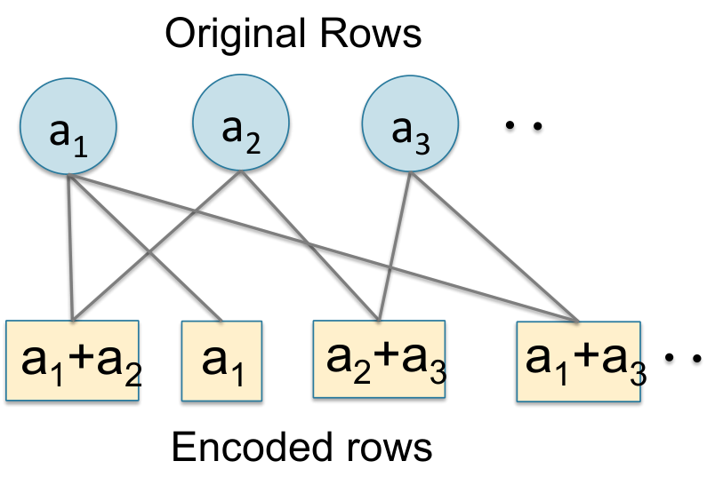
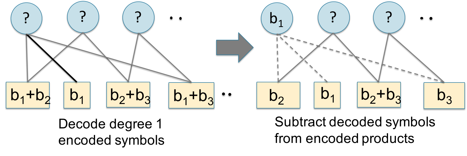
The rateless coded matrix-vector multiplication algorithm generates $m_{e}=\alpha m$ ($\alpha>1$) coded linear combinations of the $m$ rows of matrix $\mathbf{A}$ and distributes them equally across $p$ worker nodes. Each of these linear combinations is generated by choosing $d$ of the $m$ rows uniformly at random and adding them. For example, if $d=2$, and we choose rows $\mathbf{a}_{1}$ and $\mathbf{a}_{3}$ of $\mathbf{A}$, then the encoded row is $\mathbf{a}_{1}+\mathbf{a}_{3}$, as shown in Fig. 5a. The value $d$, referred to as the degree of the linear combination is an i.i.d. realization of a carefully chosen degree distribution $\rho(d)$. For LT codes, $\rho(d)$ is the Robust Soliton distribution (given in (4) below). Each worker receives $m_{e}/p$ encoded rows of matrix $\mathbf{A}$ and a copy of the vector $\mathbf{x}$. It computes row-vector products, for example $(\mathbf{a}_{1}+\mathbf{a}_{3})^{T}\mathbf{x}=b_{1}+b_{3}$ for the encoded row $(\mathbf{a}_{1}+\mathbf{a}_{3})$, and sends them back to the master node. Due to the carefully chosen degree distribution $\rho(d)$, the master node can use an iterative peeling decoder (Luby, 2002) (illustrated in Fig. 5b) to recover each element of the product vector $\mathbf{b}=\mathbf{A}\mathbf{x}$ with a low decoding complexity of $\mathcal{O}(\log m)$. Overall, it needs to wait for any $M^{\prime}=m(1+\epsilon)$ row-vector products to be completed across all the nodes, where $\epsilon$ is a small overhead; $\epsilon\rightarrow 0$ as $m\rightarrow\infty$).

To the best of our knowledge, our work is the first to exploit the rateless nature of LT codes to perform load-balancing in distributed matrix computations and utilize all the partial work done by slow workers. We also provide the first theoretical analysis of the latency achieved by this strategy with ideal load balancing and show that it asymptotically achieves near-perfect latency and computation cost. Previous works (Severinson et al., 2017; Wang et al., 2018) do not present such analyses. Moreover, we present extensive experimental results on $3$ different computing environments: local parallel computing, distributed computing on Amazon EC2 and serverless computing on Amazon Lambda.

Besides proposing the rateless coding strategy, one of the main contributions of our work is to theoretically analyze and compare it with ideal load balancing. In particular, we consider two performance metrics: 1) latency $T$, which is the time until $\mathbf{b}=\mathbf{A}\mathbf{x}$ can be recovered by the master, and 2) number of computations $C$, which is the number of row-vector product tasks completed by the $p$ workers until $\mathbf{b}$ can be recovered. We consider a simple delay model where worker $i$ has an initial delay of $X_{i}$ after which it spends a constant time $\tau$ per row-vector product task.

This results shows that as long as the number of encoded rows $m_{e}$ is sufficiently larger than $m$, despite not performing dynamic task assignment, the rateless coding strategy can seamlessly adapt to varying initial delays at the workers. Its runtime $T_{\text{LT}}$ and $C_{\text{LT}}$ asymptotically converge to the ideal strategy. The exact results are derived in Theorem 3 and Theorem 4.

The rest of the paper is organized as follows. Section 2 presents the system model, performance criteria and comparison benchmarks. Section 3 describes our rateless fountain coding strategy for distributed matrix-vector multiplication. Section 4 shows theoretical analyses and a latency-cost comparison of rateless coding with other strategies. Section 5 extends these results to the queueing setting where vectors $\mathbf{x}_{1},\mathbf{x}_{2},\ldots$ that need to be multiplied with matrix $\mathbf{A}$ arrive at rate $\lambda$. Experimental results are presented in Section 6. All proofs are deferred to the Appendix.

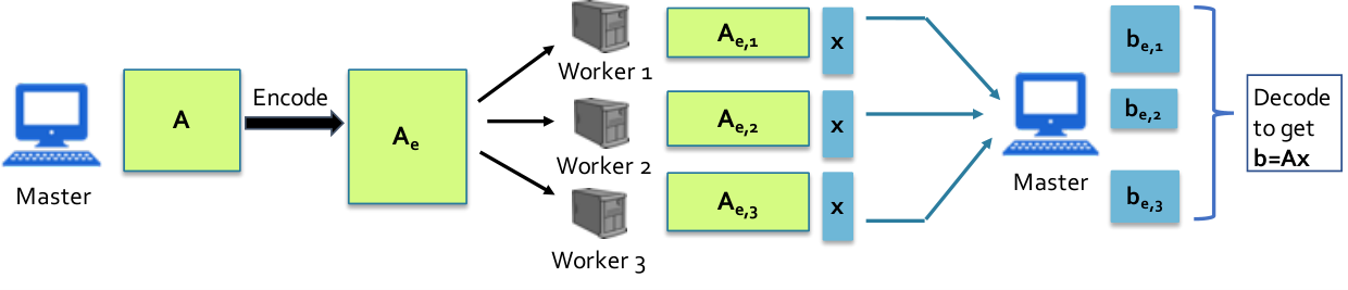
Consider the problem of multiplying a $m\times n$ matrix $\mathbf{A}$ with a $n\times 1$ vector $\mathbf{x}$ using $p$ worker nodes and a master node as shown in Fig. 3. The worker nodes can only communicate with the master, and cannot directly communicate with other workers. The goal is to compute the result $\mathbf{b}=\mathbf{A}\mathbf{x}$ in a distributed fashion and mitigate the effect of unpredictable node slowdown or straggling. The rows of $\mathbf{A}$ are encoded using an error correcting code to give the $m_{e}\times n$ encoded matrix $\mathbf{A_{e}}$, where $m_{e}\geq m$. We denote the amount of redundancy added by the parameter $\alpha=m_{e}/m$. Matrix $\mathbf{A_{e}}$ is split along its rows to give $p$ submatrices $\mathbf{A_{e}}_{,1},\ldots,\mathbf{A_{e}}_{,p}$ of equal size such that worker $i$ stores submatrix $\mathbf{A_{e}}_{,i}$. To compute the matrix-vector product $\mathbf{b}=\mathbf{A}\mathbf{x}$, the vector $\mathbf{x}$ is communicated to the workers such that Worker $i$ is tasked with computing the product $\mathbf{A_{e}}_{,i}\mathbf{x}$.

To complete the assigned task, each worker needs to compute a sequence of row vector products of the form $\mathbf{a}_{\mathbf{e},j}\mathbf{x}$ where $\mathbf{a}_{\mathbf{e},j}$ is the $j^{\text{th}}$ row of $\mathbf{A_{e}}$. The time taken by a worker node to finish computing one or more row-vector products may be random due to variability in the node speed or variability in the amount of computation assigned to it. The master node aggregates the computations of all, or a subset of, the workers into the vector $\mathbf{b_{e}}$, which is then decoded to give the final result $\mathbf{b}=\mathbf{A}\mathbf{x}$. If $\mathbf{b_{e}}$ is not decodable, the master waits until workers compute more row-vector products.

We use the following metrics to compare different distributed matrix-vector multiplication schemes via theoretical analysis and associated simulations (Section 4), and experiments in parallel, distributed, and serverless environments (Section 6).

For any strategy we always have $C\geq m$ where $m$ is the number of rows of $\mathbf{A}$ or the number of elements in $\mathbf{b}$.

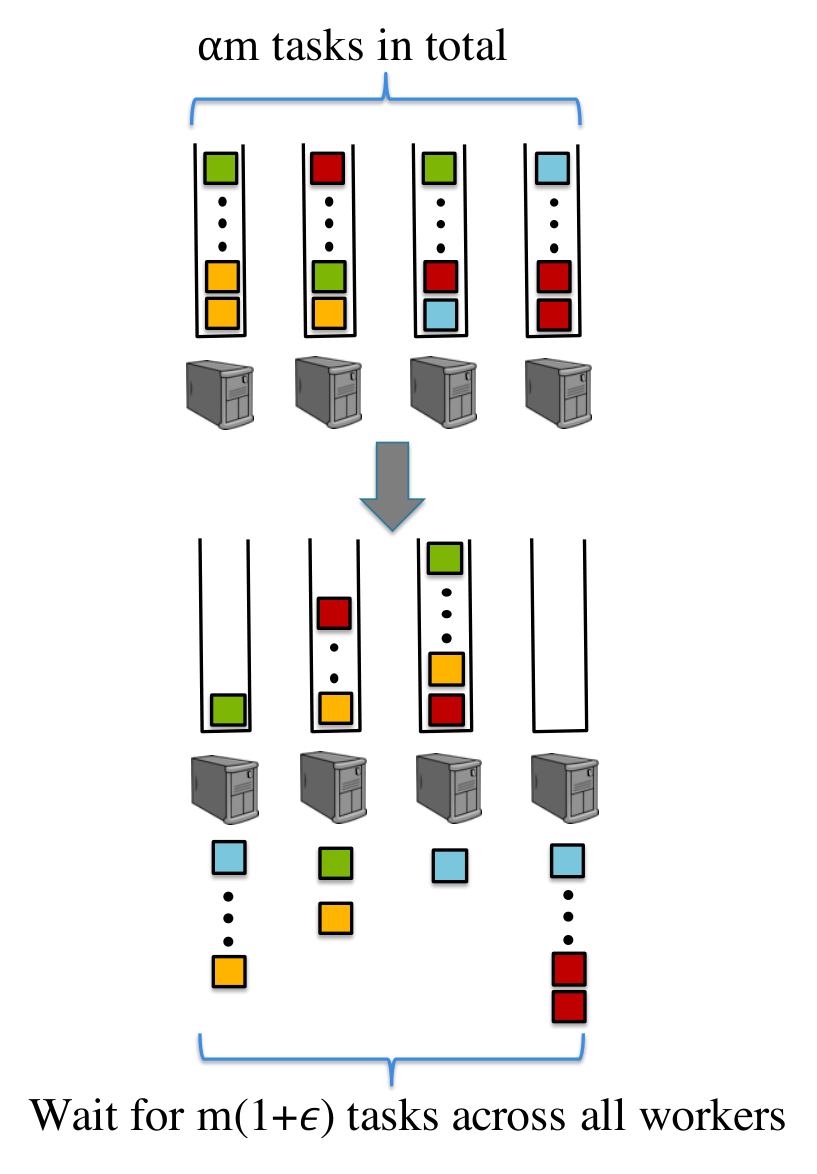
We compare the performance of the proposed rateless coded strategy with three benchmarks: ideal load balancing, $r$-replication, and the $(p,k)$ MDS-coded strategy, which are described formally below. Fig. 4 illustrates the differences in the way row-vector product tasks are assigned to and collected from workers in each strategy.

Ideal Load Balancing. The multiplication of the $m\times n$ matrix $\mathbf{A}$ with the $n\times 1$ vector $\mathbf{x}$ can be treated as a job with $m$ tasks, where each task corresponding to one row-vector product. In the ideal load balancing strategy, the master node maintains a central queue of these $m$ tasks. It dynamically assigns one task to each of the $p$ workers as soon as a worker finishes its previous task. The matrix-vector multiplication is complete when exactly $m$ tasks are collectively finished by the workers. This strategy seamlessly adapts to varying worker speeds without performing any redundant computation ($C=m$); hence it gives the optimal latency-computation trade-off. This strategy may be impractical due to the constant communication between the master and the worker nodes. Nevertheless, it serves as a good theoretical benchmark for comparison with the rateless, replication and MDS strategies.

The $r-$Replication Strategy. A simple distributed multiplication strategy is to split $\mathbf{A}$ along its rows into $p/r$ submatrices $\mathbf{A}_{1},\ldots,\mathbf{A}_{p/r}$, with $rm/p$ rows each (assume that $p/r$ divides $m$) and multiply each submatrix with $\mathbf{x}$ in parallel on $r$ distinct worker nodes. The master collects the results from the fastest of the $r$ nodes that have been assigned the task of computing the product $\mathbf{A}_{i}\mathbf{x}$ for all $i$. The computed products are aggregated into the $m\times 1$ vector $\mathbf{b}$. Setting $r=1$ corresponds to the naive or uncoded strategy where $\mathbf{A}$ is split into $p$ sub-matrices and each worker node computes the corresponding submatrix-vector product. While this approach performs the least number of computations it is susceptible to straggling nodes or node failures. Increasing the number of replicas provides greater straggler tolerance at the cost of redundant computations. Real distributed computing frameworks like MapReduce (Dean and Ghemawat, 2008) and Spark (Zaharia et al., 2010) often use $r=2$ i.e. each computation is assigned to $2$ different worker nodes for added reliability and straggler tolerance.

The $(p,k)$ MDS Coded Strategy. Recent works like (Lee et al., 2017a; Li et al., 2016) have applied MDS coding to overcome the problem of stragglers in the uncoded strategy. The strategy involves pre-multiplying $\mathbf{A}$ at the central node with a suitable encoding matrix $\mathbf{F}$ denoting the MDS codes. For encoding using a $(p,k)$ MDS code, the matrix $\mathbf{A}$ is split along its rows into $k$ matrices $\mathbf{A}_{1},\ldots,\mathbf{A}_{k}$, each having $m/k$ rows. The MDS code adds $p-k$ redundant matrices $\mathbf{A}_{k+1},\ldots,\mathbf{A}_{p}$ which are independent linear combinations of the matrices $\mathbf{A}_{1},\ldots,\mathbf{A}_{k}$. Worker $i$ computes the product $\mathbf{A}_{i}\mathbf{x}$. Thus the system is robust to $p-k$ stragglers. However this strategy adds a significant computation overhead. When none of the nodes are slow, the system performs $mp/k$ row-vector products (as opposed to $m$ row-vector products in the uncoded case).

Luby Transform (LT) codes proposed in (Luby, 2002) are a class of erasure codes that can be used to generate a limitless number of encoded symbols from a finite set of source symbols. We apply LT codes to matrix-vector multiplication by treating the $m$ rows of the matrix $\mathbf{A}$ as source symbols. Each encoded symbol is the sum of $d$ source symbols chosen uniformly at random from the matrix rows. Thus if $\mathcal{S}_{d}\subseteq\{1,2,\dots m\}$ is the set of $d$ row indices, the corresponding encoded row is $\mathbf{a}_{\mathbf{e}}=\sum_{i\in\mathcal{S}_{d}}\mathbf{a}_{i}$.

The number of original rows in each encoded row, or the degree $d$, is chosen according to the Robust Soliton degree distribution

where $R=c\log(m/\delta)\sqrt{m}$ for some $c>0$ and $\delta\in[0,1]$, with $c$ and $\delta$ being design parameters. Some guidelines for choosing $c$ and $\delta$ can be found in (MacKay, 2003). The probability of choosing $d=d_{0}$ is equal to $\rho(d_{0})/\sum_{i=1}^{m}\rho(i)$. Once the degree $d$ is chosen, encoding is performed by choosing $d$ source symbols uniformly at random (this determines $\mathcal{S}_{d}$) and adding them to generate an encoded symbol. The encoding process is illustrated in Fig. 5a.

Once the rows of the encoded matrix $\mathbf{A_{e}}$ are generated, we can compute the encoded matrix vector product $\mathbf{b_{e}}=\mathbf{A_{e}}\mathbf{x}$. To decode the desired matrix vector product $\mathbf{b}=\mathbf{A}\mathbf{x}$ from a subset of $M^{\prime}$ symbols of $\mathbf{b_{e}}$ we use the the iterative peeling decoder described in (Luby, 2002; Shokrollahi, 2006; Shokrollahi et al., 2011). If $\mathbf{b}=[b_{1},b_{2},\dots b_{m}]$, the decoder may receive symbols $b_{1}+b_{2}+b_{3}$, $b_{2}+b_{4}$, $b_{3}$, $b_{4}$, and so on since each row of $\mathbf{A_{e}}$ is a sum of some rows of $\mathbf{A}$. Decoding is performed in an iterative fashion. In each iteration, the decoder finds a degree one encoded symbol, covers the corresponding source symbol, and subtracts the symbol from all other encoded symbols connected to that source symbols. This decoding process is illustrated in Fig. 5b.

Since the encoding uses a random bipartite graph, the number of symbols required to decode the $m$ source symbols successfully is a random variable $M^{\prime}$ which we call the decoding threshold,

For the Robust Soliton distribution, (Luby, 2002) gives the following high probability bound on $M^{\prime}$.

The $m\times n$ matrix $\mathbf{A}$ is encoded to generate an $m_{e}\times n$ encoded matrix $\mathbf{A_{e}}$ where $m_{e}=\alpha m$. Each row of $\mathbf{A_{e}}$ is the sum of a random subset of rows of $\mathbf{A}$ as described in Section 3.1. The knowledge of the mapping between the rows of $\mathbf{A}$ and the rows of $\mathbf{A_{e}}$ is crucial for successful decoding as illustrated in Figures 5a and 5b. Hence this mapping is stored at the master. The encoding step can be treated as a pre-processing step in that it is only performed initially.

The $\alpha m$ rows of the encoded matrix are distributed equally among the $p$ worker nodes as illustrated in Fig. 3. To multiply $\mathbf{A}$ with a vector $\mathbf{x}$, the master communicates $\mathbf{x}$ to the workers. Each worker multiplies $\mathbf{x}$ with each row of $\mathbf{A_{e}}$ stored in its memory and returns the product (a scalar) to the master. The master collects row-vector products of the form $\textbf{a}_{\textbf{e},j}\mathbf{x}$ (elements of $\mathbf{b_{e}}$) from the workers until it has enough elements to be able to recover $\mathbf{b}$. If a worker node completes all the $\alpha m/p$ row-vector products assigned to it before the master is able to decode $\mathbf{b}$, it will remain idle, while the master collects more row-vector products from other workers.

Once the master has collected a sufficient number of coded row-vector products from the workers it can recover the desired matrix vector product $\mathbf{b}=\mathbf{A}\mathbf{x}$ from the subset of the elements of $\mathbf{b_{e}}=\mathbf{A_{e}}\mathbf{x}$ that it has collected using the iterative peeling decoder. Once the master decodes all elements of the product vector $\mathbf{b}=\mathbf{A}\mathbf{x}$, it sends a done signal to all workers nodes to stop their local computation.

The following modifications can make the current implementation even more efficient in real systems:

1. (1)

   Blockwise Communication: To truly monitor the partial work done by each worker the master needs to receive each encoded row-vector product $\mathbf{a}_{\mathbf{e},j}\mathbf{x}$ from the workers. However this imposes a large communication overhead which may increase latency in a slow network. To prevent this, in our distributed computing experiments, we communicate submatrix-vector products $\mathbf{A_{e}}_{i}^{j}\mathbf{x}$ where $\mathbf{A_{e}}_{i}^{j}$ is the $j^{\text{th}}$ part of the encoded submatrix $\mathbf{A_{e}}_{i}$ stored at worker $i$, and each part corresponds to approximately $10\%$ of the total rows of the submatrix. Note that if $\mathbf{A}$ is very large then it will not be feasible for worker $i$ to read the entire submatrix $\mathbf{A_{e}}_{i}$ from memory at once. As a result $\mathbf{A_{e}}_{i}\mathbf{x}$ needs to be computed in parts for any coding scheme.

2. (2)

   Using Raptor Codes: Despite their ease of implementation and fast decoding, LT codes (Luby, 2002) are sub-optimal in practice due to the overhead of $M^{\prime}-m$ extra symbols required to decode the original $m$ source symbols. In our experiments we observe that for a matrix $\mathbf{A}$ with $m=11760$ rows, we need to wait for $12500$ encoded row-vector products to decode $\mathbf{b}=\mathbf{A}\mathbf{x}$ with $99\%$ probability. Advanced rateless codes like Raptor Codes (Shokrollahi, 2006) can decode $m$ source symbols from $m(1+\epsilon)$ symbols for any constant $\epsilon$ even for finite values of $m$. Since Raptor Codes are the rateless codes used in practical wireless standards (Shokrollahi et al., 2011) we expect them to be used in practical implementations of our coded distributed matrix vector multiplication strategy to improve efficiency.

3. (3)

   Using Systematic Rateless Codes: We can entirely avoid decoding (in the absence of significant straggling) by using Systematic LT/Raptor Codes (Shokrollahi, 2006) where the $m$ source rows $\mathbf{a}_{1},\mathbf{a}_{2},\dots\mathbf{a}_{m}$ form a subset of the encoded rows in $\mathbf{A_{e}}$. The overall scheme can be designed so that each worker first computes the row-vector products corresponding to the systematic symbols $\mathbf{a}_{1},\mathbf{a}_{2},\dots\mathbf{a}_{m}$ and then computes other encoded products (in the event of node slowdown). This would preclude the need for decoding if there is no/little straggling thereby reducing the overall latency.

We assume that worker $i$ requires time $Y_{i}$ to perform $B_{i}$ row-vector product computations where

Thus, the delay involves the sum of two components: 1) a random variable $X_{i}$ that includes initial setup time at the worker before it actually begins performing the computations, and 2) a shift that is linear in the number of computations performed at the worker. This delay model is motivated by the observations of (Dean and Barroso, 2013) where it is noted that the variability in latency arises largely from delays due to background tasks running at worker nodes and that once a request actually begins execution, the variability is considerably lower. When $X_{i}$ is exponentially distributed with rate $\mu$, the time taken by worker $i$ to perform $b$ computations is distributed as

While this follows the shifted exponential delay models used in (Lee et al., 2017a), (Dutta et al., 2016) and (Dutta et al., 2017), the key difference is that the shift is parameterized by the number of computations at each worker. We believe this is a more realistic model as it captures the effect of increasing the amount of computations on the delay – if a worker is assigned more computations, there is larger delay. Moreover, unlike previous works, the decay rate $\mu$ of the exponential part of the delay does not change with the number of computations performed by that worker. Fig. 6 illustrates our delay model.

Also, in our analysis, we use $X_{k:p}$ to denote the $k^{\text{th}}$ order statistic i.e. the $k^{\text{th}}$ smallest of $p$ random variables $X_{1},\ldots,X_{p}$ and we define $U_{l}=X_{l+1:p}-X_{l:p}$, $l=1,\ldots,p-1$ as the difference of consecutive order statistics. We also use the notation $H_{j}=\sum_{v=1}^{j}1/v$, for the $j^{\text{th}}$ Harmonic number.

Recall that in the ideal load balancing strategy, we have a central queue at the master and tasks being allocated to a worker as soon as it becomes idle (either immediately after the initial delay or after it completes the current task) as illustrated in Fig. 6. Thus it computes exactly $C=m$ row-vector products in total when an $m\times n$ matrix is multiplied with $n\times 1$ vector and performs zero redundant computations. Theorem 2 below proves the optimality of ideal load balancing in terms of latency and Lemma 2 and Corollary 1 give bounds on the expected latency.

Note that the ideal load balancing scheme is not exactly realizable in practice. Approaches like work stealing (Dinan et al., 2007; Harlap et al., 2016) can potentially approximate this strategy by physically moving tasks from busy workers to idle workers. However implementing such approaches may not be feasible in all settings, for e.g. when the communication latency between workers is too large, or the data is restricted to lie on a particular worker due to privacy concerns. In this work we aim to show that it is possible to algorithmically achieve near-ideal latency performance for matrix-vector multiplication by using the rateless coded computing strategy described in Section 3 which does not require physically moving data between workers.

We make the following assumption for analyzing the latency of the proposed rateless coded strategy.

We believe the above assumption is reasonable because the problem of distributed matrix vector multiplication arises only when $m$ (the number of rows of $\mathbf{A}$) is large and the high probability bound of Lemma 1 can be used to show that $\mathbb{E}[M^{\prime}]=m(1+\epsilon)$, where $\epsilon\rightarrow 0$ as $m\rightarrow\infty$. Note that this assumption is only to facilitate a better theoretical comparison between the LT coded and ideal strategies. In our experiments in Section 6 we choose a value of $M^{\prime}$ according to Lemma 1 that is slightly larger than $m$ and ensures that the original matrix-vector product $\mathbf{b}=\mathbf{A}\mathbf{x}$ can be recovered with high $(>99\%)$ probability.

However in practice, we cannot set $\alpha=m_{e}/m\rightarrow\infty$ owing to limitations in computation power and memory at workers. Instead the amount of redundancy in the LT coded strategy is fixed initially by choosing the number of encoded rows $m_{e}=\alpha m/p$ for some $\alpha>1$. Computations are divided equally among the $p$ workers and thus each worker can perform a maximum of $\alpha m/p$ computations.

Thus as $\alpha$ (and consequently $m_{e}$) increases, $T_{\text{LT}}$ is equal to $T_{\text{ideal}}$ with a high probability. A cleaner result is obtained for the case when $X_{i}\sim\exp(\mu)$, as given below.

We also derive an upper bound on the difference between the expected latencies of the rateless and the ideal strategies. We only state the result for $X_{i}\sim\exp(\mu)$ over here and defer the (more complicated) general result and its proof to Appendix C.

The second term decays exponentially and dominates the first term, which is a polynomial. The rate of decay increases as the amount of redundancy $\alpha$ increases. In other words, $\mathbb{E}[T_{\text{LT}}]$ approaches $\mathbb{E}[T_{\text{ideal}}]$ exponentially fast as redundancy is increased.

In the following subsections (and in Appendix E) we show that the latency of the MDS and Replication strategies is much larger than that of ideal load balancing and does not converge to $T_{\text{ideal}}$ on increasing redundancy. We also show that the number of computations performed by both replication and MDS coding in computing $\mathbf{b}=\mathbf{A}\mathbf{x}$ is much larger than $m$.

Recall that for the $(p,k)$ MDS coded strategy, the encoded submatrices $\mathbf{A_{e}}_{1}$,$\ldots$,$\mathbf{A_{e}}_{p}$ are generated by applying a $(p,k)$ MDS Code to submatrices $\mathbf{A}_{1},\ldots,\mathbf{A}_{k}$. The master then waits for the fastest $k$ workers to complete all the tasks assigned to them.

Observe that in (14) above, adding redundancy (reducing $k$) leads to an increase in the first term (more computation at each node) and decrease in the second term (less delay due to stragglers). Thus, straggler mitigation comes at the cost of additional computation at the workers which might even lead to an increase in latency. This is in contrast to Theorems 3 and 4 which indicates that the expected latency of the rateless coded strategy always decreases on adding redundancy (increasing $\alpha$). Moreover, the presence of the log-factor in the second term causes $T_{\text{MDS}}$ to always be larger than $T_{\text{ideal}}$ since there is no log-factor in the term containing $1/\mu$ in the upper bound on $T_{\text{ideal}}$ (Lemma 2).

We now analyze the number of computations performed by the $(p,k)$ MDS coding. The following result shows that with a high probability, the number of computations performed by the MDS Coded strategy is very close to the worst-case number of computations ($mp/k$) i.e. when all the workers perform all the tasks assigned to them in time $T_{\text{MDS}}$.

Even for a small value of $C_{0}$ in the above expression, $\Pr(C_{\text{MDS}}\geq\frac{mp}{k}-C_{0})$ can be very large. Thus the overhead $C_{\text{MDS}}-m$ is quite large (we only need $m$ computations in the uncoded case to reconstruct the $m$-dimensional matrix-vector product).

The $r-Replication$ strategy involves replicating each of the $p/r$ submatrices $\mathbf{A}_{1},\ldots,\mathbf{A}_{p/r}$ at $r$ distinct workers and selecting the result of the fastest worker for each submatrix.

Once again we see that adding redundancy (increasing $r$) leads to an increase in the first term (more computation at each node) and decrease in the second term (less delay due to stragglers). Thus the extra computation at the workers may lead to an increase in latency even in this case. Moreover the log-factor in the second term causes $T_{\text{Rep}}$ to always be larger than $T_{\text{ideal}}$, just like $T_{\text{MDS}}$.

Thus with a high probability, the number of computations performed is very close to the worst-case number ($mr$) i.e. when all the workers perform all the tasks assigned to them in time $T_{\text{rep}}$.

We simulate the MDS, replication, and LT-coded schemes under our delay model 5 for distributed matrix-vector multiplication with $m=10000$ matrix rows, $p=10$ workers and delay model parameters $\mu=1.0,\tau=0.001$ (Fig. 7). We limit the amount of redundancy to $\alpha=m_{e}/m\leq 2.0$ since this is the amount of redundancy in the basic $2$-replication scheme. Observe that the LT coded strategy ($\alpha=2.0$) clearly outperforms MDS coding (with $k=8$) in that it not only exhibits near-ideal latency (Fig. 7a) but also performs fewer total computations (Fig. 7b) than MDS coding. Changing $k$ does not improve the performance of MDS coding much. Specifically, increasing redundancy (reducing $k$) in MDS coding leads to higher latency after a point, as illustrated in Fig. 1 (and as expected from Lemma 3). On the other hand, the latency of LT coding converges to that of the Ideal scheme on increasing $\alpha$, without any increase in computations. Additional simulations for $X_{i}\sim\text{Pareto}(1,3)$ given in Fig. 11 in Appendix F also show similar improvements with LT coding.

We consider multiplication of a $10000\times 10000$ matrix $\mathbf{A}$ of random integers with a $10000\times 1$ vector $\mathbf{x}$ of random integers on an iMac Desktop with 8 GB of RAM and a 3.6 GHz Intel i7 Processor. This computation is parallelized over 100 processes using Python’s Multiprocessing Library (Foundation, [n. d.]). We compare the uncoded, 2-replication, MDS coding ($k=80,50$) and LT coding ($\alpha=1.25,2.0$) approaches. For fair comparison, we consider instances of MDS and LT codes that have the same number of encoded rows $m_{e}$. The encoded matrix $\mathbf{A_{e}}$ was divided equally among the $p=100$ processes and the experiment was repeated $10$ times with a different random $\mathbf{x}$ each time. The processes multiply the rows of $\mathbf{A_{e}}$ with $\mathbf{x}$ in parallel and we record the average latency (time required to collect enough row-vector products for successful decoding) and total computations. Results of average latency (Fig. 8a) show that LT coded and MDS coded approaches are clearly faster (about at least $1.2\times-$) than the Uncoded and 2-Replication approaches while Fig. 8d shows that the LT coded approaches also perform fewer total computations than the MDS or 2-replication strategies thus leading to more efficient resource utilization. Note that while MDS coding with $k=80$ has latency comparable to that of LT coding (both for $\alpha=1.25$ and $\alpha=2.0$), both latency and total computations with MDS coding increase on increasing $k$ to $50$ due to the higher computational load at each node (as discussed in Section 4). Recall that $k$ corresponds to the number of "fast" workers in the system. In most real systems the number of "fast" workers is transient and thus, unpredictable. Our experiments show that MDS coding is highly sensitive to the choice of $k$ with incorrect choices leading to higher latency. LT Coding on the other hand is not only fast, but is also insensitive to the amount of redundancy ($\alpha$) in that, the system designer can choose $\alpha$ to be as large as permitted by memory constraints without a risk of loss in performance (unlike MDS).

We created a cluster of 70 t2.small workers on AWS EC2 (Amazon, 2006) using Kubernetes (Google, 2015). Each worker was allocated 1 GB of memory. Computations were performed using Dask (Dask Development Team, 2016), a popular framwork for parallel computing in Python. A $11760\times 9216$ matrix $\mathbf{A}$ was extracted from the STL-10 (Coates et al., 2011) dataset. Once again we compared the uncoded, 2-replication, MDS coding ($k=56,35$) and LT coding ($\alpha=1.25,2.0$) approaches. The encoded matrix $\mathbf{A_{e}}$ is divided equally among the $p=70$ workers and multiplied with 5 different vectors, each of length $9216$, also extracted from the STL-10 (Coates et al., 2011) dataset. Fig. 8b shows the average latency of the different approaches. Both LT coded approaches are almost $2\times-$ faster than the MDS coded appraoches in this setting and almost $3\times-$ faster than the uncoded approaches. Each worker computes approximately $14$ row-vector products at a time before communicating the results to the master. This corresponds to approximately $10\%$ of the data stored in the workers memory thus balancing excessive communication (if results were communicated after every row-vector product computation) and memory limitations (if submatrices at the workers are too large to be communicated as a single chunk). Fig. 8e shows that the LT coded strategies also perform fewer total computations than MDS or $2$-replication. Additional experiments in Appendix F show that LT coding also demonstrates greater resilience to node failures than Replication or MDS coding in this setting.

We also performed experiments in the serverless computing environment AWS Lambda (Amazon, 2014). Serverless computing eschews the master-worker set-up in favor of only workers (resources) which read data from storage, perform computations on the data, and write it back to storage. Any further computations (like decoding) can be performed as and when desired by re-reading data from storage. As described in (Gupta et al., 2018), there is typically significant variability (straggling) across workers in this setting and therefore we expect to obtain speedups through coding. We use Numpywren (Shankar et al., 2018) for performing linear algebra on AWS Lambda. We multiply a $100000\times 10000$ matrix $\mathbf{A}$ (approximately $10\times-$ larger than $\mathbf{A}$ in the previous two experiments) with a $10000\times 1$ vector $\mathbf{x}$ in this setting. We compare the uncoded, MDS-Coded ($k=80$) and LT-coded ($\alpha=2.0$) approaches. As per the requirements of (Shankar et al., 2018), the encoding is performed over blocks of $10$ rows instead of individual rows. Our results, averaged over 5 trials, are presented in Figures 8c and 8f. They clearly show that the LT coded approach is faster than previous approaches, and performs fewer computations than MDS coding. We note that the experimental nature of current serverless computing frameworks makes it challenging to perform fine-grained logging of task times and to use larger encoded matrices (larger $\alpha$). Thus we expect even better results once the limitations of current frameworks have been resolved.

References

- Amazon (2006) Amazon. 2006. Amazon Web Services EC2. https://aws.amazon.com/ec2/.
- Amazon (2014) Amazon. 2014. Amazon Web Services Lambda. https://aws.amazon.com/lambda/.
- Ames (2014) William F Ames. 2014. Numerical Methods for Partial Differential Equations. Academic Press.
- Ananthanarayanan et al. (2013) Ganesh Ananthanarayanan, Ali Ghodsi, Scott Shenker, and Ion Stoica. 2013. Effective Straggler Mitigation: Attack of the Clones.. In USENIX Symposium on Networked Systems Design and Implementation (NSDI), Vol. 13. 185–198.
- Ananthanarayanan et al. (2010) Ganesh Ananthanarayanan, Srikanth Kandula, Albert G Greenberg, Ion Stoica, Yi Lu, Bikas Saha, and Edward Harris. 2010. Reining in the Outliers in Map-Reduce Clusters using Mantri.. In USENIX Symposium on Operating Systems Design and Implementation (OSDI), Vol. 10. 24.
- Coates et al. (2011) Adam Coates, Andrew Ng, and Honglak Lee. 2011. An analysis of single-layer networks in unsupervised feature learning. In Proceedings of the fourteenth international conference on artificial intelligence and statistics. 215–223.
- Dally (2015) William Dally. 2015. High-performance Hardware for Machine Learning. NIPS Tutorial (2015).
- Dask Development Team (2016) Dask Development Team. 2016. Dask: Library for dynamic task scheduling. https://dask.org
- David and Nagaraja (2003) H. A. David and H. N. Nagaraja. 2003. Order statistics. John Wiley, Hoboken, N.J.
- Dean and Barroso (2013) Jeffrey Dean and Luiz André Barroso. 2013. The tail at scale. Commun. ACM 56, 2 (2013), 74–80.
- Dean and Ghemawat (2008) Jeffrey Dean and Sanjay Ghemawat. 2008. MapReduce: simplified data processing on large clusters. Commun. ACM 51, 1 (2008), 107–113.
- Dinan et al. (2009) James Dinan, D Brian Larkins, Ponnuswamy Sadayappan, Sriram Krishnamoorthy, and Jarek Nieplocha. 2009. Scalable work stealing. In High Performance Computing Networking, Storage and Analysis, Proceedings of the Conference on. IEEE, 1–11.
- Dinan et al. (2007) James Dinan, Stephen Olivier, Gerald Sabin, Jan Prins, P Sadayappan, and Chau-Wen Tseng. 2007. Dynamic load balancing of unbalanced computations using message passing. In Parallel and Distributed Processing Symposium, 2007. IPDPS 2007. IEEE International. IEEE, 1–8.
- Dutta et al. (2016) Sanghamitra Dutta, Viveck Cadambe, and Pulkit Grover. 2016. Short-dot: Computing large linear transforms distributedly using coded short dot products. In Advances In Neural Information Processing Systems. 2100–2108.
- Dutta et al. (2017) Sanghamitra Dutta, Viveck Cadambe, and Pulkit Grover. 2017. Coded convolution for parallel and distributed computing within a deadline. In IEEE International Symposium on Information Theory (ISIT). IEEE, 2403–2407.
- Dutta et al. (2018) Sanghamitra Dutta, Mohammad Fahim, Farzin Haddadpour, Haewon Jeong, Viveck Cadambe, and Pulkit Grover. 2018. On the Optimal Recovery Threshold of Coded Matrix Multiplication. arXiv preprint arXiv:1801.10292 (2018).
- Foundation ([n. d.]) Python Software Foundation. [n. d.]. Multiprocessing. https://docs.python.org/3/library/multiprocessing.html.
- Fox et al. (1987) Geoffrey C. Fox, Steve W. Otto, and Anthony JG. Hey. 1987. Matrix Algorithms on a Hypercube I: Matrix Multiplication. Parallel Comput. 4, 1 (1987), 17–31.
- Gardner et al. (2016) K. Gardner, M. Harchol-Balter, and A. Scheller-Wolf. 2016. A Better Model for Job Redundancy: Decoupling Server Slowdown and Job Size. In Proceedings of IEEE MASCOTS.
- Gardner et al. (2015a) K. Gardner, S. Zbarsky, S. Doroudi, M. Harchol-Balter, E. Hyytiä, and A. Scheller-Wolf. 2015a. Reducing Latency via Redundant Requests: Exact Analysis. In Proceedings of the ACM SIGMETRICS.
- Gardner et al. (2015b) K. Gardner, S. Zbarsky, M. Harchol-Balter, and A. Scheller-Wolf. 2015b. Analyzing Response Time in the Redundancy-d System. In CMU-CS-15-141 archive.
- Google (2015) Google. 2015. Kubernetes. https://kubernetes.io.
- Gupta et al. (2018) Vipul Gupta, Shusen Wang, Thomas Courtade, and Kannan Ramchandran. 2018. Oversketch: Approximate matrix multiplication for the cloud. In 2018 IEEE International Conference on Big Data (Big Data). IEEE, 298–304.
- Halbawi et al. (2017) Wael Halbawi, Navid Azizan-Ruhi, Fariborz Salehi, and Babak Hassibi. 2017. Improving distributed gradient descent using reed-solomon codes. arXiv preprint arXiv:1706.05436 (2017).
- Harchol-Balter (2013) Mor Harchol-Balter. 2013. Performance modeling and design of computer systems: queueing theory in action. Cambridge University Press.
- Harlap et al. (2016) Aaron Harlap, Henggang Cui, Wei Dai, Jinliang Wei, Gregory R Ganger, Phillip B Gibbons, Garth A Gibson, and Eric P Xing. 2016. Addressing the straggler problem for iterative convergent parallel ML. In Proceedings of the Seventh ACM Symposium on Cloud Computing. ACM, 98–111.
- Huang et al. (1984) Kuang-Hua Huang et al. 1984. Algorithm-based Fault Tolerance for Matrix Operations. IEEE Trans. Comput. 100, 6 (1984), 518–528.
- Huang et al. (2012) Longbo Huang, S. Pawar, Hao Zhang, and K. Ramchandran. 2012. Codes can reduce queueing delay in data centers. In IEEE International Symposium on Information Theory Proceedings (ISIT). 2766–2770.
- Joshi (2017) Gauri Joshi. 2017. Boosting Service Capacity via Adaptive Task Replication. SIGMETRICS Perform. Eval. Rev. 45, 2 (Oct. 2017), 9–11. https://doi.org/10.1145/3152042.3152046
- Joshi (2018) Gauri Joshi. 2018. Synergy via Redundancy: Boosting Service Capacity with Adaptive Replication. SIGMETRICS Performance Evaluation Review 45, 3 (March 2018), 21–28. http://doi.acm.org/10.1145/3199524.3199530
- Joshi et al. (2012) Gauri Joshi, Yanpei Liu, and Emina Soljanin. 2012. Coding for fast content download. In Allerton Conference on Communication, Control, and Computing. IEEE, 326–333.
- Joshi et al. (2014) Gauri Joshi, Yanpei Liu, and Emina Soljanin. 2014. On the Delay-Storage Trade-Off in Content Download from Coded Distributed Storage Systems. IEEE Journal on Selected Areas of Communications 32, 5 (May 2014), 989–997.
- Joshi et al. (2010) Gauri Joshi, Joong Bum Rhim, John Sun, and Da Wang. 2010. Fountain codes. In Global telecommunications conference (GLOBECOM 2010). 7–12.
- Joshi et al. (2015) Gauri Joshi, Emina Soljanin, and Gregory Wornell. 2015. Queues with redundancy: Latency-cost analysis. ACM SIGMETRICS Performance Evaluation Review 43, 2 (2015), 54–56.
- Joshi et al. (2017) Gauri Joshi, Emina Soljanin, and Gregory Wornell. 2017. Efficient Redundancy Techniques for Latency Reduction in Cloud Systems. ACM Transactions on Modeling and Performance Evaluation of Computing Systems 2, 12 (may 2017).
- Karakus et al. (2017) Can Karakus, Yifan Sun, and Suhas Diggavi. 2017. Encoded distributed optimization. In IEEE International Symposium on Information Theory (ISIT). IEEE, 2890–2894.
- Kim and Agrawala (1989) C. Kim and A. K. Agrawala. 1989. Analysis of the Fork-Join Queue. IEEE Trans. Comput. 38, 2 (Feb. 1989), 250–255.
- Kosaian et al. (2018) Jack Kosaian, K. V. Rashmi, and Shivaram Venkataraman. 2018. Learning a Code: Machine Learning for Approximate Non-Linear Coded Computation. CoRR abs/1806.01259 (2018). arXiv:1806.01259 http://arxiv.org/abs/1806.01259
- Kosaian et al. (2019) Jack Kosaian, K. V. Rashmi, and Shivaram Venkataraman. 2019. Parity Models: A General Framework for Coding-Based Resilience in ML Inference. CoRR abs/1905.00863 (2019). arXiv:1905.00863 http://arxiv.org/abs/1905.00863
- Kumar et al. (1994) Vipin Kumar, Ananth Grama, Anshul Gupta, and George Karypis. 1994. Introduction to Parallel Computing: Design and Analysis of Algorithms. Vol. 400. Benjamin/Cummings Redwood City.
- Lee et al. (2017a) Kangwook Lee, Maximilian Lam, Ramtin Pedarsani, Dimitris Papailiopoulos, and Kannan Ramchandran. 2017a. Speeding Up Distributed Machine Learning Using Codes. IEEE Transactions on Information Theory (2017).
- Lee et al. (2017b) Kangwook Lee, Nihar B. Shah, Longbo Huang, and Kannan Ramchandran. 2017b. The MDS Queue: Analysing the Latency Performance of Erasure Codes. IEEE Transactions on Information Theory 63, 5 (May 2017), 2822–2842.
- Li et al. (2017) Songze Li, Seyed Mohammadreza Mousavi Kalan, A Salman Avestimehr, and Mahdi Soltanolkotabi. 2017. Near-Optimal Straggler Mitigation for Distributed Gradient Methods. arXiv preprint arXiv:1710.09990 (2017).
- Li et al. (2016) Songze Li, Mohammad Ali Maddah-Ali, and A Salman Avestimehr. 2016. A Unified Coding Framework for Distributed Computing with Straggling Servers. In IEEE Global Communications Conference (GLOBECOM) Workshops. IEEE, 1–6.
- Luby (2002) Michael Luby. 2002. LT codes. In null. IEEE, 271.
- MacKay (2003) David JC MacKay. 2003. Information theory, inference and learning algorithms. Cambridge university press.
- Nelson and Tantawi (1988) R. Nelson and A. Tantawi. 1988. Approximate Analysis of Fork/Join Synchronization in Parallel Queues. IEEE Trans. Comput. 37, 6 (Jun. 1988), 739–743.
- Page et al. (1999) Lawrence Page, Sergey Brin, Rajeev Motwani, and Terry Winograd. 1999. The PageRank Citation Ranking: Bringing order to the Web. Technical Report. Stanford InfoLab.
- Severinson et al. (2017) Albin Severinson, Alexandre Graell i Amat, and Eirik Rosnes. 2017. Block-Diagonal and LT Codes for Distributed Computing With Straggling Servers. arXiv preprint arXiv:1712.08230 (dec 2017).
- Shah et al. (2016) Nihar B. Shah, Kangwook Lee, and Kannan Ramchandran. 2016. When Do Redundant Requests Reduce Latency? IEEE Transactions on Communications 64, 2 (Feb 2016), 715–722.
- Shankar et al. (2018) Vaishaal Shankar, Karl Krauth, Qifan Pu, Eric Jonas, Shivaram Venkataraman, Ion Stoica, Benjamin Recht, and Jonathan Ragan-Kelley. 2018. numpywren: serverless linear algebra. arXiv preprint arXiv:1810.09679 (2018).
- Shokrollahi (2006) Amin Shokrollahi. 2006. Raptor codes. IEEE/ACM Transactions on Networking (TON) 14, SI (2006), 2551–2567.
- Shokrollahi et al. (2011) Amin Shokrollahi, Michael Luby, et al. 2011. Raptor codes. Foundations and trends® in communications and information theory 6, 3–4 (2011), 213–322.
- Sun et al. (2016) Yin Sun, Can Emre Koksal, and Ness B. Shroff. 2016. On Delay-Optimal Scheduling in Queueing Systems with Replications. arXiv:1603.07322 (March 2016).
- Sun et al. (2015) Yin Sun, Zizhan Zheng, Can Emre Koksal, Kyu-Han Kim, and Ness B. Shroff. 2015. Provably Delay Efficient Data Retrieving in Storage Clouds. In Proceedings of the IEEE Conference on Computer Communications (INFOCOM).
- Tandon et al. (2017) Rashish Tandon, Qi Lei, Alexandros G Dimakis, and Nikos Karampatziakis. 2017. Gradient Coding: Avoiding Stragglers in Synchronous Gradient Descent. stat 1050 (2017), 8.
- Varki et al. (2008) Elizabeth Varki, Arif Merchant, and Hui Chen. 2008. The M/M/1 fork-join queue with variable sub-tasks. unpublished, available online (2008).
- Wang et al. (2014) Da Wang, Gauri Joshi, and Gregory Wornell. 2014. Efficient Task Replication for Fast Response times in Parallel Computation. In ACM SIGMETRICS Performance Evaluation Review, Vol. 42. ACM, 599–600.
- Wang et al. (2015) Da Wang, Gauri Joshi, and Gregory Wornell. 2015. Using Straggler Replication to Reduce Latency in Large-scale Parallel Computing. ACM SIGMETRICS Performance Evaluation Review 43, 3 (2015), 7–11.
- Wang et al. (2019) Da Wang, Gauri Joshi, and Gregory W. Wornell. 2019. Efficient Straggler Replication in Large-Scale Parallel Computing. ACM Trans. Model. Perform. Eval. Comput. Syst. 4, 2, Article 7 (April 2019), 23 pages. http://doi.acm.org/10.1145/3310336
- Wang et al. (2018) Sinong Wang, Jiashang Liu, and Ness Shroff. 2018. Coded Sparse Matrix Multiplication. arXiv preprint arXiv:1802.03430 (2018).
- Yang et al. (2017) Yaoqing Yang, Pulkit Grover, and Soummya Kar. 2017. Coded Distributed Computing for Inverse Problems. In Advances in Neural Information Processing Systems. 709–719.
- Yu et al. (2017a) Qian Yu, Mohammad Maddah-Ali, and Salman Avestimehr. 2017a. Polynomial codes: an optimal design for high-dimensional coded matrix multiplication. In Advances in Neural Information Processing Systems. 4406–4416.
- Yu et al. (2017b) Qian Yu, Mohammad Ali Maddah-Ali, and A Salman Avestimehr. 2017b. Coded Fourier Transform. arXiv preprint arXiv:1710.06471 (2017).
- Zaharia et al. (2010) Matei Zaharia, Mosharaf Chowdhury, Michael J Franklin, Scott Shenker, and Ion Stoica. 2010. Spark: Cluster computing with working sets. HotCloud 10, 10-10 (2010), 95.
Appendix A Properties of LT Codes
Fig. 9 shows simulation results for the number of symbols decoded successfully for each encoded symbol received. For this we perform LT-Coded multiplication of a randomly generated matrix with a vector. The matrix is encoded using an LT code with parameters and chosen according to the guidelines of (MacKay, 2003). We generate a single row of the encoded matrix at a time which is then multiplied with the size vector to give a single element of the encoded matrix vector product . The process is repeated until we have enough symbols for successfully decoding the entire size vector using the peeling decoder. The plots of Fig. 9 correspond to different choices of and . In each case we observe an avalanche behavior wherein very few symbols are decoded up to a point ( approximately up to encoded symbols received) after which the decoding proceeds very rapidly to completion. This effectively illustrates the fact that the computation overhead of the proposed LT coded matrix vector multiplication strategy is very small (). The theoretical encoding and decoding properties of LT codes are summarized in the following lemmas:
Lemma 7 (Theorem 13 in (Luby, 2002)).
For any constant , the average degree of an encoded symbol is where is the number of source symbols.
Corollary 5.
Each encoding symbol can be generated using symbol operations on average.
Lemma 8 (Theorem 17 in (Luby, 2002)).
For any constant and for a source block with source symbols, the LT decoder can recover all the source symbols from a set of with probability at least .
Corollary 6.
The expected decoding threshold is given by where as
Corollary 7.
Since the average degree of an encoded symbol is the decoding requires symbol operations on average.
Appendix B On the Order Statistics of Exponential Random Variables
We first state some standard results (David and Nagaraja, 2003) on order statistics of exponential random variables to aid the understanding of the latency analysis presented subsequently. If , , … are exponential random variables with rate , their order statistic is denoted by . Thus, , and . The expected value of is given by