Higgs mode in $2+1$ dimensional $O(2)$ model

Ji-Chong Yang Affiliation: Department of Physics & State Key Laboratory of Surface Physics, Fudan University,
Shanghai 200433, China Affiliation: Department of Physics, Liaoning Normal University, Dalian 116029, China Yu Shi Email: yushi@fudan.edu.cn Thanks: Corresponding author Affiliation: Department of Physics & State Key Laboratory of Surface Physics, Fudan University,
Shanghai 200433, China

August 24, 2026

Abstract

We investigate the spectral functions of the Higgs mode in $O(2)$ model, which can be experimentally realized in a 2D Bose gas. Zero temperature limit is considered. Our calculation fully includes the 2-loop contributions. Peaks show up in the spectral functions of both the longitudinal and the scalar susceptibilities. Thus this model cannot explain the disappearance of the response at the weak interaction limit. Neither it can explain the similarity between the longitudinal and the scalar susceptibilities in the visibility of the Higgs mode. A possible lower peak at about $2m_{\sigma}$ is also noted.

Keywords:

Higgs mode,

O(2)

model, Bosons, optical lattice, spontaneous symmetry breaking

pacs

05.30.Jp, 74.20.De, 74.25.nd

I Introduction

Higgs mode in condensed matter physics, also called amplitude mode, was first discussed in details in superconductivity in 1980s [2]. Recently, it was observed in ultra-cold Bose atoms in three and two dimensional optical lattices [3, 4]. It was also studied in various other condensed matter systems [5, 6].

In superfluids, Higgs modes are difficult to observe. The first two time-reversal and gauge-invariant terms allowed in the action-density can be written as [7, 8]

\begin{split}&iK_{1}\Phi^{*}\frac{\partial}{\partial t}\Phi-K_{2}\frac{\partial}{\partial t}\Phi^{*}\frac{\partial}{\partial t}\Phi,\end{split}

(1)

where $\Phi$ is the order parameter, $K_{1}$ and $K_{2}$ are constants. When $K_{1}\approx 0$ while $K_{2}\neq 0$ , Lorentz invariance is present, and there exists the particle-hole symmetry, which is necessary for the observation of the Higgs mode. Unfortunately, in the Gross-Pitaevskii model, which is often used in describing the superfluidity, $K_{1}\neq 0$ and $K_{2}=0$ , hence the particle-hole symmetry is absent.

In recent years, the ultra-cold dilute gases became a platform for many problems because of the convenience of tuning the parameters [9]. The particle-hole symmetry can be provided by the periodicity of the optical lattice [7]. In the vicinity of superfluid-Mott insulating transition, the system can be described approximately by a $O(2)$ model [10, 11, 12], $N=2$ version of $O(N)$ model, which is important in the study of quantum phase transitions [13, 14]. The visibility of the Higgs mode in two dimensional $O(N)$ model has been studied [15]. Evidence of the Higgs mode in the two dimensional optical lattice was found in a quantum Monte Carlo simulation of the Bose-Hubbard model in the vicinity of the superfluid-Mott insulator transition [16], not long before it was observed in an experiment [4].

Previously, Higgs mode in 2D Bose gas have been studied in the $O(N)$ model by using the large-N expansion [15, 17]. However, in the $O(2)$ model, which describes the system in the vicinity of the critical point, the large-N expansion might be inefficient in convergence because $1/N$ is not so small. It is proposed to observe behavior of the Higgs mode through the scalar susceptibility. Thus it is an interesting question whether such phenomenon can be understood by using the $O(2)$ model, without employing large-N expansion.

In this paper, without using large-N expansion, we study the linear response of the Higgs mode in $2+1$ dimensional $O(2)$ model at zero temperature limit. We calculate the spectral function with full 2-loop contributions, and obtain the analytical results of some 2-loop diagrams with arbitrary external momenta, which have not been obtained previously. We also calculate the dominant contributions up to infinite loop orders using variance summation methods. We find that there are peaks in the spectral functions of both the longitudinal and scalar susceptibilities in the $2+1$ dimensional $O(2)$ model. However, the $O(2)$ model cannot reproduce the phenomenon that the peak of the spectral function of the amplitude broadens and then vanishes when the system is tuned away from the critical point into the superfluid phase, as observed in Ref. [4, 18]. This may be because the $O(2)$ model can only approximately describe the system at the vicinity of the critical point, and the disappearance of the peak cannot be explained as long as one uses a relativistic model in zero temperature limit. Besides, we find another lower peak in the spectral function at about $2m_{\sigma}$ .

The rest of the paper is organized as the following. In Sec. II, we briefly review the $O(2)$ model in two dimensions. The susceptibilities of the Higgs mode are calculated in Sec. III. In Sec. IV, we present the numerical calculation. Sec. V is a summary.

II The $O(N)$ model

In imaginary-time representation, $D$ dimensional $O(N)$ model is [14, 19]

\begin{split}&S=\int d^{D}x\left\{\frac{1}{2}\left(\partial_{\mu}\Phi\right)^{2}-\frac{m_{0}^{2}}{2}\Phi^{2}+\frac{U_{0}}{4}\Phi^{2}\Phi^{2}\right\},\end{split}

(2)

which is also known as the $\phi^{4}$ model with a negative mass term [20]. It can also be written as [15]

\begin{split}&S=\frac{1}{2g}\int d^{D}x\left\{\left(\partial_{\mu}\Phi_{g}\right)^{2}-\frac{{m^{\prime}_{0}}^{2}}{2}\Phi_{g}^{2}+\frac{{m^{\prime}_{0}}^{2}}{4N}\Phi_{g}^{2}\Phi_{g}^{2}+\frac{{m^{\prime}_{0}}^{2}N}{4}\right\},\end{split}

(3)

which reduces to Eq. (2) with $\Phi\equiv\Phi_{g}/\sqrt{g}$ , $m_{0}\equiv m_{0}^{\prime}/\sqrt{2}$ and $U_{0}\equiv g{m_{0}^{\prime}}^{2}/2N$ .

II.1 Renormalization and Spontaneous Symmetry Breaking (SSB)

The $\phi^{4}$ model can be renormalized with a field strength. The renormalized action can be written as [20]

\begin{split}&S=\int d^{D}x\left\{\frac{1}{2}\left(\partial_{\mu}\Phi_{r}\right)^{2}-\frac{m^{2}}{2}\Phi_{r}^{2}+\frac{U}{4}\Phi_{r}^{2}\Phi_{r}^{2}\right.\\ &\left.+\frac{1}{2}\delta_{Z}\left(\partial_{\mu}\Phi_{r}\right)^{2}-\frac{\delta_{m}}{2}\Phi_{r}^{2}+\frac{\delta_{U}}{4}\Phi_{r}^{2}\Phi_{r}^{2}\right\},\end{split}

(4)

with $\Phi_{r}$ , $\delta_{Z}$ , $\delta_{m}$ and $\delta_{U}$ defined as

\begin{split}&\Phi=Z^{\frac{1}{2}}\Phi_{r},\;\;\delta_{Z}=Z-1,\;\;\delta_{m}=m_{0}^{2}Z-m^{2},\;\;\delta_{U}=U_{0}Z^{2}-U,\end{split}

(5)

where $m_{0}$ and $U_{0}$ are bare mass and coupling constant, while $m$ and $U$ are the physical mass and coupling constant. The vacuum expectation value (VEV) is $|\Phi_{r}|^{2}=v^{2},v=m/\sqrt{U}$ . The order parameter can be parameterized as [15]

\begin{split}&\Phi_{r}=(v+\sigma,\mathbf{\pi}),\end{split}

(6)

where $\mathbf{\pi}=(\pi_{1},\cdots,\pi_{N-1})$ . Then the action can be expanded as $S=S_{0}+S_{A}+S_{C}$ , where

\begin{split}&S_{0}=\int d^{D}x\left(\frac{1}{2}(\partial_{\mu}\sigma)^{2}+m^{2}\sigma^{2}+\frac{1}{2}(\partial_{\mu}\pi_{k})^{2}\right),\\ &S_{A}=\int d^{D}x\left(mU^{\frac{1}{2}}\sigma(\sigma^{2}+\pi_{k}^{2})+\frac{U}{4}(\sigma^{2}+\pi_{k}^{2})^{2}\right),\\ \end{split}

(7)

and

\begin{split}&S_{C}=\int d^{D}x\left(\frac{1}{2}\delta_{Z}(\partial_{\mu}\pi_{k})^{2}+\frac{1}{2}\left(\delta_{U}v^{2}-\delta_{m}\right)\pi_{k}^{2}\right.\\ &\left.+\frac{1}{2}\delta_{Z}(\partial_{\mu}\sigma)^{2}+\frac{1}{2}(3\delta_{U}v^{2}-\delta_{m})\sigma^{2}+v(\delta_{U}v^{2}-\delta_{m})\sigma\right.\\ &\left.+\delta_{U}v\sigma(\sigma^{2}+\pi_{k}^{2})+\frac{\delta_{U}}{4}(\sigma^{2}+\pi_{k}^{2})^{2}\right)\\ \end{split}

(8)

are harmonic, anharmonic, and counter terms, respectively. In imaginary-time representation, the momenta are in $D$ dimensional Euclidean space, and can be represented as $p=(\bf{p},\omega)$ , where ${\bf p}$ is the $D-1$ dimensional momentum, and $\omega$ is the bosonic Matsubara frequency.

We now specialize in the case of $N=2$ . The corresponding propagators of $\sigma$ and $\pi$ are

\begin{split}&G_{\sigma\sigma}=\frac{1}{p^{2}+2m^{2}},\;\;\;\;\;G_{{\bf\pi}{\bf\pi}}=\frac{1}{p^{2}+\lambda^{2}},\end{split}

(9)

where a small mass $\lambda$ is assigned to the propagator of $\pi$ to regulate the possible infrared (IR) divergences in the loop integrals, so that the cancellation of the IR divergence can be shown explicitly. $\lambda$ is set to be zero whenever possible. For simplicity, we define $m_{\sigma}\equiv\sqrt{2}m$ . The Feynman rules of the propagators and the vertices are shown in Fig. 1. The Feynman rules of the counter terms are shown in Fig. 2.

Refer to caption — Figure 1: Feynman rules of the propagators and the vertices of $O(2)$ model.

II.2 Susceptibilities

We are interested in spectral functions

\begin{split}&\chi_{AB}^{\prime\prime}({\bf q},\omega)=\lim_{\epsilon\to 0^{+}}{\rm Im}(\chi_{AB}({\bf q},\omega+i\epsilon)),\end{split}

(10)

where $\chi_{AB}({\bf q},\omega)$ are dynamical susceptibilities defined in $D$ dimensions as [15]

\begin{split}&\chi_{AB}(q)=\int d^{D}xe^{iq\cdot x}\langle A(x)B(0)\rangle_{c},\end{split}

(11)

where $A,B=\sigma$ , ${\bf\pi}$ , ${\bf\pi}{\bf\pi}$ , etc. The longitudinal susceptibility is $\chi_{\sigma\sigma}$ .

The fluctuation can also be parameterized such that the scalar fluctuation is $\left(\Phi^{2}-v^{2}\right)/\sqrt{N}$ [15]. We define

\begin{split}&\rho\equiv\frac{1}{v}\left(\Phi^{2}-v^{2}\right)=2\sigma+\frac{\sigma^{2}+\pi^{2}}{v}\end{split}

(12)

Similar to Eq. (7) of Ref. [15], the scalar susceptibility can be written as a sum of longitudinal and cross susceptibilities,

\begin{split}&\chi_{\rho\rho}=4\chi_{\sigma\sigma}+\frac{4}{v}\left(\chi_{\sigma^{2}\sigma}+\chi_{\pi^{2}\sigma}\right)+\frac{1}{v^{2}}\left(\chi_{\sigma^{2}\sigma^{2}}+\chi_{\pi^{2}\pi^{2}}+2\chi_{\sigma^{2}\pi^{2}}\right)\end{split}

(13)

III Calculation of susceptibilities

Throughout this paper, we shall only consider zero temperature limit of $O(2)$ model in $D=2+1$ dimensions. We use dimensional regulation (DR) [21] to regulate the ultraviolet (UV) divergence. In $D=3-\epsilon$ dimensions, we define $N_{\rm UV}$ as

\begin{split}&N_{\rm UV}\equiv\frac{1}{\epsilon}-\gamma_{E}+\log(4\pi),\end{split}

(14)

where $\gamma_{E}$ is the Euler constant.

The counter terms should be calculated order by order. In DR in $2+1$ dimensions, the UV divergences show up at 2-loop order, and both $\delta_{Z}$ and $\delta_{U}$ are UV finite. Since different renormalization conditions lead to different renormalization schemes, we choose to use $\delta_{Z}=\delta_{U}=0$ for simplicity. The only nonvanishing counter term needs one more renormalization condition. We also use $\langle\sigma\rangle=0$ [15, 20], which requires that the 1-particle-irreducible (1PI) tadpole diagrams of $\sigma$ vanish.

III.1 1-loop level

III.1.1 Counter terms and Goldstone theorem at 1-loop order

$\langle\sigma\rangle$ at 1-loop order is denoted as $\langle\sigma\rangle^{(1)}$ . The non-vanishing tadpole diagrams contributing to $\langle\sigma\rangle^{(1)}$ are shown in Fig. 3, where the diagram above label (i) is denoted as $I_{i}^{\rm tad\;(1)}$ , $i=1,2$ . We find

\begin{split}&\langle\sigma\rangle^{(1)}=I_{1}^{\rm tad\;(1)}+I_{2}^{tad\;(1)},\\ &I_{1}^{\rm tad\;(1)}=3Uvf_{a}^{(1)},\;\;I_{2}^{\rm tad\;(1)}=\delta_{m}^{(1)}v,\\ \end{split}

(15)

where $\delta_{m}^{(1)}$ denotes the counter term $\delta_{m}$ at 1-loop order, $f_{a}^{(1)}$ is given in Eq. (49). $\langle\sigma\rangle^{(1)}=0$ leads to

\begin{split}&\delta_{m}^{(1)}=-3U\frac{m_{\sigma}}{4\pi}.\\ \end{split}

(16)

We can use this result to confirm the Goldstone theorem. The 1PI diagrams contributing to self energy $\Pi_{\pi}$ at 1-loop are shown in Fig. 4. The diagram above label (i) is denoted as $I_{i}^{\pi\;(1)}$ , $i=1,2,3$ . The Goldstone theorem requires $\Pi_{\pi}(q^{2}=0)=0$ , consequently

\begin{split}&\Pi_{\pi}^{(1)}(q^{2})=\sum_{i=1,2,3}I_{i}^{\pi\;(1)}(q^{2}),\\ &I_{1}^{\pi\;(1)}(q^{2})=Uf_{a}^{(1)},\;\;I_{2}^{\pi\;(1)}(q^{2}=0)=4U^{2}v^{2}\times f_{e}^{(1)}(q^{2}=0),\;\;I_{3}^{\pi\;(1)}(q^{2})=\delta_{m}^{(1)},\\ \end{split}

(17)

where $\delta_{m}^{(1)}$ is given in Eq. (16), $f_{a}^{(1)}$ and $f_{e}^{(1)}(q^{2}=0)$ are given in Eqs. (49) and (52). At 1-loop order, $\Pi_{\pi}^{(1)}(q^{2}=0)=0$ , as expected.

III.1.2 1PI contribution to longitudinal susceptibility at $\mathcal{O}(U)$ order

The 1PI self energy of $\sigma$ is denoted as $\Pi_{\sigma}$ . The 1PI diagrams contributing to $\Pi_{\sigma}$ at 1-loop are shown in Fig. 5. The diagram above label (i) is denoted as $I_{i}^{\sigma\;(1)}$ , $i=1,2,3,4$ . We find

\begin{split}&\Pi_{\sigma}^{(1)}(q^{2})=\sum_{i=1}^{4}I_{i}^{\sigma\;(1)}(q^{2}),\\ &I_{1}^{\sigma\;(1)}(q^{2})=\delta_{m}^{(1)},\;\;\;\;\;I_{2}^{\sigma\;(1)}(q^{2})=3Uf_{a}^{(1)},\\ &I_{3}^{\sigma\;(1)}(q^{2})=18U^{2}v^{2}f_{c}^{(1)}(q^{2}),\;\;I_{4}^{\sigma\;(1)}(q^{2})=2U^{2}v^{2}f_{d}^{(1)}(q^{2}),\\ \end{split}

(18)

where $\delta_{m}^{(1)}$ is given in Eq. (16), $f_{a}^{(1)}$ , $f_{c}^{(1)}(q^{2})$ and $f_{d}^{(1)}(q^{2})$ are given in Eqs. (49) and (51). As a result, we find both $\Pi_{\pi}^{(1)}$ and $\Pi_{\pi}^{(1)}$ are UV and IR finite.

III.1.3 1PI contribution to cross-susceptibilities

The 1PI contributions to cross-susceptibilities $\chi_{\pi^{2}\sigma}$ , $\chi_{\pi^{2}\pi^{2}}$ , $\chi_{\sigma^{2}\sigma}$ and $\chi_{\sigma^{2}\sigma^{2}}$ are denoted as $\Pi_{\pi^{2}\sigma}^{(1)}$ , $\Pi_{\pi^{2}\pi^{2}}^{(1)}$ , $\Pi_{\sigma^{2}\sigma}^{(1)}$ and $\Pi_{\sigma^{2}\sigma^{2}}^{(1)}$ , respectively, as shown in Fig. 6.

The results of $\Pi_{\pi^{2}\sigma}$ , $\Pi_{\pi^{2}\pi^{2}}$ , $\Pi_{\sigma^{2}\sigma}$ and $\Pi_{\sigma^{2}\sigma^{2}}$ can be written as

\begin{split}&\Pi_{\pi^{2}\sigma}^{(1)}(q^{2})=-2Uvf_{c}^{(1)}(q^{2}),\;\;\Pi_{\sigma^{2}\sigma}^{(1)}(q^{2})=-6Uvf_{d}^{(1)}(q^{2})\\ &\Pi_{\pi^{2}\pi^{2}}^{(1)}(q^{2})=2f_{c}^{(1)}(q^{2}),\;\;\Pi_{\sigma^{2}\sigma^{2}}^{(1)}(q^{2})=2f_{d}^{(1)}(q^{2}).\\ \end{split}

(19)

III.2 2-loop level

III.2.1 Counter terms at 2-loop order

The result of $\langle\sigma\rangle$ at 2-loop order is denoted as $\langle\sigma\rangle^{(2)}$ . The nonvanishing tadpole diagrams contributing to $\langle\sigma\rangle^{(2)}$ are shown in Fig. 7. The diagram above label (i) is denoted as $I_{i}^{\rm tad\;(2)}$ , $i=1,\cdots,11$ . We find

\begin{split}&\langle\sigma\rangle^{(2)}=\sum_{i}I_{i}^{\rm tad\;(2)},\\ &I_{1}^{\rm tad\;(2)}=\delta_{m}^{(2)}v,\\ &I_{2}^{\rm tad\;(2)}=-3Uv\delta_{m}^{(1)}f_{c}^{(1)}(q^{2}=0),\\ &I_{3}^{\rm tad\;(2)}=-Uv\delta_{m}^{(1)}f_{d}^{(1)}(q^{2}=0),\\ &I_{4}^{\rm tad\;(2)}=-9U^{2}vf_{a}^{(1)}f_{c}^{(1)}(q^{2}=0),\\ &I_{5}^{\rm tad\;(2)}=-U^{2}vf_{a}^{(1)}f_{d}^{(1)}(q^{2}=0),\\ \end{split}\quad\begin{split}&I_{6}^{\rm tad\;(2)}=-3U^{2}vf_{b}^{(1)}f_{d}^{(1)}(q^{2}=0),\\ &I_{7}^{\rm tad\;(2)}=6U^{2}vf_{d}^{(2)}(q^{2}=0),\\ &I_{8}^{\rm tad\;(2)}=2U^{2}vf_{b}^{(2)}(q^{2}=0),\\ &I_{9}^{\rm tad\;(2)}=-54U^{3}v^{3}f_{j}^{(2)}(q^{2}=0),\\ &I_{10}^{\rm tad\;(2)}=-6U^{3}v^{3}f_{g}^{(2)}(q^{2}=0),\\ &I_{11}^{\rm tad\;(2)}=-4U^{3}v^{3}f_{e}^{(2)}(q^{2}=0),\\ \end{split}

(20)

where $f_{a}^{(1)}$ and $f_{b}^{(1)}$ are given in Eq. (49). Here $f_{b}^{(1)}=-\lambda/4\pi$ . $f_{c}^{(1)}(q^{2}=0)$ and $f_{d}^{(1)}(q^{2}=0)$ are given in Eq. (52). $f_{b}^{(2)}(q^{2}=0)$ and $f_{d}^{(2)}(q^{2}=0)$ are given in Eq. (64). $f_{e}^{(2)}(q^{2}=0)$ , $f_{g}^{(2)}(q^{2}=0)$ and $f_{j}^{(2)}(q^{2}=0)$ are given in Eq. (79).

$\langle\sigma\rangle=0$ requires $\langle\sigma\rangle^{(1)}=0$ and $\langle\sigma\rangle^{(2)}=0$ . We find

\begin{split}&\delta_{m}^{(2)}=\frac{3U^{2}}{2(4\pi)^{2}}-\frac{U^{2}}{2(4\pi)^{2}}\left(8N_{UV}+8\log\frac{\mu^{2}}{m_{\sigma}^{2}}-12\log(3)\right).\\ \end{split}

(21)

Although there exist IR divergences in $I_{3}^{\rm tad\;(2)}$ , $I_{5}^{\rm tad\;(2)}$ and $I_{11}^{\rm tad\;(2)}$ , those IR divergences are cancelled, consequently $\delta_{m}^{(2)}$ is IR finite. However, $\delta_{m}^{(2)}$ is UV divergent. We will show that the UV divergence in $\delta_{m}^{(2)}$ cancels the UV divergence in 1PI self energies of $\pi$ and $\sigma$ .

III.2.2 Cancellation of divergences and Goldstone theorem at 2-loop level

The diagrams contributing to $\Pi_{\pi}$ and $\Pi_{\sigma}$ at 2-loop level are shown in Fig. 8 and Fig. 9. The 1PI self-energies of $\pi$ and $\sigma$ at 2-loop level are denoted as $\Pi_{\pi}^{(2)}$ and $\Pi_{\sigma}^{(2)}$ . In these two figures, the diagrams above the label (i) is denoted as $I_{i}^{\pi\;(2)}$ and $I_{i}^{\sigma\;(2)}$ . One obtains

\begin{split}&\Pi_{\pi}^{(2)}(q^{2})=\sum_{i=1}^{25}I_{i}^{\pi\;(2)},\\ &I_{1}^{\pi\;(2)}=\delta_{m}^{(2)},\\ &I_{2}^{\pi\;(2)}=-U\times f_{c}^{(1)}(q^{2}=0)\times\delta_{m}^{(1)},\\ &I_{3}^{\pi\;(2)}=-3U\times f_{d}^{(1)}(q^{2}=0)\times\delta_{m}^{(1)},\\ &I_{4}^{\pi\;(2)}(q^{2})=4U^{2}v^{2}\times f_{i}^{(1)}(q^{2})\times\delta_{m}^{(1)},\\ &I_{5}^{\pi\;(2)}(q^{2})=4U^{2}v^{2}\times f_{h}^{(1)}(q^{2})\times\delta_{m}^{(1)},\\ &I_{6}^{\pi\;(2)}=3U^{2}\times f_{c}^{(1)}(q^{2}=0)\times f_{a}^{(1)},\\ &I_{7}^{\pi\;(2)}=3U^{2}\times f_{d}^{(1)}(q^{2}=0)\times f_{a}^{(1)},\\ &I_{8}^{\pi\;(2)}=9U^{2}\times f_{d}^{(1)}(q^{2}=0)\times f_{b}^{(1)},\\ &I_{9}^{\pi\;(2)}(q^{2})=-8U^{3}v^{2}\times f_{e}^{(1)}(q^{2})\times f_{e}^{(1)}(q^{2}),\\ &I_{10}^{\pi\;(2)}(q^{2})=-12U^{3}v^{2}\times f_{i}^{(1)}(q^{2})\times f_{a}^{(1)},\\ &I_{11}^{\pi\;(2)}(q^{2})=-4U^{3}v^{2}\times f_{h}^{(1)}(q^{2})\times f_{a}^{(1)},\\ &I_{12}^{\pi\;(2)}(q^{2})=-12U^{3}v^{2}\times f_{h}^{(1)}(q^{2})\times f_{b}^{(1)},\\ \end{split}\quad\begin{split}&I_{13}^{\pi\;(2)}(q^{2})=6U^{2}\times f_{a}^{(2)}(q^{2}),\\ &I_{14}^{\pi\;(2)}(q^{2})=2U^{2}\times f_{c}^{(2)}(q^{2}),\\ &I_{15}^{\pi\;(2)}(q^{2})=-24U^{3}v^{2}\times f_{i}^{(2)}(q^{2}),\\ &I_{16}^{\pi\;(2)}(q^{2})=-16U^{3}v^{2}\times f_{h}^{(2)}(q^{2}),\\ &I_{17}^{\pi\;(2)}(q^{2})=-24U^{3}v^{2}\times f_{f}^{(2)}(q^{2}),\\ &I_{18}^{\pi\;(2)}=-18U^{3}v^{2}\times f_{j}^{(2)}(q^{2}=0),\\ &I_{19}^{\pi\;(2)}=-12U^{3}v^{2}\times f_{e}^{(2)}(q^{2}=0),\\ &I_{20}^{\pi\;(2)}=-2U^{3}v^{2}\times f_{g}^{(2)}(q^{2}=0),\\ &I_{21}^{\pi\;(2)}(q^{2})=16U^{4}v^{4}\times f_{v}^{(2)}(q^{2}),\\ &I_{22}^{\pi\;(2)}(q^{2})=48U^{4}v^{4}\times f_{u}^{(2)}(q^{2}),\\ &I_{23}^{\pi\;(2)}(q^{2})=16U^{4}v^{4}\times f_{k}^{(2)}(q^{2}),\\ &I_{24}^{\pi\;(2)}(q^{2})=72U^{4}v^{4}\times f_{l}^{(2)}(q^{2}),\\ &I_{25}^{\pi\;(2)}(q^{2})=8U^{4}v^{4}\times f_{m}^{(2)}(q^{2}),\\ \end{split}

(22)

and

\begin{split}&\Pi_{\sigma}^{(2)}(q^{2})=\sum_{i=1}^{28}I_{i}^{\sigma\;(2)},\\ &I_{1}^{\sigma\;(2)}=\delta_{m}^{(2)},\\ &I_{2}^{\sigma\;(2)}=-3U\times f_{c}^{(1)}(q^{2}=0)\times\delta_{m}^{(1)},\\ &I_{3}^{\sigma\;(2)}=-U\times f_{d}^{(1)}(q^{2}=0)\times\delta_{m}^{(1)},\\ &I_{4}^{\sigma\;(2)}(q^{2})=36U^{2}v^{2}\times f_{f}^{(1)}(q^{2})\times\delta_{m}^{(1)},\\ &I_{5}^{\sigma\;(2)}(q^{2})=4U^{2}v^{2}\times f_{g}^{(1)}(q^{2})\times\delta_{m}^{(1)},\\ &I_{6}^{\sigma\;(2)}=9U^{2}\times f_{c}^{(1)}(q^{2}=0)\times f_{a}^{(1)},\\ &I_{7}^{\sigma\;(2)}=U^{2}\times f_{d}^{(1)}(q^{2}=0)\times f_{a}^{(1)},\\ &I_{8}^{\sigma\;(2)}=3U^{2}\times f_{d}^{(1)}(q^{2}=0)\times f_{b}^{(1)},\\ &I_{9}^{\sigma\;(2)}(q^{2})=-108U^{3}v^{2}\times f_{f}^{(1)}(q^{2})\times f_{a}^{(1)},\\ &I_{10}^{\sigma\;(2)}(q^{2})=-4U^{3}v^{2}\times f_{g}^{(1)}(q^{2})\times f_{a}^{(1)},\\ &I_{11}^{\sigma\;(2)}(q^{2})=-12U^{3}v^{2}\times f_{g}^{(1)}(q^{2})\times f_{b}^{(1)},\\ &I_{12}^{\sigma\;(2)}(q^{2})=-54U^{3}v^{2}\times f_{c}^{(1)}(q^{2})\times f_{c}^{(1)}(q^{2}),\\ &I_{13}^{\sigma\;(2)}(q^{2})=-12U^{3}v^{2}\times f_{c}^{(1)}(q^{2})\times f_{d}^{(1)}(q^{2}),\\ &I_{14}^{\sigma\;(2)}(q^{2})=-6U^{3}v^{2}\times f_{d}^{(1)}(q^{2})\times f_{d}^{(1)}(q^{2}),\\ \end{split}\quad\begin{split}&I_{15}^{\sigma\;(2)}(q^{2})=6U^{2}\times f_{d}^{(2)}(q^{2}),\\ &I_{16}^{\sigma\;(2)}(q^{2})=2U^{2}\times f_{b}^{(2)}(q^{2}),\\ &I_{17}^{\sigma\;(2)}(q^{2})=-216U^{3}v^{2}\times f_{j}^{(2)}(q^{2}),\\ &I_{18}^{\sigma\;(2)}(q^{2})=-16U^{3}v^{2}\times f_{e}^{(2)}(q^{2}),\\ &I_{19}^{\sigma\;(2)}(q^{2})=-24U^{3}v^{2}\times f_{g}^{(2)}(q^{2}),\\ &I_{20}^{\sigma\;(2)}=-54U^{3}v^{2}\times f_{j}^{(2)}(q^{2}=0),\\ &I_{21}^{\sigma\;(2)}=-4U^{3}v^{2}\times f_{e}^{(2)}(q^{2}=0),\\ &I_{22}^{\sigma\;(2)}=-6U^{3}v^{2}\times f_{g}^{(2)}(q^{2}=0),\\ &I_{23}^{\sigma\;(2)}(q^{2})=648U^{4}v^{4}\times f_{o}^{(2)}(q^{2}),\\ &I_{24}^{\sigma\;(2)}(q^{2})=16U^{4}v^{4}\times f_{n}^{(2)}(q^{2}),\\ &I_{25}^{\sigma\;(2)}(q^{2})=72U^{4}v^{4}\times f_{p}^{(2)}(q^{2}),\\ &I_{26}^{\sigma\;(2)}(q^{2})=648U^{4}v^{4}\times f_{q}^{(2)}(q^{2}),\\ &I_{27}^{\sigma\;(2)}(q^{2})=8U^{4}v^{4}\times f_{r}^{(2)}(q^{2}),\\ &I_{28}^{\sigma\;(2)}(q^{2})=48U^{4}v^{4}\times f_{s}^{(2)}(q^{2}),\\ \end{split}

(23)

where $\delta_{m}^{(1)}$ and $\delta_{m}^{(2)}$ are given in Eqs. (16) and (21). The functions $f^{(1)}$ and $f^{(2)}$ are given in Appendix A.

The UV divergence of $\Pi_{\pi}^{(2)}$ appears in $I_{1}^{\pi\;(2)}$ , $I_{13}^{\pi\;(2)}$ and $I_{14}^{\pi\;(2)}$ , and are

\begin{split}&I_{1\;\rm UV}^{\pi\;(2)}=-\frac{U^{2}}{2(4\pi)^{2}}\left(8N_{UV}\right),\;\;I_{13\;\rm UV}^{\pi\;(2)}=\frac{6U^{2}}{2(4\pi)^{2}}N_{UV},\;\;I_{14\;\rm UV}^{\pi\;(2)}=\frac{2U^{2}}{2(4\pi)^{2}}N_{UV}.\\ \end{split}

(24)

The UV divergences of $\Pi_{\sigma}^{(2)}$ appear in $I_{1}^{\sigma\;(2)}$ , $I_{15}^{\sigma\;(2)}$ and $I_{16}^{\sigma\;(2)}$ , and are

\begin{split}&I_{1\;\rm UV}^{\sigma\;(2)}=-\frac{U^{2}}{2(4\pi)^{2}}\left(8N_{UV}\right),\;\;I_{15\;\rm UV}^{\sigma\;(2)}=\frac{6U^{2}}{2(4\pi)^{2}}N_{UV},\;\;I_{16\;\rm UV}^{\sigma\;(2)}=\frac{2U^{2}}{2(4\pi)^{2}}N_{UV}.\\ \end{split}

(25)

As a result, we find that all the UV divergences in $\Pi_{\pi}^{(2)}$ and $\Pi_{\sigma}^{(2)}$ are cancelled by the UV divergence in $\delta_{m}^{(2)}$ , and the term $\log(\mu^{2})$ is cancelled as well.

We can also show the cancellation of IR divergences explicitly. The IR divergences in $\Pi_{\pi}^{(2)}$ are

\begin{split}&I_{3\;\rm IR}^{\pi\;(2)}=\frac{9U^{2}m_{\sigma}}{2(4\pi)^{2}\lambda},\;\;I_{5\;\rm IR}^{\pi\;(2)}(q^{2})=\frac{-6U^{2}m_{\sigma}}{2(4\pi)^{2}\lambda(1+t)},\\ &I_{7\;\rm IR}^{\pi\;(2)}=\frac{-3U^{2}m_{\sigma}}{2(4\pi)^{2}\lambda},\;\;I_{11\;\rm IR}^{\pi\;(2)}(q^{2})=\frac{2U^{2}m_{\sigma}}{2(4\pi)^{2}\lambda(1+t)},\\ &I_{19\;\rm IR}^{\pi\;(2)}=\frac{-6U^{2}m_{\sigma}}{2(4\pi)^{2}\lambda},\;\;I_{23\;\rm IR}^{\pi\;(2)}=\frac{4U^{2}m_{\sigma}}{2(4\pi)^{2}\lambda(1+t)},\\ \end{split}

(26)

where $t\equiv q^{2}/m_{\sigma}^{2}$ . Those IR divergences cancel each other explicitly.

The IR divergences in $\Pi_{\sigma}^{(2)}$ are

\begin{split}&I_{3\;\rm IR}^{\sigma\;(2)}=3U^{2}\frac{m_{\sigma}}{2(4\pi)^{2}\lambda},\;\;I_{7\;\rm IR}^{\sigma\;(2)}=-U^{2}\frac{m_{\sigma}}{2(4\pi)^{2}\lambda},\\ &I_{5\;\rm IR}^{\sigma\;(2)}(q^{2})=\frac{-12U^{3}v^{2}m_{\sigma}}{2(4\pi)^{2}\lambda q^{2}},\;\;I_{10\;\rm IR}^{\sigma\;(2)}(q^{2})=\frac{4U^{3}v^{2}m_{\sigma}}{2(4\pi)^{2}\lambda q^{2}},\\ &I_{19\;\rm IR}^{\sigma\;(2)}=-2U^{2}\frac{m_{\sigma}}{2(4\pi)^{2}\lambda},\;\;I_{24\;\rm IR}^{\sigma\;(2)}(q^{2})=\frac{8U^{3}v^{2}m_{\sigma}}{2(4\pi)^{2}\lambda q^{2}}.\\ \end{split}

(27)

Similarly, the IR divergences in $\Pi_{\sigma}^{(2)}$ cancel each other explicitly. As result, both $\Pi_{\pi}^{(2)}$ and $\Pi_{\sigma}^{(2)}$ are UV finite and IR finite.

The Goldstone theorem also requires $\Pi_{\pi}^{(2)}(q^{2}=0)=0$ . When $q^{2}=0$ , using Eqs. (52), (64), (79), (94) and (115), we find

\begin{split}&I_{1}^{\pi\;(2)}=\delta_{m}^{(2)},\\ &I_{2}^{\pi\;(2)}=3U^{2}\frac{1}{2(4\pi)^{2}},\\ &I_{3}^{\pi\;(2)}=9U^{2}\frac{m_{\sigma}}{2(4\pi)^{2}\lambda},\\ &I_{4}^{\pi\;(2)}=-12U^{3}v^{2}\frac{1}{2(4\pi)^{2}m_{\sigma}^{2}},\\ &I_{5}^{\pi\;(2)}=-12U^{3}v^{2}\frac{1}{2(4\pi)^{2}m_{\sigma}^{2}}\left(\frac{m_{\sigma}}{\lambda}-2\right),\\ &I_{6}^{\pi\;(2)}=-3U^{2}\frac{1}{2(4\pi)^{2}},\\ &I_{7}^{\pi\;(2)}=-3U^{2}\frac{m_{\sigma}}{2(4\pi)^{2}\lambda},\\ &I_{8}^{\pi\;(2)}=-9U^{2}\frac{1}{2(4\pi)^{2}},\\ &I_{9}^{\pi\;(2)}=-16U^{3}v^{2}\frac{1}{2(4\pi)^{2}m_{\sigma}^{2}},\\ &I_{10}^{\pi\;(2)}=12U^{3}v^{2}\frac{1}{2(4\pi)^{2}m_{\sigma}^{2}},\\ &I_{11}^{\pi\;(2)}=4U^{3}v^{2}\frac{1}{2(4\pi)^{2}m_{\sigma}^{2}}\left(\frac{m_{\sigma}}{\lambda}-2\right),\\ &I_{12}^{\pi\;(2)}=12U^{3}v^{2}\frac{1}{2(4\pi)^{2}m_{\sigma}^{2}},\\ &I_{13}^{\pi\;(2)}=6U^{2}\frac{1}{2(4\pi)^{2}}\left(N_{UV}+1+\log\frac{\mu^{2}}{9\lambda^{2}}\right),\\ \end{split}\quad\begin{split}&I_{14}^{\pi\;(2)}=2U^{2}\frac{1}{2(4\pi)^{2}}\left(N_{UV}+1+\log\frac{\mu^{2}}{4m_{\sigma}^{2}}\right),\\ &I_{15}^{\pi\;(2)}=-24U^{3}v^{2}\frac{1}{2(4\pi)^{2}m_{\sigma}^{2}}\log\left(\frac{9}{4}\right),\\ &I_{16}^{\pi\;(2)}=-16U^{3}v^{2}\frac{1}{2(4\pi)^{2}m_{\sigma}^{2}}\log(4),\\ &I_{17}^{\pi\;(2)}=24U^{3}v^{2}\frac{1}{2(4\pi)^{2}m_{\sigma}^{2}}\log\left(9\frac{\lambda^{2}}{m_{\sigma}^{2}}\right),\\ &I_{18}^{\pi\;(2)}=-6U^{3}v^{2}\frac{1}{2(4\pi)^{2}m_{\sigma}^{2}},\\ &I_{19}^{\pi\;(2)}=-12U^{3}v^{2}\frac{1}{2(4\pi)^{2}m_{\sigma}^{2}}\left(\frac{m_{\sigma}}{\lambda}-2\right),\\ &I_{20}^{\pi\;(2)}=-2U^{3}v^{2}\frac{1}{2(4\pi)^{2}m_{\sigma}^{2}},\\ &I_{21}^{\pi\;(2)}=-16U^{4}v^{4}\frac{1}{2(4\pi)^{3}m_{\sigma}^{4}}\log\left(\frac{36\lambda^{2}}{m_{\sigma}^{2}}\right),\\ &I_{22}^{\pi\;(2)}=96U^{4}v^{4}\frac{1}{2(4\pi)^{2}m_{\sigma}^{4}}\log(\frac{4}{3}),\\ &I_{23}^{\pi\;(2)}=16U^{4}v^{4}\frac{1}{2(4\pi)^{2}m_{\sigma}^{4}}\left(\frac{m_{\sigma}}{\lambda}-2-\log(4)\right),\\ &I_{24}^{\pi\;(2)}=72U^{4}v^{4}\frac{1}{2(4\pi)^{2}m_{\sigma}^{4}}\left(2\log\left(\frac{3}{2}\right)-\frac{1}{3}\right),\\ &I_{25}^{\pi\;(2)}=8U^{4}v^{4}\frac{1}{2(4\pi)^{2}m_{\sigma}^{4}}\left(-1-\log\left(\frac{9\lambda^{2}}{m_{\sigma}^{2}}\right)\right).\\ \end{split}

(28)

As a result, we find $\Pi_{\pi}^{(2)}(q^{2}=0)=0$ .

III.2.3 1PI contributions to Cross-Susceptibilities

The 1PI contributions to $\Pi_{\pi^{2}\sigma}$ , $\Pi_{\sigma^{2}\sigma}$ , $\Pi_{\pi^{2}\pi^{2}}$ , $\Pi_{\sigma^{2}\sigma^{2}}$ and $\Pi_{\sigma^{2}\pi^{2}}$ at 2-loop level are shown in Fig. 10 and Fig. 11. The diagrams above the label (i) is denoted as $I_{i}^{A^{2}\sigma\;(2)}(q^{2})$ and $I_{i}^{A^{2}B^{2}\;(2)}(q^{2})$ , respectively.

One can see from Eq. (13) that the cross-susceptibilities always appear in $\chi_{\rho\rho}$ as sums, so it is convenient to define

\begin{split}&\Pi_{\rm A^{2}\sigma}^{(2)}=\Pi_{\pi^{2}\sigma}^{(2)}+\Pi_{\sigma^{2}\sigma}^{(2)},\;\;\Pi_{\rm A^{2}B^{2}}^{(2)}=\Pi_{\pi^{2}\pi^{2}}^{(2)}+\Pi_{\sigma^{2}\sigma^{2}}^{(2)}+2\Pi_{\sigma^{2}\pi^{2}}^{(2)}.\\ \end{split}

(29)

They can be written as

\begin{split}&\Pi_{\pi^{2}\sigma}^{(2)}(q^{2})=\sum_{i=1}^{9}I_{i}^{A^{2}\sigma\;(2)}(q^{2}),\\ &\Pi_{\sigma^{2}\sigma}^{(2)}(q^{2})=\sum_{i=10}^{19}I_{i}^{A^{2}\sigma\;(2)}(q^{2}),\\ &I_{1}^{A^{2}\sigma\;(2)}(q^{2})=-4Uv\delta_{m}^{(1)}f_{g}^{(1)}(q^{2}),\\ &I_{2}^{A^{2}\sigma\;(2)}(q^{2})=4U^{2}vf_{a}^{(1)}f_{g}^{(1)}(q^{2}),\\ &I_{3}^{A^{2}\sigma\;(2)}(q^{2})=12U^{2}vf_{b}^{(1)}f_{g}^{(1)}(q^{2}),\\ &I_{4}^{A^{2}\sigma\;(2)}(q^{2})=6U^{2}vf_{c}^{(1)}(q^{2})f_{d}^{(1)}(q^{2})\\ &I_{5}^{A^{2}\sigma\;(2)}(q^{2})=6U^{2}vf_{d}^{(1)}(q^{2})f_{d}^{(1)}(q^{2})\\ &I_{6}^{A^{2}\sigma\;(2)}(q^{2})=8U^{2}vf_{e}^{(2)}(q^{2})\\ &I_{7}^{A^{2}\sigma\;(2)}(q^{2})=-16U^{3}v^{3}f_{n}^{(2)}(q^{2})\\ &I_{8}^{A^{2}\sigma\;(2)}(q^{2})=-24U^{3}v^{3}f_{s}^{(2)}(q^{2})\\ \end{split}\quad\begin{split}&I_{9}^{A^{2}\sigma\;(2)}(q^{2})=-8U^{3}v^{3}f_{r}^{(2)}(q^{2})\\ &I_{10}^{A^{2}\sigma\;(2)}(q^{2})=-12Uv\delta_{m}^{(1)}f_{f}^{(1)}(q^{2})\\ &I_{11}^{A^{2}\sigma\;(2)}(q^{2})=36U^{2}vf_{a}^{(1)}f_{f}^{(1)}(q^{2})\\ &I_{12}^{A^{2}\sigma\;(2)}(q^{2})=18U^{2}vf_{d}^{(1)}(q^{2})f_{d}^{(1)}(q^{2})\\ &I_{13}^{A^{2}\sigma\;(2)}(q^{2})=2U^{2}vf_{d}^{(1)}(q^{2})f_{c}^{(1)}(q^{2})\\ &I_{14}^{A^{2}\sigma\;(2)}(q^{2})=36U^{2}vf_{j}^{(2)}(q^{2})\\ &I_{15}^{A^{2}\sigma\;(2)}(q^{2})=4U^{2}vf_{g}^{(2)}(q^{2})\\ &I_{16}^{A^{2}\sigma\;(2)}(q^{2})=-216U^{3}v^{3}f_{o}^{(2)}(q^{2})\\ &I_{17}^{A^{2}\sigma\;(2)}(q^{2})=-24U^{3}v^{3}f_{p}^{(2)}(q^{2})\\ &I_{18}^{A^{2}\sigma\;(2)}(q^{2})=-216U^{3}v^{3}f_{q}^{(2)}(q^{2})\\ &I_{19}^{A^{2}\sigma\;(2)}(q^{2})=-8U^{3}v^{3}f_{s}^{(2)}(q^{2})\\ \end{split}

(30)

and

\begin{split}&\Pi_{\pi^{2}\pi^{2}}(q^{2})=\sum_{i=1}^{6}I_{i}^{A^{2}B^{2}\;(2)}(q^{2}),\\ &\Pi_{\sigma^{2}\sigma^{2}}(q^{2})=\sum_{i=7}^{12}I_{i}^{A^{2}B^{2}\;(2)}(q^{2}),\\ &\Pi_{\sigma^{2}\pi^{2}}(q^{2})=I_{13}^{A^{2}B^{2}\;(2)}(q^{2})+I_{14}^{A^{2}B^{2}\;(2)}(q^{2}),\\ &I_{1}^{A^{2}B^{2}\;(2)}(q^{2})=4\delta_{m}^{(1)}f_{g}^{(1)}(q^{2}),\\ &I_{2}^{A^{2}B^{2}\;(2)}(q^{2})=-4Uf_{a}^{(1)}f_{g}^{(1)}(q^{2}),\\ &I_{3}^{A^{2}B^{2}\;(2)}(q^{2})=-12Uf_{b}^{(1)}f_{g}^{(1)}(q^{2}),\\ &I_{4}^{A^{2}B^{2}\;(2)}(q^{2})=-6Uf_{d}^{(1)}(q^{2})f_{d}^{(1)(q^{2})},\\ &I_{5}^{A^{2}B^{2}\;(2)}(q^{2})=16U^{2}v^{2}f_{n}^{(2)}(q^{2}),\\ \end{split}\quad\begin{split}&I_{6}^{A^{2}B^{2}\;(2)}(q^{2})=8U^{2}v^{2}f_{r}^{(2)}(q^{2}),\\ &I_{7}^{A^{2}B^{2}\;(2)}(q^{2})=4\delta_{m}^{(1)}f_{f}^{(1)}(q^{2}),\\ &I_{8}^{A^{2}B^{2}\;(2)}(q^{2})=-12Uf_{a}^{(1)}f_{f}^{(1)}(q^{2}),\\ &I_{9}^{A^{2}B^{2}\;(2)}(q^{2})=-6Uf_{c}^{(1)}(q^{2})f_{c}^{(1)}(q^{2}),\\ &I_{10}^{A^{2}B^{2}\;(2)}(q^{2})=72U^{2}v^{2}f_{o}^{(2)}(q^{2}),\\ &I_{11}^{A^{2}B^{2}\;(2)}(q^{2})=8U^{2}v^{2}f_{p}^{(2)}(q^{2}),\\ &I_{12}^{A^{2}B^{2}\;(2)}(q^{2})=72U^{2}v^{2}f_{q}^{(2)}(q^{2}),\\ &I_{13}^{A^{2}B^{2}\;(2)}(q^{2})=-2Uf_{c}^{(1)}(q^{2})f_{d}^{(1)}(q^{2}),\\ &I_{14}^{A^{2}B^{2}\;(2)}(q^{2})=8U^{2}v^{2}f_{s}^{(2)}(q^{2}),\\ \end{split}

(31)

There are also IR divergent contributions in both $\Pi_{\rm cs\;1}^{(2)}$ and $\Pi_{\rm cs\;2}^{(2)}$ ,

\begin{split}&I_{1\;\rm IR}^{A^{2}\sigma\;(2)}=12U^{2}\frac{m_{\sigma}}{2(4\pi)^{2}\lambda q^{2}},\;I_{2\;\rm IR}^{A^{2}\sigma\;(2)}=-4U^{2}v\frac{m_{\sigma}}{2(4\pi)^{2}\lambda q^{2}},\;I_{7\;\rm IR}^{A^{2}\sigma\;(2)}=-8U^{2}v\frac{m_{\sigma}}{2(4\pi)^{2}\lambda q^{2}}\\ &I_{1\;\rm IR}^{A^{2}B^{2}\;(2)}=-12U\frac{m_{\sigma}}{2(4\pi)^{2}\lambda q^{2}},\;I_{2\;\rm IR}^{A^{2}B^{2}\;(2)}=4U\frac{m_{\sigma}}{2(4\pi)^{2}\lambda q^{2}},\;I_{5\;\rm IR}^{A^{2}B^{2}\;(2)}=8U\frac{m_{\sigma}}{2(4\pi)^{2}\lambda q^{2}}\\ \end{split}

(32)

They are also cancelled, as expected.

III.3 Higher order corrections

III.3.1 Contribution of higher orders: Random Phase Approximation (RPA) like contributions.

As shown in Fig. 5 and Fig. 9, most of the contributions to $\Pi_{\sigma}$ can be classified to two classes.

The contributions $I_{1}^{\sigma\;(1)}$ , $I_{2}^{\sigma\;(1)}$ , $I_{1}^{\sigma\;(2)}$ , $I_{2}^{\sigma\;(2)}$ , $I_{3}^{\sigma\;(2)}$ , $I_{6}^{\sigma\;(2)}$ , $I_{7}^{\sigma\;(2)}$ , $I_{8}^{\sigma\;(2)}$ , $I_{18}^{\sigma\;(2)}$ , $I_{19}^{\sigma\;(2)}$ and $I_{20}^{\sigma\;(2)}$ are of the first class. They are cancelled exactly by the counter terms because the same diagrams can be found in both Fig. 3 and Fig. 7. For higher orders, the counter terms also cancel such kind of contributions exactly.

The contributions $I_{3}^{\sigma\;(1)}$ , $I_{4}^{\sigma\;(1)}$ , $I_{4}^{\sigma\;(2)}$ , $I_{5}^{\sigma\;(2)}$ , $I_{9}^{\sigma\;(2)}$ , $I_{10}^{\sigma\;(2)}$ , $I_{11}^{\sigma\;(2)}$ , $I_{12}^{\sigma\;(2)}$ , $I_{13}^{\sigma\;(2)}$ , $I_{14}^{\sigma\;(2)}$ , $I_{17}^{\sigma\;(2)}$ , $I_{18}^{\sigma\;(2)}$ , $I_{19}^{\sigma\;(2)}$ , $I_{23}^{\sigma\;(2)}$ , $I_{24}^{\sigma\;(2)}$ , $I_{25}^{\sigma\;(2)}$ , $I_{26}^{\sigma\;(2)}$ , $I_{27}^{\sigma\;(2)}$ and $I_{28}^{\sigma\;(2)}$ are of another class. They all have the structure shown in Fig. 12. For example, each of $I_{3}^{\sigma\;(1)}$ , $I_{4}^{\sigma\;(2)}$ and $I_{9}^{\sigma\;(2)}$ has one circle, while each of $I_{12}^{\sigma\;(2)}$ , $I_{13}^{\sigma\;(2)}$ and $I_{14}^{\sigma\;(2)}$ has two circles. Other examples of higher order diagrams are shown in Fig. 13. The diagrams in Fig. 13.(a) is a 3-loop contribution with 3 circles, while the diagram in Fig. 13.(b) is a 7-loop contribution with 4 circles.

The loop momenta in circles are independent of each other. Therefore, similar to RPA, they are the dominant contributions among all the higher orders contributions of 1PI diagrams [22]. We sum those RPA like contributions to infinite orders with each circle up to 2-loop orders.

Finally, when the RPA contributions of higher orders are included, the $\Pi_{\sigma}$ can be written as

\begin{split}&\Pi_{\sigma}(q^{2})=\Pi_{\sigma}^{\rm RPA}(q^{2})+\Pi_{\sigma}^{\rm ct}+I_{15}^{\sigma\;(2)}(q^{2})+I_{16}^{\sigma\;(2)}(q^{2}),\\ \end{split}

(33)

where $\Pi_{\sigma}^{\rm RPA}$ is given in Eq. (125), and $\Pi_{\sigma}^{\rm ct}$ is the sum of the first class of diagrams and can be written as

\begin{split}&\Pi_{\sigma}^{\rm ct}=I_{1}^{\sigma\;(1)}+I_{2}^{\sigma\;(1)}+I_{1}^{\sigma\;(2)}+I_{2}^{\sigma\;(2)}+I_{3}^{\sigma\;(2)}+I_{6}^{\sigma\;(2)}\\ &+I_{7}^{\sigma\;(2)}+I_{8}^{\sigma\;(2)}+I_{18}^{\sigma\;(2)}+I_{19}^{\sigma\;(2)}+I_{20}^{\sigma\;(2)}\\ \end{split}

(34)

The 1PI diagrams with RPA like contributions to the cross-susceptibilities are denoted as $\Pi_{A^{2}\sigma}$ and $\Pi_{A^{2}B^{2}}$ , and are given in Eqs. (129) and (132).

III.3.2 IPI summation

The self energy of $\sigma$ is denoted as $\Sigma_{\sigma}$ , and can be obtained with the help of 1PI self energy $\Pi_{\sigma}$ as shown in Fig. 14, and can be written as

\begin{split}&\Sigma_{\sigma}(q^{2})=\sum_{n=0}^{\infty}\frac{1}{q^{2}+m_{\sigma}^{2}}\left(\Pi_{\sigma}(q^{2})\frac{1}{q^{2}+m_{\sigma}^{2}}\right)^{n}=\frac{1}{q^{2}+m_{\sigma}^{2}-\Pi_{\sigma}(q^{2})},\end{split}

(35)

where $\Pi_{\sigma}(q^{2})$ is given in Eq. (33).

Similarly, we can define

\begin{split}&\chi_{A^{2}\sigma}=\chi_{\pi^{2}\sigma}+\chi_{\sigma^{2}\sigma},\;\;\chi_{A^{2}B^{2}}=\chi_{\pi^{2}\pi^{2}}+\chi_{\sigma^{2}\sigma^{2}}+2\chi_{\sigma^{2}\pi^{2}}.\end{split}

(36)

The 1PI summation of $\chi_{A^{2}\sigma}$ is also shown in Fig. 14, and can be written as

\begin{split}&\chi_{A^{2}\sigma}(q^{2})=\sum_{n=0}^{\infty}\frac{\Pi_{A^{2}\sigma}(q^{2})}{q^{2}+m_{\sigma}}\times\left(\frac{1}{q^{2}+m_{\sigma}^{2}}\Pi_{\sigma}(q^{2})\right)^{n}=\frac{\Pi_{A^{2}\sigma}(q^{2})}{q^{2}+m_{\sigma}^{2}-\Pi_{\sigma}(q^{2})},\end{split}

(37)

where $\Pi_{A^{2}\sigma}(q^{2})$ is given in Eq. (129) and the 1PI summation of $\chi_{A^{2}B^{2}}(q^{2})$ is given in (134).

III.4 Summary of calculations of the susceptibilities.

In $O(2)$ model, the coupling constant $U$ is not a dimensionless quantity in $D=2+1$ dimensions. We find from the calculations that the 1-loop order is at $\mathcal{O}(U/m_{\sigma})$ order, the 2-loop order is at $\mathcal{O}(U^{2}/m_{\sigma}^{2})$ order. So the perturbation is expansion around $U/m_{\sigma}\sim 0$ .

The longitudinal susceptibility and the scalar susceptibility, at 1-loop level, can be written as

\begin{split}&\chi_{\sigma\sigma}^{(1)}(q^{2})=\frac{1}{q^{2}+m_{\sigma}^{2}}+\Pi_{\sigma}^{(1)}(q^{2}),\\ &\chi_{\rho\rho}^{(1)}(q^{2})=4\chi_{\sigma\sigma}^{(1)}(q^{2})+\frac{4}{v}\frac{\Pi_{\pi^{2}\sigma}^{(1)}(q^{2})+\Pi_{\sigma^{2}\sigma}^{(1)}(q^{2})}{q^{2}+m_{\sigma}^{2}}+\frac{1}{v^{2}}\left(\Pi_{\pi^{2}\pi^{2}}^{(1)}(q^{2})+\Pi_{\sigma^{2}\sigma^{2}}^{(1)}(q^{2})\right),\\ \end{split}

(38)

where $\Pi_{\sigma}^{(1)}(q^{2})$ is given in Eq. (18). $\Pi_{\pi^{2}\sigma}^{(1)}(q^{2})$ , $\Pi_{\sigma^{2}\sigma}^{(1)}(q^{2})$ , $\Pi_{\pi^{2}\pi^{2}}^{(1)}(q^{2})$ and $\Pi_{\sigma^{2}\sigma^{2}}^{(1)}(q^{2})$ are given in Eq. (19).

When the 2-loop contributions, RPA like contributions and 1PI summation are included, and the results are

\begin{split}&\chi_{\sigma\sigma}(q^{2})=\Sigma_{\sigma}(q^{2}),\\ &\chi_{\rho\rho}(q^{2})=4\chi_{\sigma\sigma}(q^{2})+\frac{4}{v}\chi_{A^{2}\sigma}(q^{2})+\frac{1}{v^{2}}\chi_{A^{2}B^{2}}(q^{2}),\\ \end{split}

(39)

where $\Sigma_{\sigma}(q^{2})$ is given in Eq. (35), $\chi_{A^{2}\sigma}(q^{2})$ is given in Eq. (37), and $\chi_{A^{2}B^{2}}(q^{2})$ is given in Eq. (134).

The spectral function can be obtained by using Eq. (10). In a way similar to that in Ref. [15], we use the analytical continuing $q=\sqrt{{\bf q}^{2}-(\omega+i\epsilon)^{2}}$ to obtain $\chi^{\prime\prime}_{AB}({\bf q},\omega)$ .

IV Numerical results

In Ref. [10], the approximate $O(2)$ model can be written as

\begin{split}&S=\frac{1}{8Jz\bar{n}^{2}}\int dt\int d^{d}x\left\{\left(\frac{\partial}{\partial t}\phi\right)^{2}-(2J\bar{n})^{2}z\left(\nabla\phi\right)^{2}-(2J\bar{n}z)^{2}(u-1)\phi^{2}-(Jz)^{2}\bar{n}u\phi^{4}\right\},\end{split}

(40)

where $u=g/4Jz\bar{n}$ , $z$ is the lattice coordinate number, $J$ is tunneling, $g$ is the coupling constant, $\bar{n}$ is boson occupation number. In experiments, typically, $\bar{n}\approx 50$ and $2\pi\hbar/2Jz\bar{n}\approx 0.7{\rm ms}$ .

We first rescale the coordinate as $x\to x/2J\bar{n}z$ , then rescale the field as $\phi=\Phi/\sqrt{J}$ , we find in $D=2+1$ dimensions, and in imaginary time representation, the model becomes

\begin{split}&S=\int d^{2+1}x\left\{\frac{1}{2}\left(\partial_{\mu}\Phi\right)^{2}-\frac{(2J\bar{n}z)^{2}(1-u)}{2}\Phi^{2}+\frac{2Jz^{2}\bar{n}u}{4}\Phi^{4}\right\}.\\ \end{split}

(41)

Comparing Eq. (41) with Eq. (2), we find that when

\begin{split}&m_{\sigma}=2\sqrt{2}Jz\bar{n}\sqrt{1-u},\;\;U=2Jz^{2}\bar{n}u,\\ \end{split}

(42)

the model is as same as Eq. (2). Note that $m_{\sigma}$ is as same as $\Delta$ in Ref. [10], as expected.

Since in the experiment [4], the result is given in terms of the parameter $j\equiv J/g$ , we rewrite Eq. (42) as

\begin{split}&m_{\sigma}=2\sqrt{2}J\bar{n}z\sqrt{1-\frac{j_{c}}{j}},\;\;U=\frac{Jz}{2j},\;\;j_{c}=\frac{1}{4\bar{n}z}.\\ \end{split}

(43)

In the experiment, the $j_{c}$ is found to be $\approx 0.06$ [4].

Note that the corrections of perturbation at n-loop order is proportional to $\left(U/m_{\sigma}\right)^{n}$ , which is independent of $J$ when $j$ is fixed. So $J$ only affects the amplitude of the spectral function. When the spectral function is normalized as in Ref. [4], it is independent of $J$ . For convenience, we use

\begin{split}&J=1,\;\;\bar{n}=50,\;\;j_{c}=0.06.\\ \end{split}

(44)

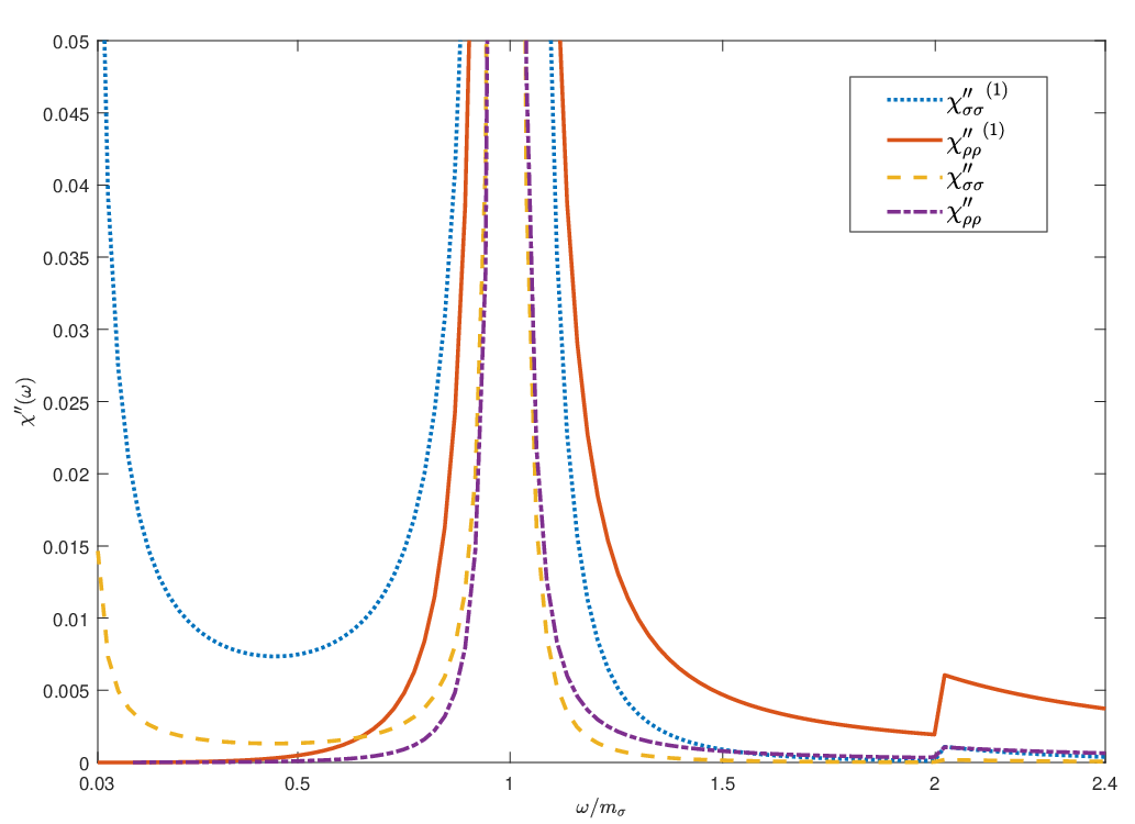
The spectral functions at ${\bf q}=0$ , $\chi^{\prime\prime}_{AB}(\omega)$ , can be numerically obtained. We obtain $\chi^{\prime\prime}_{\sigma\sigma}(\omega)$ and $\chi^{\prime\prime}_{\rho\rho}(\omega)$ for $j=2j_{c}$ . The susceptibilities are calculated using Eqs. (10), (38), (39), (43) and (44). The 1-loop level spectral functions of ${\chi^{\prime\prime}_{\sigma\sigma}}^{(1)}(\omega)$ and ${\chi^{\prime\prime}_{\rho\rho}}^{(1)}(\omega)$ are shown in Fig. 15.

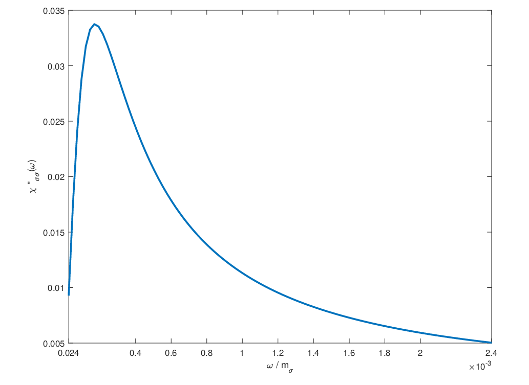
We also find from Fig. 15 that, in contrast with the conclusion of Ref. [15], the singularity of the spectral function of longitudinal susceptibility at $\omega\to 0$ does not damage the visibility of the peak at $\omega=m_{\sigma}$ . The plot at small values of $\omega$ , as magnified in Fig. 16, indicates that the spectral function is convergent.

The behaviour of the singularity at $\omega=0$ of longitudinal susceptibility is changed when 1PI summation is included, as can also be seen in the Eq. (C.2) of Ref. [15], which can be written as

\begin{split}&\chi_{\sigma\sigma}^{N=\infty}(q^{2})=\frac{1}{q^{2}+m_{\sigma}^{2}-\Pi_{\sigma}^{\rm 1PI}}.\end{split}

(45)

Even at 1-loop level and with only the leading contribution of large-N limit is included, i.e., $\Pi_{\sigma}^{\rm 1PI}=2U^{2}v^{2}\times\left(1/8q\right)$ , the spectral function can be written as

\begin{split}&{\chi^{\prime\prime}_{\sigma\sigma}}^{N=\infty,\;(1)}(\omega)=\frac{8m_{\sigma}^{2}\omega U}{m_{\sigma}^{4}\left(64\omega^{2}+U^{2}\right)-128m_{\sigma}^{2}\omega^{4}+64\omega^{6}}=\frac{8\omega}{m_{\sigma}^{2}U}+\mathcal{O}(\omega^{3}).\\ \end{split}

(46)

Therefore, although $\chi^{\prime\prime}_{\sigma\sigma}\sim\omega^{-1}$ at 1-loop level, in consistency with Ref. [15], we find that $\chi^{\prime\prime}_{\sigma\sigma}\sim\omega$ when 1PI summation is included.

We also find another small peak at about $2m_{\sigma}$ .

Similar to Ref. [4], we also show the spectral functions for $j$ ranging from $1.1j_{c}$ to $3.9j_{c}$ . The normalized spectral functions $\chi^{\prime\prime}_{\sigma\sigma}(\omega)$ and $\chi^{\prime\prime}_{\rho\rho}(\omega)$ are shown in Fig. 17 and Fig. 18, respectively. $\chi^{\prime\prime}_{\rho\rho}(\omega)$ is almost as same as $\chi^{\prime\prime}_{\sigma\sigma}(\omega)$ except that its peaks are a little wider.

We think that the disappearance of the peak of the spectral function when the weak interaction limit is approached, as observed in the experiment [4], cannot be explained by using the $O(2)$ model, because the $O(2)$ model is a relativistic model. As discussed in Ref. [7], the visibility of the Higgs mode depends on whether the model is relativistic or not. So we cannot reproduce the result of the experiment as long as we use a relativistic model in zero temperature limit.

The perturbation around $U/m_{\sigma}\sim 0$ is valid only when $U/m_{\sigma}\ll 1$ . $U/m_{\sigma}$ as a function of $j/j_{c}$ is shown in Fig. 19, where it can be seen that as $j$ decreases towards $j_{c}$ , $U/m_{\sigma}$ increases, invalidating the perturbation theory.

The monotonic decrease of $U/m_{\sigma}$ with the increase of $j/j_{c}$ is another evidence that the disappearance of the Higgs peak cannot be explained within the $O(2)$ model. With the increase of $j/j_{c}$ , $U/m_{\sigma}$ decreases, so the 1-loop or higher order contributions become less important, hence the spectral function approaches the delta function $\delta(\omega-m_{\sigma})$ .

V Conclusion

The Higgs mode observed in the two dimensional optical lattice [4] ended the debate whether the Higgs mode can be observed in the two dimensional neutral superfluid system. However, it was argued that, to reproduce the disappearance of the response, a theory between strong and weak interaction regimes is needed.

In this paper, we investigate the spectral function of the Higgs mode in $O(2)$ model. Differing from previous works, we calculate the spectral functions without using large-N expansion. The spectral function $\chi^{\prime\prime}_{\sigma\sigma}(\omega)$ and $\chi^{\prime\prime}_{\rho\rho}(\omega)$ are obtained in Eq. (39), as shown Fig. 17 and Fig. 18.

We argue that to use longitudinal susceptibility or scalar susceptibility is irrelevant to the visibility of the Higgs mode. We also find that the disappearance of the response with increase of $j/j_{c}$ cannot be explained within $O(2)$ model at zero temperature limit. We also find that there is a small peak in the spectral function at about $\omega\approx 2m_{\sigma}$ .

Appendix A Calculations of the Feynman diagrams

Calculations of the Feynman diagrams needed are listed below.

A.1 1-loop diagrams

A.1.1 Vacuum bubble diagrams

The vacuum bubble diagrams are drawn in (a) and (b) in Fig. 20,

\begin{split}&f^{(1)}_{a}=\mu^{\epsilon}\int\frac{d^{D}k}{(2\pi)^{D}}\frac{1}{k^{2}+m_{\sigma}^{2}},\;\;f^{(1)}_{b}=\mu^{\epsilon}\int\frac{d^{D}k}{(2\pi)^{D}}\frac{1}{k^{2}+\lambda^{2}}.\end{split}

(47)

Using DR, for $D\neq 2n$ ,

\begin{split}&G_{n}(m)\equiv\mu^{\epsilon}\int\frac{d^{D}k}{(2\pi)^{D}}\frac{1}{(k^{2}+m^{2})^{n}}=\frac{\mu^{\epsilon}}{(4\pi)^{\frac{D}{2}}}\frac{\Gamma(n-\frac{D}{2})}{\Gamma(n)}(m^{2})^{\frac{D}{2}-n}.\\ \end{split}

(48)

Unlike the cut-off regulator, in DR, the massless vacuum bubble diagrams vanish unless $D=2n$ , because the integral has dimension $[p]^{D-2n}$ while there is no external momentum or mass, hence no dimensional variable, the result can only be $0^{D-2n}$ [23]. Therefore for $D=3-\epsilon$ ,

\begin{split}&f^{(1)}_{a}=-\frac{m_{\sigma}}{4\pi},\;\;\;f^{(1)}_{b}=\begin{cases}0,\;\;\text{no IR divergence},\\ -\frac{\lambda}{4\pi},\;\;\text{with IR divergence}\end{cases}\\ .\\ \end{split}

(49)

When there is IR divergence, one should use $f_{b}^{(1)}=-\lambda/4\pi$ , for example, as for the diagrams in Fig. 21, which is nonzero because of the IR divergence.

A.1.2 Other 1-loop diagrams

Other 1-loop diagrams we need to calculate are drawn in (c) - (i) of Fig. 20, and are denoted as $f^{(1)}_{\alpha}(q^{2})$ , where $\alpha=c,d,e,f,g,h,i$ ,

\begin{split}&f^{(1)}_{c}(q^{2})=\int\frac{d^{3}k}{(2\pi)^{3}}\frac{1}{(k-q)^{2}+m_{\sigma}^{2}}\frac{1}{k^{2}+m_{\sigma}^{2}},\\ &f^{(1)}_{d}(q^{2})=\int\frac{d^{3}k}{(2\pi)^{3}}\frac{1}{(k-q)^{2}}\frac{1}{k^{2}},\\ &f^{(1)}_{e}(q^{2})=\int\frac{d^{3}k}{(2\pi)^{3}}\frac{1}{(k-q)^{2}}\frac{1}{k^{2}+m_{\sigma}^{2}},\\ &f^{(1)}_{f}(q^{2})=\int\frac{d^{3}k}{(2\pi)^{3}}\frac{1}{(k-q)^{2}+m_{\sigma}^{2}}\frac{1}{(k^{2}+m_{\sigma}^{2})^{2}},\\ &f^{(1)}_{g}(q^{2})=\int\frac{d^{3}k}{(2\pi)^{3}}\frac{1}{(k-q)^{2}+\lambda^{2}}\frac{1}{(k^{2}+\lambda^{2})^{2}},\\ &f^{(1)}_{h}(q^{2})=\int\frac{d^{3}k}{(2\pi)^{3}}\frac{1}{(k-q)^{2}+m_{\sigma}^{2}}\frac{1}{(k^{2}+\lambda^{2})^{2}},\\ &f^{(1)}_{i}(q^{2})=\int\frac{d^{3}k}{(2\pi)^{3}}\frac{1}{(k-q)^{2}}\frac{1}{(k^{2}+m_{\sigma}^{2})^{2}},\\ \end{split}

(50)

which are UV finite and are found to be

\begin{split}&f^{(1)}_{c}(q^{2})=\frac{1}{4\pi}\frac{\cot^{-1}\left(\frac{2m_{\sigma}}{q}\right)}{q},\;f^{(1)}_{d}(q^{2})=\frac{1}{8q},\;f^{(1)}_{e}(q^{2})=\frac{1}{4\pi}\frac{\tan^{-1}\left(\frac{q}{m_{\sigma}}\right)}{q},\\ &f^{(1)}_{f}(q^{2})=\frac{1}{4\pi}\frac{1}{2m_{\sigma}^{3}(t+4)},\;\;f^{(1)}_{g}(q^{2})=\frac{1}{4\pi}\frac{1}{2\lambda q^{2}},\\ &f^{(1)}_{h}(q^{2})=\frac{1}{4\pi}\left(\frac{1}{2\lambda m_{\sigma}^{2}(1+t)}-\frac{1}{m_{\sigma}^{3}(1+t)^{2}}\right),\;\;f^{(1)}_{i}(q^{2})=\frac{1}{4\pi}\frac{1}{2m_{\sigma}^{3}(1+t)},\\ \end{split}

(51)

where $t$ is defined as $t\equiv q^{2}/m_{\sigma}^{2}$ . The result $f^{(1)}_{d}$ is as same as in [15]. When $q^{2}=0$ , we have

\begin{split}&f^{(1)}_{c}(q^{2}=0)=\frac{1}{8\pi m_{\sigma}},\;\;f^{(1)}_{d}(q^{2}=0)=\frac{1}{8\pi\lambda},\;\;f^{(1)}_{e}(q^{2}=0)=\frac{1}{4\pi m_{\sigma}},\\ &f^{(1)}_{h}(q^{2}=0)=\frac{1}{4\pi}\left(\frac{1}{2\lambda m_{\sigma}^{2}}-\frac{1}{m_{\sigma}^{3}}\right),\;\;f^{(1)}_{i}(q^{2}=0)=\frac{1}{4\pi}\frac{1}{2m_{\sigma}^{3}},\\ \end{split}

(52)

A.2 2-loop diagrams

A.2.1 Sunset diagrams

The sunset diagrams are shown in Fig. 22. The diagrams in (a), (b), (c) and (d) of Fig. 22 are denoted as $f^{(2)}_{\alpha}(q^{2})$ , where $\alpha=a,b,c,d$ ,

\begin{split}&f^{(2)}_{a}(q^{2})=\mu^{\epsilon}\int\frac{d^{D}k_{1}}{(2\pi)^{D}}\int\frac{d^{D}k_{2}}{(2\pi)^{D}}\frac{1}{k_{1}^{2}}\frac{1}{k_{2}^{2}}\frac{1}{(k_{1}+k_{2}-q)^{2}},\\ &f^{(2)}_{b}(q^{2})=\mu^{\epsilon}\int\frac{d^{D}k_{1}}{(2\pi)^{D}}\int\frac{d^{D}k_{2}}{(2\pi)^{D}}\frac{1}{k_{1}^{2}}\frac{1}{k_{2}^{2}}\frac{1}{(k_{1}+k_{2}-q)^{2}+m_{\sigma}^{2}},\\ &f^{(2)}_{c}(q^{2})=\mu^{\epsilon}\int\frac{d^{D}k_{1}}{(2\pi)^{D}}\int\frac{d^{D}k_{2}}{(2\pi)^{D}}\frac{1}{k_{1}^{2}+m_{\sigma}^{2}}\frac{1}{k_{2}^{2}+m_{\sigma}^{2}}\frac{1}{(k_{1}+k_{2}-q)^{2}},\\ &f^{(2)}_{d}(q^{2})=\mu^{\epsilon}\int\frac{d^{D}k_{1}}{(2\pi)^{D}}\int\frac{d^{D}k_{2}}{(2\pi)^{D}}\frac{1}{k_{1}^{2}+m_{\sigma}^{2}}\frac{1}{k_{2}^{2}+m_{\sigma}^{2}}\frac{1}{(k_{1}+k_{2}-q)^{2}+m_{\sigma}^{2}},\\ \end{split}

(53)

which are UV divergent in $D=3-\epsilon$ .

The massless sunset diagrams with arbitrary powers of denominators are

\begin{split}&G_{n_{1},n_{2},n_{3}}(q^{2})=\mu^{\epsilon}\int\frac{d^{D}k_{1}}{(2\pi)^{D}}\int\frac{d^{D}k_{2}}{(2\pi)^{D}}\frac{1}{(k_{1}^{2})^{n_{1}}}\frac{1}{(k_{2}^{2})^{n_{2}}}\frac{1}{((k_{1}+k_{2}-q)^{2})^{n_{3}}}.\\ \end{split}

(54)

An efficient way to calculate this integral is to use the Fourier transformation [23]

\begin{split}&G_{n_{1},n_{2},n_{3}}(q^{2})=\frac{\mu^{\epsilon}}{(4\pi)^{D}}\frac{\Gamma(\frac{D}{2}-n_{1})\Gamma(\frac{D}{2}-n_{2})\Gamma(\frac{D}{2}-n_{3})}{\Gamma(n_{1})\Gamma(n_{2})\Gamma(n_{3})}\\ &\times\frac{\Gamma(n_{1}+n_{2}+n_{3}-D)}{\Gamma(\frac{3D}{2}-n_{1}-n_{2}-n_{3})}\frac{1}{(q^{2})^{n_{1}+n_{2}+n_{3}-D}}.\\ \end{split}

(55)

In $D=3-\epsilon$ , we need $f^{(2)}_{a}(q^{2})=G_{1,1,1}(q^{2})$ , and obtain

\begin{split}&f^{(2)}_{a}(q^{2})=\frac{1}{2(4\pi)^{2}}\left(N_{\rm UV}+\log\frac{\mu^{2}}{q^{2}}+3\right).\\ \end{split}

(56)

The sunset diagram with 1 internal mass can be calculated efficiently in Mellin-Barnes representation [24],

\begin{split}&f^{(2)}_{b}(q^{2})=\frac{\mu^{\epsilon}}{2\pi i}\int_{-i\infty}^{i\infty}dz\Gamma(1+z)\Gamma(-z)(m^{2})^{z}\\ &\times\int\frac{d^{D}k_{1}}{(2\pi)^{D}}\int\frac{d^{D}k_{2}}{(2\pi)^{D}}\frac{1}{k_{1}^{2}}\frac{1}{k_{2}^{2}}\frac{1}{((q-k_{1}-k_{2})^{2})^{1+z}}.\\ \end{split}

(57)

By using the massless sunset diagram Eq. (54), we obtain

\begin{split}&f^{(2)}_{b}(q^{2})=\mu^{\epsilon}\frac{(m_{\sigma}^{2})^{D-3}\Gamma^{2}(\frac{D}{2}-1)}{2\pi i(4\pi)^{D}}\\ &\times\int_{-i\infty}^{i\infty}dz\Gamma(-z)\frac{\Gamma(3-D+z)\Gamma(2-\frac{D}{2}+z)}{\Gamma(\frac{D}{2}+z)}t^{z}\\ &=\mu^{\epsilon}\frac{(m_{\sigma}^{2})^{D-3}\Gamma^{2}(\frac{D}{2}-1)}{(4\pi)^{D}}\frac{\Gamma(3-D)\Gamma(2-\frac{D}{2})}{\Gamma(\frac{D}{2})}\;_{2}F_{1}\left(\left.\begin{array}[]{c}3-D,2-\frac{D}{2}\\ \frac{D}{2}\end{array}\right|-t\right),\end{split}

(58)

where $t\equiv q^{2}/m_{\sigma}^{2}$ .

In $D=3-\epsilon$ , we use HypExp [25] to expand it around small $\epsilon$ , and find

\begin{split}&f^{(2)}_{b}(q^{2})=\frac{1}{2(4\pi)^{2}}\left(N_{\rm UV}+3+\log\frac{\mu^{2}}{q^{2}+m_{\sigma}^{2}}-\frac{2\tan^{-1}\left(\frac{q}{m_{\sigma}}\right)}{\frac{q}{m_{\sigma}}}\right),\\ \end{split}

(59)

Similar to the case with one internal mass, the sunset diagrams with two equal internal masses can be calculated in Mellin-Barnes representation. We obtain

\begin{split}&f^{(2)}_{c}(q^{2})\\ &=\mu^{\epsilon}\frac{(m_{\sigma}^{2})^{D-3}\Gamma(\frac{D}{2}-1)}{(4\pi)^{D}}\frac{\Gamma(3-D)\Gamma^{2}(2-\frac{D}{2})}{\Gamma(4-D)\Gamma(\frac{D}{2})}\\ &\times\;_{3}F_{2}\left(\left.\begin{array}[]{c}3-D,2-\frac{D}{2},1\\ \frac{5-D}{2},\frac{D}{2}\end{array}\right|-\frac{t}{4}\right).\\ \end{split}

(60)

When $D=3-\epsilon$ ,

\begin{split}&f^{(2)}_{c}(q^{2})=\frac{1}{2(4\pi)^{2}}\left(N_{\rm UV}+3+\log\frac{\mu^{2}}{4m_{\sigma}^{2}+q^{2}}-\frac{2\tan^{-1}\left(\frac{q}{2m_{\sigma}}\right)}{\frac{q}{2m_{\sigma}}}\right).\end{split}

(61)

We also obtain

\begin{split}&f^{(2)}_{d}(q^{2})=\mu^{\epsilon}\frac{\sqrt{\pi}(m_{\sigma}^{2})^{D-3}}{2(2\pi i)^{2}(4\pi)^{D}}\int_{\frac{D-1}{2}-i\infty}^{\frac{D-1}{2}+i\infty}dz_{1}\int_{\frac{D+1}{2}-i\infty}^{\frac{D+1}{2}+i\infty}dz_{2}t^{-z_{1}-z_{2}}\\ &\times\frac{4^{z_{1}}\Gamma(\frac{3-D}{2}-z_{1})\Gamma(\frac{1}{2}-z_{1})\Gamma(\frac{D-1}{2}-z_{1})\Gamma(\frac{3-D}{2}-z_{2})\Gamma(\frac{1}{2}-z_{2})\Gamma(z_{1}+z_{2})}{\Gamma(1-z_{1})\Gamma(\frac{D}{2}-z_{1}-z_{2})}.\\ \end{split}

(62)

We expand it around small $\epsilon$ first, with the help of MB.m package [26]. Then we use MBSums.m package [27], which depends on AMBRE.m package [28], to turn the integral into a summation. The result is

\begin{split}&f^{(2)}_{d}(q^{2})=\frac{1}{2(4\pi)^{2}}\left(N_{\rm UV}+3+\log\frac{\mu^{2}}{3m_{\sigma}^{2}}\right.\\ &\left.-\frac{3\tan^{-1}\left(\frac{1}{2}\left(\sqrt{t}-i\right)\right)}{\sqrt{t}}+\frac{i\left(\sqrt{t}+3i\right)\tan^{-1}\left(\frac{1}{2}\left(\sqrt{t}+i\right)\right)}{\sqrt{t}}+\frac{3\tan^{-1}\left(\frac{2\sqrt{t}}{t+3}\right)}{\sqrt{t}}\right.\\ &\left.-\frac{1}{2}\left(\log\left(2i\sqrt{t}+t+3\right)+\log\left(\frac{1}{9}\left(-2i\sqrt{t}+t+3\right)\right)+2\tanh^{-1}\left(\frac{1}{2}+\frac{i\sqrt{t}}{2}\right)\right)\right),\end{split}

(63)

with $t\equiv q^{2}\left./m_{\sigma}^{2}\right.$ .

In absence of external momenta,

\begin{split}&f^{(2)}_{a}(q^{2}=0)=\frac{1}{2(4\pi)^{2}}\left(N_{\rm UV}+1+\log\frac{\mu^{2}}{9\lambda^{2}}\right),\\ &f^{(2)}_{b}(q^{2}=0)=\frac{1}{2(4\pi)^{2}}\left(N_{\rm UV}+1+\log\frac{\mu^{2}}{m_{\sigma}^{2}}\right),\\ &f^{(2)}_{c}(q^{2}=0)=\frac{1}{2(4\pi)^{2}}\left(N_{\rm UV}+1+\log\frac{\mu^{2}}{4m_{\sigma}^{2}}\right),\\ &f^{(2)}_{d}(q^{2}=0)=\frac{1}{2(4\pi)^{2}}\left(N_{\rm UV}+1+\log\frac{\mu^{2}}{9m_{\sigma}^{2}}\right).\\ \end{split}

(64)

A.2.2 The second type of 2-loop diagrams.

The second type of 2-loop diagrams are shown in (e), (f), (g), (h), (i) and (j) of Fig. 23, and are denoted as $f^{(2)}_{\alpha}(q^{2})$ , with $\alpha=e,f,g,h,i,j$ ,

\begin{split}&f_{e}^{(2)}(q^{2})=\int\frac{d^{3}k_{1}}{(2\pi)^{3}}\int\frac{d^{3}k_{2}}{(2\pi)^{3}}\frac{1}{k_{1}^{2}}\frac{1}{(k_{1}-q)^{2}}\frac{1}{(k_{1}+k_{2})^{2}}\frac{1}{k_{2}^{2}+m_{\sigma}^{2}},\\ &f_{f}^{(2)}(q^{2})=\int\frac{d^{3}k_{1}}{(2\pi)^{3}}\int\frac{d^{3}k_{2}}{(2\pi)^{3}}\frac{1}{k_{1}^{2}+m_{\sigma}^{2}}\frac{1}{(k_{1}-q)^{2}}\frac{1}{(k_{1}+k_{2})^{2}}\frac{1}{k_{2}^{2}},\\ &f_{g}^{(2)}(q^{2})=\int\frac{d^{3}k_{1}}{(2\pi)^{3}}\int\frac{d^{3}k_{2}}{(2\pi)^{3}}\frac{1}{k_{1}^{2}+m_{\sigma}^{2}}\frac{1}{(k_{1}-q)^{2}+m_{\sigma}^{2}}\frac{1}{(k_{1}+k_{2})^{2}}\frac{1}{k_{2}^{2}},\\ &f_{h}^{(2)}(q^{2})=\int\frac{d^{3}k_{1}}{(2\pi)^{3}}\int\frac{d^{3}k_{2}}{(2\pi)^{3}}\frac{1}{k_{1}^{2}}\frac{1}{(k_{1}-q)^{2}+m_{\sigma}^{2}}\frac{1}{(k_{1}+k_{2})^{2}+m_{\sigma}^{2}}\frac{1}{k_{2}^{2}},\\ &f_{i}^{(2)}(q^{2})=\int\frac{d^{3}k_{1}}{(2\pi)^{3}}\int\frac{d^{3}k_{2}}{(2\pi)^{3}}\frac{1}{k_{1}^{2}+m_{\sigma}^{2}}\frac{1}{(k_{1}-q)^{2}}\frac{1}{(k_{1}+k_{2})^{2}+m_{\sigma}^{2}}\frac{1}{k_{2}^{2}+m_{\sigma}^{2}},\\ &f_{j}^{(2)}(q^{2})=\int\frac{d^{3}k_{1}}{(2\pi)^{3}}\int\frac{d^{3}k_{2}}{(2\pi)^{3}}\frac{1}{k_{1}^{2}+m_{\sigma}^{2}}\frac{1}{(k_{1}-q)^{2}+m_{\sigma}^{2}}\frac{1}{(k_{1}+k_{2})^{2}+m_{\sigma}^{2}}\frac{1}{k_{2}^{2}+m_{\sigma}^{2}},\\ \end{split}

(65)

which are UV finite.

$f_{e}^{(2)}(q^{2})$ can be efficiently calculated in Mellin-Barnes representation, by using MB.m package and MBSums.m package,

\begin{split}&f_{e}^{(2)}(q^{2})=\frac{1}{2(4\pi)^{2}m_{\sigma}^{2}}\frac{1}{t}\left(2\sqrt{t}\cot^{-1}(\sqrt{t})+\log(1+t)\right),\\ \end{split}

(66)

where $t\equiv q^{2}/m_{\sigma}^{2}$ .

We integrate $f_{f}^{(2)}(q^{2})$ , $f_{g}^{(2)}(q^{2})$ and $f_{h}^{(2)}(q^{2})$ by using the method in calculating the $C^{0}$ Passinal-Veltman function [29]. We take $f_{f}^{(2)}(q^{2})$ for example. In terms of the Feynman parameter, $f_{f}^{(2)}(q^{2})$ can be written as

\begin{split}&f_{f}^{(2)}(q^{2})=\frac{\Gamma^{2}(\frac{1}{2})}{(4\pi)^{3}}\int_{0}^{1}dx\int_{0}^{1-x}dy\frac{x^{-\frac{1}{2}}}{(1-x-y)m_{\sigma}^{2}+y(1-y)q^{2}}.\\ \end{split}

(67)

By making variable substitution $y\to(1-x)y$ , $x\to x^{2}$ , then $x\to x/y$ , and then $x\to x+y$ , the integral can be rewritten as

\begin{split}&f_{f}^{(2)}(q^{2})=\frac{2\Gamma^{2}(\frac{1}{2})}{(4\pi)^{3}m_{\sigma}^{2}}\int_{0}^{1}dy\int_{-y}^{0}dx\frac{1}{y(1-y+yt+x^{2}t+2xyt)},\\ \end{split}

(68)

where $t\equiv q^{2}/m_{\sigma}^{2}$ . Then by changing the order of integration over $x$ and $y$ , the integral can be written as

\begin{split}&f_{f}^{(2)}(q^{2})=\frac{2\Gamma^{2}(\frac{1}{2})}{(4\pi)^{3}m_{\sigma}^{2}}\int_{0}^{1}dx\int_{x}^{1}dy\frac{1}{y(1-y+yt+x^{2}t-2xyt)}.\\ \end{split}

(69)

Then we find

\begin{split}&f_{f}^{(2)}(q^{2})=\frac{1}{2(4\pi)^{2}m_{\sigma}^{2}}\frac{i}{2\sqrt{t}}\left\{\text{Li}_{2}\left(\frac{1}{1+\frac{i}{\sqrt{t}}}\right)-\text{Li}_{2}\left(\frac{1}{1-\frac{i}{\sqrt{t}}}\right)+\text{Li}_{2}\left(\frac{1}{i\sqrt{t}+1}\right)\right.\\ &\left.-\text{Li}_{2}\left(\frac{1}{1-i\sqrt{t}}\right)-\frac{i\pi}{2}\log(t+1)+i\log(t)\tan^{-1}\left(\sqrt{t}\right)\right\}.\\ \end{split}

(70)

Similarly we find

\begin{split}&f_{g}^{(2)}(q^{2})=\frac{1}{2(4\pi)^{2}m_{\sigma}^{2}}\frac{1}{2\sqrt{t}}\left\{\frac{1}{2}\left[-2i\log\left(1-\frac{i}{\sqrt{t}}\right)\log\left(\frac{i}{\sqrt{t}}\right)+2i\log\left(1+\frac{i}{\sqrt{t}}\right)\log\left(-\frac{i}{\sqrt{t}}\right)\right.\right.\\ &\left.\left.+2i\log\left(\frac{\sqrt{t}-i}{\sqrt{t}-2i}\right)\log\left(-\frac{i}{\sqrt{t}-2i}\right)-2i\log\left(\frac{\sqrt{t}+i}{\sqrt{t}+2i}\right)\log\left(\frac{i}{\sqrt{t}+2i}\right)\right.\right.\\ &\left.\left.+2\pi\log\left(2-i\sqrt{t}\right)+\pi\left(\log\left(16i\left(\sqrt{t}+i\right)t\right)-2\log\left(\sqrt{t}-\sqrt{t+4}+2i\right)\right)\right.\right.\\ &\left.\left.+i\left(\pi^{2}+\log\left(-1+i\sqrt{t}\right)\left(\log(t)+2\log\left(-8+4i\sqrt{t}\right)-2\log\left(\sqrt{t}-\sqrt{t+4}+2i\right)\right)\right)\right.\right.\\ &\left.\left.-\log\left(1+i\sqrt{t}\right)\left(2i\log\left(2+i\sqrt{t}\right)+2i\log\left(-\frac{4\sqrt{t}}{-\sqrt{t}+\sqrt{t+4}+2i}\right)\right.\right.\right.\\ &\left.\left.\left.-2i\log\left(\sqrt{t}+\sqrt{t+4}-2i\right)+3\pi\right)+2\left(\pi+i\log\left(-1+i\sqrt{t}\right)\right)\log\left(-\frac{1}{\sqrt{t}+\sqrt{t+4}+2i}\right)\right]\right.\\ &\left.-i\left[\text{Li}_{2}\left(-i\sqrt{t}\right)-\text{Li}_{2}\left(i\sqrt{t}\right)-2\text{Li}_{2}\left(\frac{-i+\sqrt{t}}{-2i+\sqrt{t}}\right)+2\text{Li}_{2}\left(\frac{i+\sqrt{t}}{2i+\sqrt{t}}\right)\right.\right.\\ &\left.\left.+\text{Li}_{2}\left(\frac{2i}{2i+\sqrt{t}-\sqrt{t+4}}\right)-\text{Li}_{2}\left(\frac{2\left(i+\sqrt{t}\right)}{2i+\sqrt{t}-\sqrt{t+4}}\right)-\text{Li}_{2}\left(\frac{2i}{2i-\sqrt{t}+\sqrt{t+4}}\right)\right.\right.\\ &\left.\left.+\text{Li}_{2}\left(\frac{2i-2\sqrt{t}}{2i-\sqrt{t}+\sqrt{t+4}}\right)+\text{Li}_{2}\left(\frac{2\left(-i+\sqrt{t}\right)}{-2i+\sqrt{t}+\sqrt{t+4}}\right)-\text{Li}_{2}\left(-\frac{2i}{-2i+\sqrt{t}+\sqrt{t+4}}\right)\right.\right.\\ &\left.\left.+\text{Li}_{2}\left(\frac{2i}{2i+\sqrt{t}+\sqrt{t+4}}\right)-\text{Li}_{2}\left(\frac{2\left(i+\sqrt{t}\right)}{2i+\sqrt{t}+\sqrt{t+4}}\right)\right]\right\},\end{split}

(71)

\begin{split}&f_{h}^{(2)}(q^{2})=\frac{1}{2(4\pi)^{2}m_{\sigma}^{2}}\frac{1}{\sqrt{t}(t+1)}\left\{-2(t+1)\cot^{-1}\left(\frac{2}{\sqrt{t}}\right)-2\tan^{-1}\left(\sqrt{t}\right)\right.\\ &\left.+i\left[(t+1)\log\left(-\frac{\left(\sqrt{t}+i\right)^{2}}{t+1}\right)-i\sqrt{t}\log(t+4)+\log\left(\frac{t-i\sqrt{t}+2}{t+i\sqrt{t}+2}\right)\right]\right\}\end{split}

(72)

$f_{i}^{(2)}(q^{2})$ and $f_{j}^{(2)}(q^{2})$ are more difficult to calculate, we take $f_{j}^{(2)}(q^{2})$ for example, it can written as

\begin{split}&f_{j}^{(2)}(q^{2})=f_{g}^{(2)}(q^{2})-\frac{1}{2(4\pi)^{2}m_{\sigma}^{2}}2\left(-\frac{\log(3)\cot^{-1}\left(\frac{2}{\sqrt{t}}\right)}{2\sqrt{t}}+f_{j_{1}}(t)\right),\\ &f_{j_{1}}(t)=\int_{0}^{1}dx\frac{\coth^{-1}\left(2\sqrt{\frac{t(x-1)x-1}{x(t(x-1)+3)-4}}\right)}{2\sqrt{1-t(x-1)x}},\\ \end{split}

(73)

where

\begin{split}&f_{j_{1}}(t)=\frac{1}{\sqrt{t}}f_{j_{2}}(u),\;\;\;f_{j_{2}}(u)=\int_{0}^{1}dx\frac{\coth^{-1}\left(2\sqrt{\frac{(x-1)x-u}{x((x-1)+3u)-4u}}\right)}{2\sqrt{u-(x-1)x}},\\ \end{split}

(74)

with $u\equiv 1/t$ .

It can be written that

\begin{split}&f_{j_{2}}(u)=\int_{0}^{u}\left(\int_{0}^{1}dx\frac{\partial}{\partial u}\frac{\coth^{-1}\left(2\sqrt{\frac{(x-1)x-u}{x((x-1)+3u)-4u}}\right)}{2\sqrt{u-(x-1)x}}\right)+C,\\ \end{split}

(75)

where $C$ is a constant and can be obtained by comparing the result with

\begin{split}&f_{j_{2}}(u=0)=\int_{0}^{1}dx\frac{\coth^{-1}\left(2\sqrt{\frac{(x-1)x}{x((x-1))}}\right)}{2\sqrt{(1-x)x}}.\\ \end{split}

(76)

Eq. (75) is easier to integrate, one can integrate over $x$ and then over $u$ to obtain $f_{j_{2}}$ .

Finally

\begin{split}&f_{i}^{(2)}(q^{2})=f_{f}^{(2)}(q^{2})-\frac{1}{2(4\pi)^{2}m_{\sigma}^{2}}\frac{i}{2\sqrt{t}}\left\{-\log\left(\frac{1}{\sqrt{t}}-\frac{i}{2}\right)\log\left(\frac{3\left(\sqrt{t}+i\right)}{\sqrt{t}-i}\right)\right.\\ &\left.+\text{Li}_{2}\left(-1+\frac{2i}{\sqrt{t}}\right)-\text{Li}_{2}\left(-1-\frac{2i}{\sqrt{t}}\right)+\text{Li}_{2}\left(\frac{1}{3}+\frac{2i}{3\sqrt{t}}\right)-\text{Li}_{2}\left(\frac{1}{3}-\frac{2i}{3\sqrt{t}}\right)\right.\\ &\left.+\log(3)\left[\log(t+1)+\log\left(\frac{1}{\sqrt{t}}+\frac{i}{2}\right)-2\log\left(1+i\sqrt{t}\right)\right]\right.\\ &\left.-2i\log\left(\frac{2}{3}\left(\frac{2}{\sqrt{t}}+i\right)\right)\cot^{-1}\left(\sqrt{t}\right)\right\},\\ \end{split}

(77)

\begin{split}&f_{j}^{(2)}(q^{2})=f_{g}^{(2)}(q^{2})-\frac{1}{2(4\pi)^{2}m_{\sigma}^{2}}\frac{1}{\sqrt{t}}\left\{\frac{1}{8}i\left[4{\rm Re}(\text{Li}_{2}(3))-4\text{Li}_{2}(3)-4i\log\left(\frac{t}{t+4}\right)\tan^{-1}\left(\frac{2\sqrt{t}}{t+3}\right)\right.\right.\\ &\left.\left.-2\log\left(\frac{1}{\sqrt{t}}+\frac{i}{2}\right)\log\left(-\frac{3\left(t+2i\sqrt{t}+3\right)}{5\left(t-2i\sqrt{t}+3\right)}\right)+\log(9)\log\left(\frac{1}{3}+\frac{2i}{3\left(\sqrt{t}-i\right)}\right)\right.\right.\\ &\left.\left.+4i\log\left(\frac{1}{\sqrt{t}+2i}+\frac{i}{2}\right)\tan^{-1}\left(\frac{3}{\sqrt{t}}\right)-4i\log\left(3\left(\frac{1}{\sqrt{t}+2i}+\frac{i}{2}\right)\right)\cot^{-1}\left(\sqrt{t}\right)\right.\right.\\ &\left.\left.+2\log\left(\frac{1}{\sqrt{t}}-\frac{i}{2}\right)\left(\log\left(\frac{3}{5}\left(-1+\frac{6i}{\sqrt{t}+3i}\right)\right)+2i\tan^{-1}\left(\frac{3}{\sqrt{t}}\right)\right)+8i\log(3)\cot^{-1}\left(\frac{2}{\sqrt{t}}\right)\right.\right.\\ &\left.\left.+2\left(-\log(t+4)+2\log\left(2+i\sqrt{t}\right)\right)\left(\log\left(-\frac{3}{5}+\frac{6i}{5\left(\sqrt{t}+3i\right)}\right)+2\coth^{-1}\left(2-i\sqrt{t}\right)\right)\right.\right.\\ &\left.\left.+\pi^{2}+\log^{2}(3)+\log^{2}(5)+2i\pi\log\left(\frac{20}{9}\right)\right]+\frac{1}{4}\left[-i\text{Li}_{2}\left(2i\sqrt{\frac{1}{t}}-1\right)-i\text{Li}_{2}\left(6i\sqrt{\frac{1}{t}}+3\right)\right.\right.\\ &\left.\left.-i\text{Li}_{2}\left(\frac{2}{3}i\sqrt{\frac{1}{t}}+\frac{1}{3}\right)+i\text{Li}_{2}\left(\frac{6}{5}i\sqrt{\frac{1}{t}}+\frac{3}{5}\right)+i\text{Li}_{2}\left(-2i\sqrt{\frac{1}{t}}-1\right)+i\text{Li}_{2}\left(3-6i\sqrt{\frac{1}{t}}\right)\right.\right.\\ &\left.\left.+i\text{Li}_{2}\left(\frac{1}{3}-\frac{2}{3}i\sqrt{\frac{1}{t}}\right)-i\text{Li}_{2}\left(\frac{3}{5}-\frac{6}{5}i\sqrt{\frac{1}{t}}\right)\right]-\frac{1}{12}i\left[3\text{Li}_{2}\left(e^{2i\tan^{-1}\left(\frac{1}{2\sqrt{\frac{1}{t}}}\right)+2\tanh^{-1}\left(\frac{1}{2}\right)}\right)\right.\right.\\ &\left.\left.+3\text{Li}_{2}\left(e^{2i\tan^{-1}\left(\frac{1}{2\sqrt{\frac{1}{t}}}\right)-2\tanh^{-1}\left(\frac{1}{2}\right)}\right)-3\text{Li}_{2}\left(e^{2i\tan^{-1}\left(\frac{1}{2\sqrt{\frac{1}{t}}}\right)+2\tanh^{-1}\left(\frac{3}{2}\right)}\right)\right.\right.\\ &\left.\left.-3\text{Li}_{2}\left(e^{2i\tan^{-1}\left(\frac{1}{2\sqrt{\frac{1}{t}}}\right)-2\tanh^{-1}\left(\frac{3}{2}\right)}\right)\right]\right\}.\\ \end{split}

(78)

When $q^{2}=0$ ,

\begin{split}&f_{e}^{(2)}{(q^{2}=0)}=\frac{1}{2(4\pi)^{2}m_{\sigma}^{2}}\left(\frac{m_{\sigma}}{\lambda}-2\right),\;\;\;f_{f}^{(2)}{(q^{2}=0)}=-\frac{1}{2(4\pi)^{2}m_{\sigma}^{2}}\log\left(9\frac{\lambda^{2}}{m_{\sigma}^{2}}\right),\\ &f_{g}^{(2)}{(q^{2}=0)}=\frac{1}{2(4\pi)^{2}m_{\sigma}^{2}},\;\;\;f_{h}^{(2)}{(q^{2}=0)}=\frac{1}{2(4\pi)^{2}m_{\sigma}^{2}}\log(4),\\ &f_{i}^{(2)}{(q^{2}=0)}=\frac{1}{2(4\pi)^{2}m_{\sigma}^{2}}\log\left(\frac{9}{4}\right),\;\;\;f_{j}^{(2)}{(q^{2}=0)}=\frac{1}{2(4\pi)^{2}m_{\sigma}^{2}}\frac{1}{3}.\\ \end{split}

(79)

Note that the diagrams (e), (g), (j) of Fig. 24 are $f_{e}^{(2)}(q^{2}=0)$ , $f_{g}^{(2)}(q^{2}=0)$ and $f_{j}^{(2)}(q^{2}=0)$ .

Compared with the result of numerical integration, note that in making analytical continuation $|q|\to\sqrt{-(\omega+i\epsilon)^{2}}$ , one should use $\left(f_{h}((q^{2})^{*})\right)^{*}$ instead of $f_{h}(q^{2})$ .

A.2.3 Integral by part recursive relations

The remaining diagrams are more difficult to calculate. We use the integral-by-part (IBP) recursive relations [30]. For convenience, we establish some definitions. The 2-loop diagrams can be written as

\begin{split}&f(n_{1},n_{2},n_{3},n_{4},n_{5})=\int\frac{d^{D}k_{1}}{(2\pi)^{D}}\int\frac{d^{D}k_{2}}{(2\pi)^{D}}\frac{1}{(k_{1}^{2}+m_{3}^{2})^{n_{3}}}\\ &\times\frac{1}{((k_{1}+q)^{2}+m_{1}^{2})^{n_{1}}}\frac{1}{((k_{2}-k_{1})^{2}+m_{5}^{2})^{n_{5}}}\frac{1}{(k_{2}^{2}+m_{4}^{2})^{n_{4}}}\frac{1}{((k_{2}+q)^{2}+m_{2}^{2})^{n_{2}}}.\end{split}

(80)

We define the ${\bf 1}^{\pm}$ operator as

\begin{split}&{\bf 1}^{\pm}f(n_{1},n_{2},n_{3},n_{4},n_{5})=f(n_{1}\pm 1,n_{2},n_{3},n_{4},n_{5}),\\ \end{split}

(81)

and ${\bf 2}^{\pm}$ , ${\bf 3}^{\pm}$ , ${\bf 4}^{\pm}$ and ${\bf 5}^{\pm}$ similarly.

With $k_{2}\cdot\frac{\partial}{\partial k_{2}}$ , $k_{1}\cdot\frac{\partial}{\partial k_{2}}$ and $q\cdot\frac{\partial}{\partial k_{2}}$ acting on $f$ , we obtain the IBP relations

\begin{split}&0=\left(D-n_{5}-2n_{4}-n_{2}-n_{5}({\bf 4}^{-}-{\bf 3}^{-}+m_{3}^{2}-m_{4}^{2}-m_{5}^{2}){\bf 5}^{+}\right.\\ &\left.+2n_{4}m_{4}^{2}{\bf 4}^{+}-n_{2}({\bf 4}^{-}-m_{4}^{2}-m_{2}^{2}-q^{2}){\bf 2}^{+}\right)f,\\ &0=\left(n_{5}-n_{4}-n_{5}({\bf 4}^{-}-{\bf 3}^{-}+m_{3}^{2}-m_{4}^{2}+m_{5}^{2}){\bf 5}^{+}-n_{4}({\bf 3}^{-}-{\bf 5}^{-}+m_{5}^{2}-m_{3}^{2}-m_{4}^{2}){\bf 4}^{+}\right.\\ &\left.-n_{2}({\bf 4}^{-}+{\bf 1}^{-}-{\bf 5}^{-}+m_{5}^{2}-m_{1}^{2}-m_{4}^{2}-q^{2}){\bf 2}^{+}\right)f,\\ &0=\left(n_{4}-n_{2}-n_{5}({\bf 2}^{-}+{\bf 3}^{-}-{\bf 1}^{-}-{\bf 4}^{-}+m_{1}^{2}+m_{4}^{2}-m_{2}^{2}-m_{3}^{2}){\bf 5}^{+}\right.\\ &\left.-n_{4}({\bf 2}^{-}+m_{4}^{2}-m_{2}^{2}-q^{2}){\bf 4}^{+}-n_{2}(-{\bf 4}^{-}+m_{4}^{2}-m_{2}^{2}+q^{2}){\bf 2}^{+}\right)f.\\ \end{split}

(82)

For example, the substraction of the first two equations in Eq. (82) is one of the triangle rules [23]. When $n_{i}=1$ and $D=3$ ,

\begin{split}&0=\left(-1+2m_{5}^{2}{\bf 5}^{+}+({\bf 3}^{-}-{\bf 5}^{-}+m_{5}^{2}-m_{3}^{2}+m_{4}^{2}){\bf 4}^{+}\right.\\ &\left.+({\bf 1}^{-}-{\bf 5}^{-}+m_{5}^{2}-m_{1}^{2}+m_{2}^{2}){\bf 2}^{+}\right)f(1,1,1,1,1).\\ \end{split}

(83)

Most of the remaining diagrams are calculated with the help of IBP relations.

A.2.4 The third type of 2-loop diagrams

The second type of 2-loop diagrams are shown in Fig. 25. The diagrams in (k), (l), (m), (n), (o) and (p) of Fig. 25 are denoted as $f^{(2)}_{\alpha}(q^{2})$ , where $\alpha=k,l,m,n,o,p$ ,

\begin{split}&f^{(2)}_{k}(q^{2})=\int\frac{d^{3}k_{1}}{(2\pi)^{3}}\int\frac{d^{3}k_{2}}{(2\pi)^{3}}\frac{1}{(k_{1}^{2}+\lambda^{2})^{2}}\frac{1}{(k_{1}-q)^{2}+m_{\sigma}^{2}}\frac{1}{(k_{1}-k_{2})^{2}+m_{\sigma}^{2}}\frac{1}{k_{2}^{2}+\lambda^{2}},\\ &f^{(2)}_{l}(q^{2})=\int\frac{d^{3}k_{1}}{(2\pi)^{3}}\int\frac{d^{3}k_{2}}{(2\pi)^{3}}\frac{1}{(k_{1}^{2}+m_{\sigma}^{2})^{2}}\frac{1}{(k_{1}-q)^{2}}\frac{1}{(k_{1}-k_{2})^{2}+m_{\sigma}^{2}}\frac{1}{k_{2}^{2}+m_{\sigma}^{2}},\\ &f^{(2)}_{m}(q^{2})=\int\frac{d^{3}k_{1}}{(2\pi)^{3}}\int\frac{d^{3}k_{2}}{(2\pi)^{3}}\frac{1}{(k_{1}^{2}+m_{\sigma}^{2})^{2}}\frac{1}{(k_{1}-q)^{2}}\frac{1}{(k_{1}-k_{2})^{2}}\frac{1}{k_{2}^{2}},\\ &f^{(2)}_{n}(q^{2})=\int\frac{d^{3}k_{1}}{(2\pi)^{3}}\int\frac{d^{3}k_{2}}{(2\pi)^{3}}\frac{1}{(k_{1}^{2}+\lambda^{2})^{2}}\frac{1}{(k_{1}-q)^{2}+\lambda^{2}}\frac{1}{(k_{1}-k_{2})^{2}+m_{\sigma}^{2}}\frac{1}{k_{2}^{2}+\lambda^{2}},\\ &f^{(2)}_{o}(q^{2})=\int\frac{d^{3}k_{1}}{(2\pi)^{3}}\int\frac{d^{3}k_{2}}{(2\pi)^{3}}\frac{1}{(k_{1}^{2}+m_{\sigma}^{2})^{2}}\frac{1}{(k_{1}-q)^{2}+m_{\sigma}^{2}}\frac{1}{(k_{1}-k_{2})^{2}+m_{\sigma}^{2}}\frac{1}{k_{2}^{2}+m_{\sigma}^{2}},\\ &f^{(2)}_{p}(q^{2})=\int\frac{d^{3}k_{1}}{(2\pi)^{3}}\int\frac{d^{3}k_{2}}{(2\pi)^{3}}\frac{1}{(k_{1}^{2}+m_{\sigma}^{2})^{2}}\frac{1}{(k_{1}-q)^{2}+m_{\sigma}^{2}}\frac{1}{(k_{1}-k_{2})^{2}}\frac{1}{k_{2}^{2}},\\ \end{split}

(84)

which are UV finite. $f_{k}^{(2)}$ in Eq. (84) and $f_{h}^{(2)}$ in Eq. (65) can be rewritten as

\begin{split}&f^{(2)}_{k}(q^{2})=\int\frac{d^{3}k_{1}}{(2\pi)^{3}}\int\frac{d^{3}k_{2}}{(2\pi)^{3}}\frac{1}{k_{1}^{2}+\lambda^{2}}\frac{1}{(k_{1}-k_{2})^{2}+m_{\sigma}^{2}}\frac{1}{(k_{2}^{2}+\lambda^{2})^{2}}\frac{1}{(k_{2}-q)^{2}+m_{\sigma}^{2}},\\ &f^{(2)}_{h}(q^{2})=\int\frac{d^{3}k_{1}}{(2\pi)^{3}}\int\frac{d^{3}k_{2}}{(2\pi)^{3}}\frac{1}{k_{1}^{2}+\lambda^{2}}\frac{1}{(k_{2}-k_{1})^{2}+m_{\sigma}^{2}}\frac{1}{k_{2}^{2}+\lambda^{2}}\frac{1}{(k_{2}+q)^{2}+m_{\sigma}^{2}}.\\ \end{split}

(85)

We find, at order $\mathcal{O}(\lambda^{0})$ ,

\begin{split}&\left(-1+2m_{\sigma}^{2}{\bf 5}^{+}+({\bf 3}^{-}-{\bf 5}^{-}+m_{\sigma}^{2}){\bf 4}^{+}+(({\bf 1}^{-}-m_{1}^{2})-{\bf 5}^{-}+2m_{\sigma}^{2}){\bf 2}^{+}\right)f_{h}^{(2)}=0,\\ \end{split}

(86)

where

\begin{split}&{\bf 4}^{+}f_{h}^{(2)}=f_{k}^{(2)},\\ &({\bf 1}^{-}-m_{1}^{2}){\bf 2}^{+}f_{h}^{(2)}\\ &=\int\frac{d^{3}k_{1}}{(2\pi)^{3}}\int\frac{d^{3}k_{2}}{(2\pi)^{3}}\frac{k_{1}^{2}+2k_{1}\cdot q+q^{2}}{k_{1}^{2}}\frac{1}{(k_{2}-k_{1})^{2}+m_{\sigma}^{2}}\frac{1}{k_{2}^{2}}\frac{1}{((k_{2}+q)^{2}+m_{\sigma}^{2})^{2}}.\\ \end{split}

(87)

All the other integrals in Eq. (86) can be calculated to obtain $f_{k}^{(2)}$ . Using this procedure, we find

\begin{split}&f_{k}^{(2)}(q^{2})=\frac{1}{m_{\sigma}^{2}}f_{h}^{(2)}(q^{2})+\frac{1}{(4\pi)^{3}m_{\sigma}^{4}}\left\{\frac{2\pi m_{\sigma}}{\lambda(t+1)}+\frac{2\pi}{3\sqrt{t}(t+1)^{3}}\left[-\sqrt{t}(t(3t+5)+6)\log(t+4)\right.\right.\\ &\left.\left.+2\left(-(t+5)\left(t^{2}+t+1\right)\cot^{-1}\left(\frac{t+2}{\sqrt{t}}\right)+(2t+3)\left(-\sqrt{t}\right)(t+1)\right.\right.\right.\\ &\left.\left.\left.-(3t(t(t+2)+2)-1)\tan^{-1}\left(\sqrt{t}\right)+3(t+1)^{3}\cot^{-1}\left(\frac{2}{\sqrt{t}}\right)\right)\right]\right\},\end{split}

(88)

where $t\equiv q^{2}/m_{\sigma}^{2}$ .

Similarly, we find

\begin{split}&f_{l}^{(2)}(q^{2})=\frac{1}{2m_{\sigma}^{2}}f_{i}^{(2)}(q^{2})+\frac{\pi}{(4\pi)^{3}m_{\sigma}^{4}}\left\{\frac{(\log(81)-2\log(t+4))}{2(1+t)}-\frac{\csc^{-1}\left(\sqrt{\frac{1}{t}+1}\right)}{\sqrt{t}}\right.\\ &\left.-\frac{\tan^{-1}\left(\frac{\sqrt{t}}{2}\right)}{\sqrt{t}}-\frac{\left(\tan^{-1}\left(\frac{t-1}{2\sqrt{t}}\right)+\tan^{-1}\left(\frac{4-t}{4\sqrt{t}}\right)\right)}{6\sqrt{t}}\right\},\end{split}

(89)

\begin{split}&f_{m}^{(2)}(q^{2})=\frac{1}{2m_{\sigma}^{2}}f_{f}^{(2)}(q^{2})+\frac{1}{(4\pi)^{3}m_{\sigma}^{4}}\frac{\pi\log\left(\frac{1}{t}\right)}{t+1},\end{split}

(90)

\begin{split}&f_{n}^{(2)}(q^{2})=-\frac{1}{(4\pi)^{3}m_{\sigma}^{4}}\frac{\pi}{6t^{2}}\left\{t\left(-\frac{12m_{\sigma}}{\lambda}+\pi\sqrt{t}+16\right)\right.\\ &\left.+2t^{3/2}\left(2\tan^{-1}\left(\sqrt{t}\right)-3\tan^{-1}\left(\frac{t-1}{2\sqrt{t}}\right)\right)-4\log(t+1)\right\},\end{split}

(91)

\begin{split}&f_{o}^{(2)}(q^{2})=\frac{1}{2m_{\sigma}^{2}}f_{j}^{(2)}(q^{2})+\frac{\pi}{(4\pi)^{3}m_{\sigma}^{4}}\left\{\frac{\tan^{-1}\left(\frac{t+3}{2\sqrt{t}}\right)}{\sqrt{t}}-\frac{\cot^{-1}\left(\frac{2}{\sqrt{t}}\right)}{\sqrt{t}}-\frac{\tan^{-1}\left(\frac{3-t}{4\sqrt{t}}\right)}{\sqrt{t}}\right.\\ &\left.-\frac{(t+2)\left[2\log\left(\frac{t+9}{9}\right)+\sqrt{t}\left((t+4)\left(2\tan^{-1}\left(-\frac{3}{\sqrt{t}}\right)+\pi\right)+i(t+3)\log\left(-1+\frac{6i}{\sqrt{t}+3i}\right)\right)\right]}{2t(t+4)}\right.\\ &\left.+\frac{\tan^{-1}\left(\frac{t+3}{2\sqrt{t}}\right)+\tan^{-1}\left(\frac{t-3}{4\sqrt{t}}\right)-2\cot^{-1}\left(\frac{2}{\sqrt{t}}\right)}{6\sqrt{t}}\right\},\end{split}

(92)

\begin{split}&f_{p}^{(2)}(q^{2})=\frac{1}{2(4\pi)^{3}m_{\sigma}^{4}t^{2}}\left\{\frac{1}{2}it^{3/2}\left[-\text{Li}_{2}\left(i\sqrt{t}+1\right)+\text{Li}_{2}\left(\frac{1}{i\sqrt{t}+2}\right)+\text{Li}_{2}\left(1-i\sqrt{t}\right)\right.\right.\\ &\left.\left.-\text{Li}_{2}\left(\frac{1}{2-i\sqrt{t}}\right)+\text{Li}_{2}\left(1+\frac{1}{i\sqrt{t}-2}\right)-\text{Li}_{2}\left(1+\frac{1}{-i\sqrt{t}-2}\right)+\text{Li}_{2}\left(\frac{2i}{2i+\sqrt{t}-\sqrt{t+4}}\right)\right.\right.\\ &\left.\left.-\text{Li}_{2}\left(\frac{2\left(i+\sqrt{t}\right)}{2i+\sqrt{t}-\sqrt{t+4}}\right)-\text{Li}_{2}\left(\frac{2i}{2i-\sqrt{t}+\sqrt{t+4}}\right)+\text{Li}_{2}\left(\frac{2i-2\sqrt{t}}{2i-\sqrt{t}+\sqrt{t+4}}\right)\right.\right.\\ &\left.\left.+\text{Li}_{2}\left(\frac{2\left(-i+\sqrt{t}\right)}{-2i+\sqrt{t}+\sqrt{t+4}}\right)-\text{Li}_{2}\left(-\frac{2i}{-2i+\sqrt{t}+\sqrt{t+4}}\right)+\text{Li}_{2}\left(\frac{2i}{2i+\sqrt{t}+\sqrt{t+4}}\right)\right.\right.\\ &\left.\left.-\text{Li}_{2}\left(\frac{2\left(i+\sqrt{t}\right)}{2i+\sqrt{t}+\sqrt{t+4}}\right)\right]-\frac{t(t+2)\log(t+1)}{t+4}+\frac{t^{3/2}}{4(t+4)}\left[-\pi(t+4)\log\left(\frac{1}{t}+1\right)\right.\right.\\ &\left.\left.+2i(t+4)\log\left(-\sqrt{t}+i\right)+4i\log\left(\sqrt{t}+i\right)-2(t+4)\log(t)\cot^{-1}\left(\sqrt{t}\right)\right.\right.\\ &\left.\left.+(t+6)\left(\pi-2i\log\left(1+i\sqrt{t}\right)\right)\right]\right\},\end{split}

(93)

where $t\equiv q^{2}/m_{\sigma}^{2}$ .

We also obtain

\begin{split}&f_{k}^{(2)}(q^{2}=0)=\frac{1}{2(4\pi)^{2}m_{\sigma}^{4}}\left(-2+\frac{m_{\sigma}}{\lambda}-\log(4)\right),\;f_{l}^{(2)}(q^{2}=0)=\frac{1}{2(4\pi)^{2}m_{\sigma}^{4}}\left(2\log\left(\frac{3}{2}\right)-\frac{1}{3}\right),\\ &f_{m}^{(2)}(q^{2}=0)=\frac{1}{2(4\pi)^{2}m_{\sigma}^{4}}\left(-1-2\log(3)-\log\left(\frac{\lambda^{2}}{m_{\sigma}^{2}}\right)\right).\\ \end{split}

(94)

A.2.5 The fourth type of 2-loop diagrams.

The second type of 2-loop diagrams are shown in Fig. 26. The diagrams in (q), (r), (s), (t), (u) and (v) of Fig. 26 are denoted as $f^{(2)}_{\alpha}(q^{2})$ , with $\alpha=q,r,s,t,u,v$ ,

\begin{split}&f_{q}^{(2)}(q^{2})=\int\frac{d^{3}k_{1}}{(2\pi)^{3}}\int\frac{d^{3}k_{2}}{(2\pi)^{3}}\frac{1}{k_{1}^{2}+m_{\sigma}^{2}}\frac{1}{(k_{1}+q)^{2}+m_{\sigma}^{2}}\frac{1}{(k_{1}-k_{2})^{2}+m_{\sigma}^{2}}\\ &\times\frac{1}{k_{2}^{2}+m_{\sigma}^{2}}\frac{1}{(k_{2}+q)^{2}+m_{\sigma}^{2}},\\ &f_{r}^{(2)}(q^{2})=\int\frac{d^{3}k_{1}}{(2\pi)^{3}}\int\frac{d^{3}k_{2}}{(2\pi)^{3}}\frac{1}{k_{1}^{2}}\frac{1}{(k_{1}+q)^{2}}\frac{1}{(k_{1}-k_{2})^{2}+m_{\sigma}^{2}}\frac{1}{k_{2}^{2}}\frac{1}{(k_{2}+q)^{2}},\\ &f_{s}^{(2)}(q^{2})=f_{t}^{(2)}(q^{2})=\int\frac{d^{3}k_{1}}{(2\pi)^{3}}\int\frac{d^{3}k_{2}}{(2\pi)^{3}}\frac{1}{k_{1}^{2}}\frac{1}{(k_{1}+q)^{2}}\frac{1}{(k_{1}-k_{2})^{2}}\frac{1}{k_{2}^{2}+m_{\sigma}^{2}}\frac{1}{(k_{2}+q)^{2}+m_{\sigma}^{2}},\\ &f_{u}^{(2)}(q^{2})=\int\frac{d^{3}k_{1}}{(2\pi)^{3}}\int\frac{d^{3}k_{2}}{(2\pi)^{3}}\frac{1}{k_{1}^{2}+m_{\sigma}^{2}}\frac{1}{(k_{1}-q)^{2}}\frac{1}{(k_{1}-k_{2})^{2}+m_{\sigma}^{2}}\frac{1}{k_{2}^{2}+m_{\sigma}^{2}}\frac{1}{(k_{2}-q)^{2}},\\ &f_{v}^{(2)}(q^{2})=\int\frac{d^{3}k_{1}}{(2\pi)^{3}}\int\frac{d^{3}k_{2}}{(2\pi)^{3}}\frac{1}{k_{1}^{2}+m_{\sigma}^{2}}\frac{1}{(k_{1}+q)^{2}}\frac{1}{(k_{1}-k_{2})^{2}}\frac{1}{k_{2}^{2}}\frac{1}{(k_{2}+q)^{2}+m_{\sigma}^{2}},\\ \end{split}

(95)

which are UV finite.

One can use IBP relation to obtain the differential equations for the diagrams [31]. Take $f_{q}^{(2)}$ as the example,

\begin{split}&{\bf 1}^{+}f_{q}^{(2)}={\bf 2}^{+}f_{q}^{(2)}={\bf 3}^{+}f_{q}^{(2)}={\bf 4}^{+}f_{q}^{(2)},\\ \end{split}

(96)

thus

\begin{split}&\frac{\partial}{\partial(m^{2})}f_{q}^{(2)}={\bf 5}^{+}f_{q}^{(2)}+4{\bf 1}^{+}f_{q}^{(2)}.\\ \end{split}

(97)

Using Eqs. (82), (96) and (97), we find

\begin{split}&\left(2+\frac{1}{3u}+(2u+\frac{2}{3})\frac{\partial}{\partial u}\right)f_{q}^{(2)}=\left(\frac{2}{3u}({\bf 3}^{-}-{\bf 5}^{-}){\bf 4}^{+}-2{\bf 2}^{-}{\bf 4}^{+}\right)f_{q}^{(2)},\\ \end{split}

(98)

where $u\equiv m_{\sigma}^{2}/q^{2}$ . Defining

\begin{split}&g_{q}(u)=\frac{1}{\sqrt{u}\sqrt{3u+1}}f_{q}^{(2)}(u),\end{split}

(99)

we find

\begin{split}&\frac{2u+\frac{2}{3}}{\sqrt{u}\sqrt{3u+1}}g_{q}^{\prime}(u)=\left(\frac{2}{3u}({\bf 3}^{-}-{\bf 5}^{-}){\bf 4}^{+}-2{\bf 2}^{-}{\bf 4}^{+}\right)f_{q}^{(2)},\\ \end{split}

(100)

\begin{split}&g_{q}(u)=\int_{0}^{\frac{m^{2}}{q^{2}}}\frac{\sqrt{u}\sqrt{3u+1}}{2u+\frac{2}{3}}\left(\frac{2}{3u}({\bf 3}^{-}-{\bf 5}^{-}){\bf 4}^{+}-2{\bf 2}^{-}{\bf 4}^{+}\right)f_{q}^{(2)}(u)du+C,\end{split}

(101)

where $C$ is a constant.

The integrals in Eq. (101) only have four denominators, and are thus easier to evaluate. One can obtain

\begin{split}&f_{q}^{(2)}(t)=-\frac{1}{(4\pi)^{3}m_{\sigma}^{4}}\frac{1}{t\sqrt{t+3}}\int_{0}^{\frac{1}{t}}du\\ &\times\frac{2\pi\left(\sqrt{u}\log\left(\frac{9u}{9u+1}\right)+(4u+2)\cot^{-1}\left(\frac{6u+1}{\sqrt{u}}\right)\right)}{u\sqrt{3u+1}(4u+1)}\end{split}

(102)

Using such a procedure, we find

\begin{split}&f_{q}^{(2)}(t)=\frac{1}{(4\pi)^{3}m_{\sigma}^{4}}\frac{1}{t\sqrt{t+3}}\left\{f_{q_{1}}(\frac{1}{t})+4\pi i\left[\sum_{i=2}^{6}f_{q_{i}}\left(\sin^{-1}\left(\sqrt{1+\frac{3}{t}}\right)\right)-C_{q_{1}}-C_{q_{2}}\right]\right\},\end{split}

(103)

where

\begin{split}&f_{q_{1}}(u)=4i\pi\log\left(\frac{6u-i\sqrt{u}+1}{6u+i\sqrt{u}+1}\right)\left(\tanh^{-1}\left(\sqrt{3u+1}\right)-\tanh^{-1}\left(2\sqrt{3u+1}\right)\right)\\ &-2\pi\left\{\frac{1}{3}i\left[\pi^{2}-3\left(\text{Li}_{2}\left(\frac{1}{5}\left(2\sqrt{6}+7\right)\right)+\text{Li}_{2}\left(\frac{1}{5}\left(7-2\sqrt{6}\right)\right)\right)\right]\right.\\ &\left.+\pi\log\left(\frac{9}{5}\right)+2\log\left(\frac{1}{5}\left(7-2\sqrt{6}\right)\right)\sin^{-1}\left(\sqrt{\frac{6}{5}}\right)\right\}+2\pi\left\{2i\text{Li}_{2}\left(-e^{2i\tan^{-1}\left(\sqrt{3+\frac{1}{u}}\right)}\right)\right.\\ &\left.-i\text{Li}_{2}\left(\frac{1}{5}\left(2\sqrt{6}-7\right)e^{2i\tan^{-1}\left(\sqrt{3+\frac{1}{u}}\right)}\right)-i\text{Li}_{2}\left(-\frac{1}{5}\left(2\sqrt{6}+7\right)e^{2i\tan^{-1}\left(\sqrt{3+\frac{1}{u}}\right)}\right)\right.\\ &\left.+2\left[\log\left(\frac{9}{5}\right)\tan^{-1}\left(\sqrt{\frac{1}{u}+3}\right)+\log\left(\frac{1}{5}\left(7-2\sqrt{6}\right)\right)\sin^{-1}\left(\sqrt{\frac{6}{5}}\right)\right]\right\},\\ \end{split}

(104)

\begin{split}&f_{q_{2}}(a)=-\frac{1}{2}\left(4\tanh^{-1}\left(\tan\left(\frac{a}{2}\right)\right)+\log(3)\right)\log\left(\sqrt{3}-\tan\left(\frac{a}{2}\right)-2\right)\\ &-\log\left(\sqrt{3}-\tan\left(\frac{a}{2}\right)+2\right)\log\left(\tan\left(\frac{a}{2}\right)-1\right)\\ &+\tanh^{-1}\left(\frac{\tan\left(\frac{a}{2}\right)-2}{\sqrt{3}}\right)\left[\log\left(-3-\frac{6}{\sin(a)-1}\right)-2\log\left(\tan\left(\frac{a}{2}\right)+1\right)\right]\\ &-\tanh^{-1}(2\sin(a))\log\left(\frac{\left(\sqrt{2}+\sqrt{6}-2\tan\left(\frac{a}{2}\right)\right)\left(\sqrt{3}+\tan\left(\frac{a}{2}\right)-2\right)\left(\sqrt{3}-\tan\left(\frac{a}{2}\right)-2\right)}{\left(-\sqrt{2}+\sqrt{6}-2\tan\left(\frac{a}{2}\right)\right)\left(\sqrt{3}-\tan\left(\frac{a}{2}\right)+2\right)\left(\sqrt{3}+\tan\left(\frac{a}{2}\right)+2\right)}\right)\\ &+\tanh^{-1}(\sin(a))\log\left(\frac{\left(\sqrt{2}+\sqrt{6}-2\tan\left(\frac{a}{2}\right)\right)\left(\sqrt{2}+\sqrt{6}+2\tan\left(\frac{a}{2}\right)\right)\left(\sqrt{3}-\tan\left(\frac{a}{2}\right)-2\right)}{\left(-\sqrt{2}+\sqrt{6}-2\tan\left(\frac{a}{2}\right)\right)\left(-\sqrt{2}+\sqrt{6}+2\tan\left(\frac{a}{2}\right)\right)\left(\sqrt{3}+\tan\left(\frac{a}{2}\right)+2\right)}\right),\\ \end{split}

(105)

\begin{split}&f_{q_{3}}(a)=\frac{1}{4}\left[\log^{2}\left(\frac{\sqrt{3}-\tan\left(\frac{a}{2}\right)-2}{\sqrt{3}-\tan\left(\frac{a}{2}\right)+2}\right)-\log^{2}\left(\frac{\sqrt{3}+\tan\left(\frac{a}{2}\right)-2}{\sqrt{3}+\tan\left(\frac{a}{2}\right)+2}\right)\right.\\ &\left.-2\log\left(\sqrt{3}+\tan\left(\frac{a}{2}\right)-2\right)\log\left(\sqrt{3}-\tan\left(\frac{a}{2}\right)+2\right)\right.\\ &\left.-2\log\left(\sqrt{3}-\tan\left(\frac{a}{2}\right)+2\right)\log\left(-\sqrt{3}+\tan\left(\frac{a}{2}\right)+2\right)\right.\\ &\left.+2\log\left(-\sqrt{3}-\tan\left(\frac{a}{2}\right)+2\right)\log\left(\sqrt{3}+\tan\left(\frac{a}{2}\right)+2\right)\right.\\ &\left.+2\log\left(\sqrt{3}-\tan\left(\frac{a}{2}\right)-2\right)\log\left(\sqrt{3}+\tan\left(\frac{a}{2}\right)+2\right)\right]+\log\left(1-\tan\left(\frac{a}{2}\right)\right)\log\left(\sqrt{3}+\tan\left(\frac{a}{2}\right)-2\right)\\ &+\frac{1}{2}\left[\log(3)+2\log\left(\frac{-\tan\left(\frac{a}{2}\right)-1}{1-\tan\left(\frac{a}{2}\right)}\right)\right]\log\left(\sqrt{3}+\tan\left(\frac{a}{2}\right)+2\right)\\ &+\log\left(\frac{\left(2-2\tan\left(\frac{a}{2}\right)\right)\left(-\sqrt{2}-\sqrt{6}+2\right)}{\left(\sqrt{2}+\sqrt{6}+2\right)\left(2\tan\left(\frac{a}{2}\right)+2\right)}\right)\log\left(\sqrt{2}+\sqrt{6}+2\tan\left(\frac{a}{2}\right)\right)\\ &-\frac{1}{2}\left\{\left[\log\left(\frac{10\sin(a)+5}{\left(11-4\sqrt{6}\right)(2\sin(a)-1)}\right)+\log\left(\frac{1-2\sin(a)}{2\sin(a)+1}\right)\right]\log\left(-\sqrt{2}+\sqrt{6}+2\tan\left(\frac{a}{2}\right)\right)\right.\\ &\left.-\left[\log\left(\frac{1-2\sin(a)}{2\sin(a)+1}\right)+\log\left(\frac{\left(4\sqrt{6}+11\right)(2\sin(a)+1)}{10\sin(a)-5}\right)\right]\log\left(\sqrt{2}+\sqrt{6}+2\tan\left(\frac{a}{2}\right)\right)\right.\\ &\left.+\log\left(\frac{\left(4\sqrt{6}+11\right)(2\sin(a)-1)}{10\sin(a)+5}\right)\left(-\log\left(-\sqrt{2}+\sqrt{6}-2\tan\left(\frac{a}{2}\right)\right)\right)\right.\\ &\left.+\log\left(\frac{\left(4\sqrt{6}+11\right)(2\sin(a)-1)}{10\sin(a)+5}\right)\log\left(\sqrt{2}+\sqrt{6}-2\tan\left(\frac{a}{2}\right)\right)\right\}\\ &+\log\left(-\sqrt{2}+\sqrt{6}+2\tan\left(\frac{a}{2}\right)\right)\log\left(\frac{\left(2\left(\tan\left(\frac{a}{2}\right)+1\right)\right)\left(-\sqrt{2}+\sqrt{6}+2\right)}{\left(\sqrt{2}-\sqrt{6}+2\right)\left(2-2\tan\left(\frac{a}{2}\right)\right)}\right)\\ &+\log\left(\frac{\left(2\left(\tan\left(\frac{a}{2}\right)+1\right)\right)\left(\sqrt{2}-\sqrt{6}+2\right)}{\left(-\sqrt{2}+\sqrt{6}+2\right)\left(2-2\tan\left(\frac{a}{2}\right)\right)}\right)\log\left(-\sqrt{2}+\sqrt{6}-2\tan\left(\frac{a}{2}\right)\right)\\ &+\log\left(\frac{\left(2\left(\tan\left(\frac{a}{2}\right)-1\right)\right)\left(\sqrt{2}+\sqrt{6}+2\right)}{\left(\sqrt{2}+\sqrt{6}-2\right)\left(2\left(\tan\left(\frac{a}{2}\right)+1\right)\right)}\right)\log\left(\sqrt{2}+\sqrt{6}-2\tan\left(\frac{a}{2}\right)\right)\\ &-\frac{1}{2}\left\{-\log\left(\sqrt{3}-\tan\left(\frac{a}{2}\right)+2\right)\log\left(\frac{1}{3}\sqrt{48}\left(\left(\sqrt{3}+2\right)\tan\left(\frac{a}{2}\right)-1\right)\right)\right.\\ &\left.-\log\left(\sqrt{3}+\tan\left(\frac{a}{2}\right)-2\right)\log\left(\frac{1}{4}\sqrt{3}\left(\left(\sqrt{3}+2\right)\tan\left(\frac{a}{2}\right)+1\right)\right)\right.\\ &\left.+\log\left(\sqrt{3}-\tan\left(\frac{a}{2}\right)-2\right)\log\left(\frac{1}{4}\sqrt{3}\left(1-\left(\sqrt{3}+2\right)\tan\left(\frac{a}{2}\right)\right)\right)\right.\\ &\left.+\log\left(\sqrt{3}+\tan\left(\frac{a}{2}\right)+2\right)\log\left(\frac{4}{3}\left(-\sqrt{3}-\left(2\sqrt{3}+3\right)\tan\left(\frac{a}{2}\right)\right)\right)\right\},\\ \end{split}

(106)

\begin{split}&f_{q_{4}}(a)=\text{Li}_{2}\left(\frac{\sqrt{3}-\tan\left(\frac{a}{2}\right)-2}{\sqrt{3}-3}\right)-\text{Li}_{2}\left(\frac{\sqrt{3}+\tan\left(\frac{a}{2}\right)-2}{\sqrt{3}-3}\right)\\ &-\text{Li}_{2}\left(\frac{\sqrt{3}-\tan\left(\frac{a}{2}\right)-2}{\sqrt{3}-1}\right)+\text{Li}_{2}\left(\frac{\sqrt{3}+\tan\left(\frac{a}{2}\right)-2}{\sqrt{3}-1}\right)-\text{Li}_{2}\left(\frac{\sqrt{3}-\tan\left(\frac{a}{2}\right)+2}{\sqrt{3}+1}\right)\\ &+\text{Li}_{2}\left(\frac{\sqrt{3}+\tan\left(\frac{a}{2}\right)+2}{\sqrt{3}+1}\right)+\text{Li}_{2}\left(\frac{\sqrt{3}-\tan\left(\frac{a}{2}\right)+2}{\sqrt{3}+3}\right)-\text{Li}_{2}\left(\frac{\sqrt{3}+\tan\left(\frac{a}{2}\right)+2}{\sqrt{3}+3}\right)\\ &-\text{Li}_{2}\left(\frac{\sqrt{2}-\sqrt{6}+2\tan\left(\frac{a}{2}\right)}{\sqrt{2}-\sqrt{6}+2}\right)+\text{Li}_{2}\left(\frac{\sqrt{2}-\sqrt{6}-2\tan\left(\frac{a}{2}\right)}{\sqrt{2}-\sqrt{6}+2}\right)+\text{Li}_{2}\left(\frac{-\sqrt{2}+\sqrt{6}-2\tan\left(\frac{a}{2}\right)}{-\sqrt{2}+\sqrt{6}+2}\right)\\ &+\text{Li}_{2}\left(\frac{\sqrt{2}+\sqrt{6}-2\tan\left(\frac{a}{2}\right)}{\sqrt{2}+\sqrt{6}-2}\right)-\text{Li}_{2}\left(\frac{\sqrt{2}+\sqrt{6}-2\tan\left(\frac{a}{2}\right)}{\sqrt{2}+\sqrt{6}+2}\right)-\text{Li}_{2}\left(\frac{-\sqrt{2}+\sqrt{6}+2\tan\left(\frac{a}{2}\right)}{-\sqrt{2}+\sqrt{6}+2}\right)\\ &-\text{Li}_{2}\left(\frac{\sqrt{2}+\sqrt{6}+2\tan\left(\frac{a}{2}\right)}{\sqrt{2}+\sqrt{6}-2}\right)+\text{Li}_{2}\left(\frac{\sqrt{2}+\sqrt{6}+2\tan\left(\frac{a}{2}\right)}{\sqrt{2}+\sqrt{6}+2}\right),\end{split}

(107)

\begin{split}&f_{q_{5}}(a)=\frac{1}{2}\left\{\text{Li}_{2}\left(\frac{\sqrt{2}-\sqrt{6}+2\tan\left(\frac{a}{2}\right)}{\sqrt{2}+2\sqrt{3}-\sqrt{6}+4}\right)+\text{Li}_{2}\left(\frac{\sqrt{2}-\sqrt{6}+2\tan\left(\frac{a}{2}\right)}{\sqrt{2}-2\sqrt{3}-\sqrt{6}+4}\right)\right.\\ &\left.-\text{Li}_{2}\left(\frac{-\sqrt{2}+\sqrt{6}-2\tan\left(\frac{a}{2}\right)}{-\sqrt{2}+2\sqrt{3}+\sqrt{6}+4}\right)-\text{Li}_{2}\left(\frac{\sqrt{2}+\sqrt{6}-2\tan\left(\frac{a}{2}\right)}{\sqrt{2}+2\sqrt{3}+\sqrt{6}-4}\right)+\text{Li}_{2}\left(\frac{\sqrt{2}+\sqrt{6}-2\tan\left(\frac{a}{2}\right)}{\sqrt{2}+2\sqrt{3}+\sqrt{6}+4}\right)\right.\\ &\left.-\text{Li}_{2}\left(\frac{-\sqrt{2}+\sqrt{6}-2\tan\left(\frac{a}{2}\right)}{-\sqrt{2}-2\sqrt{3}+\sqrt{6}+4}\right)-\text{Li}_{2}\left(\frac{\sqrt{2}+\sqrt{6}-2\tan\left(\frac{a}{2}\right)}{\sqrt{2}-2\sqrt{3}+\sqrt{6}-4}\right)+\text{Li}_{2}\left(\frac{\sqrt{2}+\sqrt{6}-2\tan\left(\frac{a}{2}\right)}{\sqrt{2}-2\sqrt{3}+\sqrt{6}+4}\right)\right.\\ &\left.-\text{Li}_{2}\left(\frac{\sqrt{2}-\sqrt{6}-2\tan\left(\frac{a}{2}\right)}{\sqrt{2}+2\sqrt{3}-\sqrt{6}+4}\right)-\text{Li}_{2}\left(\frac{-\sqrt{2}+\sqrt{6}+2\tan\left(\frac{a}{2}\right)}{-\sqrt{2}+2\sqrt{3}+\sqrt{6}-4}\right)+\text{Li}_{2}\left(\frac{-\sqrt{2}+\sqrt{6}+2\tan\left(\frac{a}{2}\right)}{-\sqrt{2}+2\sqrt{3}+\sqrt{6}+4}\right)\right.\\ &\left.+\text{Li}_{2}\left(\frac{\sqrt{2}+\sqrt{6}+2\tan\left(\frac{a}{2}\right)}{\sqrt{2}+2\sqrt{3}+\sqrt{6}-4}\right)-\text{Li}_{2}\left(\frac{\sqrt{2}+\sqrt{6}+2\tan\left(\frac{a}{2}\right)}{\sqrt{2}+2\sqrt{3}+\sqrt{6}+4}\right)+\text{Li}_{2}\left(\frac{-\sqrt{2}+\sqrt{6}+2\tan\left(\frac{a}{2}\right)}{-\sqrt{2}-2\sqrt{3}+\sqrt{6}+4}\right)\right.\\ &\left.+\text{Li}_{2}\left(\frac{\sqrt{2}+\sqrt{6}+2\tan\left(\frac{a}{2}\right)}{\sqrt{2}-2\sqrt{3}+\sqrt{6}-4}\right)-\text{Li}_{2}\left(\frac{\sqrt{2}+\sqrt{6}+2\tan\left(\frac{a}{2}\right)}{\sqrt{2}-2\sqrt{3}+\sqrt{6}+4}\right)\right\},\end{split}

(108)

\begin{split}&f_{q_{6}}(a)=\frac{1}{2}\left\{\text{Li}_{2}\left(\frac{\sqrt{3}-\tan\left(\frac{a}{2}\right)-2}{2\sqrt{3}}\right)+\text{Li}_{2}\left(\frac{\sqrt{3}-\tan\left(\frac{a}{2}\right)+2}{2\sqrt{3}}\right)-\text{Li}_{2}\left(\frac{\sqrt{3}+\tan\left(\frac{a}{2}\right)-2}{2\sqrt{3}}\right)\right.\\ &\left.-\text{Li}_{2}\left(\frac{\sqrt{3}+\tan\left(\frac{a}{2}\right)+2}{2\sqrt{3}}\right)+\text{Li}_{2}\left(\frac{\sqrt{3}+\tan\left(\frac{a}{2}\right)-2}{2\sqrt{3}-4}\right)-\text{Li}_{2}\left(\frac{\sqrt{3}-\tan\left(\frac{a}{2}\right)+2}{2\sqrt{3}+4}\right)\right.\\ &\left.+\text{Li}_{2}\left(\frac{\sqrt{3}+\tan\left(\frac{a}{2}\right)+2}{2\sqrt{3}+4}\right)+\text{Li}_{2}\left(\frac{1}{4}\left(-\sqrt{3}-\tan\left(\frac{a}{2}\right)+2\right)\right)-\text{Li}_{2}\left(\frac{1}{4}\left(\sqrt{3}-\tan\left(\frac{a}{2}\right)+2\right)\right)\right.\\ &\left.-\text{Li}_{2}\left(\frac{1}{4}\left(-\sqrt{3}+\tan\left(\frac{a}{2}\right)+2\right)\right)+\text{Li}_{2}\left(\frac{1}{4}\left(\sqrt{3}+\tan\left(\frac{a}{2}\right)+2\right)\right)\right.\\ &\left.-\text{Li}_{2}\left(\frac{1}{2}\left(\left(\sqrt{3}+2\right)\tan\left(\frac{a}{2}\right)+1\right)\right)\right\},\end{split}

(109)

\begin{split}&C_{q_{1}}=\frac{1}{4}\left\{3\pi^{2}-2\log\left(3-\sqrt{3}\right)\log\left(\sqrt{3}+1\right)+2\log\left(\sqrt{3}-1\right)\log\left(\sqrt{3}+3\right)\right.\\ &\left.-i\pi\left[\log\left(\frac{648}{25}\right)+\log\left(3255\sqrt{3}-88\sqrt{2}\left(26\sqrt{3}+45\right)+5642\right)+2\log\left(-6\sqrt{2}-5\sqrt{3}+4\sqrt{6}+10\right)\right]\right\}\\ &+\frac{1}{2}\text{Li}_{2}\left(\frac{1}{2}-\frac{\sqrt{3}}{2}\right)+\frac{1}{2}\text{Li}_{2}\left(\frac{3}{2}-\frac{\sqrt{3}}{2}\right)+\frac{1}{2}\text{Li}_{2}\left(-\frac{\sqrt{3}}{2}-\frac{1}{2}\right)+\frac{1}{2}\text{Li}_{2}\left(\frac{1}{4}\left(1-\sqrt{3}\right)\right)\\ &-\frac{1}{2}\text{Li}_{2}\left(\frac{1}{4}\left(3-\sqrt{3}\right)\right)-\frac{1}{2}\text{Li}_{2}\left(\frac{1}{6}\left(3-\sqrt{3}\right)\right)-\frac{1}{2}\text{Li}_{2}\left(\frac{1}{2}\left(\sqrt{3}-1\right)\right)-\frac{1}{2}\text{Li}_{2}\left(\frac{1}{2}\left(\sqrt{3}+1\right)\right)\\ &-\frac{1}{2}\text{Li}_{2}\left(\frac{1}{4}\left(\sqrt{3}+1\right)\right)-\frac{1}{2}\text{Li}_{2}\left(\frac{1}{2}\left(\sqrt{3}+3\right)\right)+\frac{1}{2}\text{Li}_{2}\left(\frac{1}{4}\left(\sqrt{3}+3\right)\right)+\frac{1}{2}\text{Li}_{2}\left(\frac{1}{6}\left(\sqrt{3}+3\right)\right)\\ &-\frac{1}{2}\text{Li}_{2}\left(\frac{\sqrt{2}-\sqrt{6}-2}{\sqrt{2}+2\sqrt{3}-\sqrt{6}+4}\right)+\frac{1}{2}\text{Li}_{2}\left(\frac{\sqrt{2}-\sqrt{6}+2}{\sqrt{2}+2\sqrt{3}-\sqrt{6}+4}\right)+\frac{1}{2}\text{Li}_{2}\left(\frac{\sqrt{2}-\sqrt{6}+2}{\sqrt{2}-2\sqrt{3}-\sqrt{6}+4}\right)\\ &+\text{Li}_{2}\left(\frac{-\sqrt{2}+\sqrt{6}+2}{-\sqrt{2}+\sqrt{6}-2}\right)+\text{Li}_{2}\left(\frac{-\sqrt{2}+\sqrt{6}-2}{-\sqrt{2}+\sqrt{6}+2}\right)-\text{Li}_{2}\left(\frac{\sqrt{2}+\sqrt{6}+2}{\sqrt{2}+\sqrt{6}-2}\right)-\text{Li}_{2}\left(\frac{\sqrt{2}+\sqrt{6}-2}{\sqrt{2}+\sqrt{6}+2}\right)\\ &-\frac{1}{2}\text{Li}_{2}\left(\frac{-\sqrt{2}+\sqrt{6}+2}{-\sqrt{2}+2\sqrt{3}+\sqrt{6}-4}\right)-\frac{1}{2}\text{Li}_{2}\left(\frac{-\sqrt{2}+\sqrt{6}-2}{-\sqrt{2}+2\sqrt{3}+\sqrt{6}+4}\right)+\frac{1}{2}\text{Li}_{2}\left(\frac{-\sqrt{2}+\sqrt{6}+2}{-\sqrt{2}+2\sqrt{3}+\sqrt{6}+4}\right),\\ \end{split}

(110)

\begin{split}&C_{q_{2}}=-\frac{1}{2}\text{Li}_{2}\left(\frac{\sqrt{2}+\sqrt{6}-2}{\sqrt{2}+2\sqrt{3}+\sqrt{6}-4}\right)+\frac{1}{2}\text{Li}_{2}\left(\frac{\sqrt{2}+\sqrt{6}+2}{\sqrt{2}+2\sqrt{3}+\sqrt{6}-4}\right)\\ &+\frac{1}{2}\text{Li}_{2}\left(\frac{\sqrt{2}+\sqrt{6}-2}{\sqrt{2}+2\sqrt{3}+\sqrt{6}+4}\right)-\frac{1}{2}\text{Li}_{2}\left(\frac{\sqrt{2}+\sqrt{6}+2}{\sqrt{2}+2\sqrt{3}+\sqrt{6}+4}\right)-\frac{1}{2}\text{Li}_{2}\left(\frac{-\sqrt{2}+\sqrt{6}-2}{-\sqrt{2}-2\sqrt{3}+\sqrt{6}+4}\right)\\ &+\frac{1}{2}\text{Li}_{2}\left(\frac{-\sqrt{2}+\sqrt{6}+2}{-\sqrt{2}-2\sqrt{3}+\sqrt{6}+4}\right)-\frac{1}{2}\text{Li}_{2}\left(\frac{\sqrt{2}+\sqrt{6}-2}{\sqrt{2}-2\sqrt{3}+\sqrt{6}-4}\right)+\frac{1}{2}\text{Li}_{2}\left(\frac{\sqrt{2}+\sqrt{6}+2}{\sqrt{2}-2\sqrt{3}+\sqrt{6}-4}\right)\\ &+\frac{1}{2}\text{Li}_{2}\left(\frac{\sqrt{2}+\sqrt{6}-2}{\sqrt{2}-2\sqrt{3}+\sqrt{6}+4}\right)-\frac{1}{2}\text{Li}_{2}\left(\frac{\sqrt{2}+\sqrt{6}+2}{\sqrt{2}-2\sqrt{3}+\sqrt{6}+4}\right),\end{split}

(111)

and

\begin{split}&f_{r}=\frac{1}{2(4\pi)^{2}m_{\sigma}^{4}}\times\frac{1}{t\sqrt{1-t}}\left\{2i\text{Li}_{2}\left(\frac{2\left(\sqrt{\frac{1}{1-t}}+1\right)}{\sqrt{2}+2}\right)+2i\text{Li}_{2}\left(\frac{i}{\sqrt{\frac{1}{t}-1}}\right)\right.\\ &\left.-2i\text{Li}_{2}\left(\frac{i\sqrt{2}}{\sqrt{\frac{1}{t}-1}}\right)+2i\text{Li}_{2}\left(-\frac{i}{\sqrt{\frac{1}{t}-1}}\right)-2i\text{Li}_{2}\left(-\frac{i\sqrt{2}}{\sqrt{\frac{1}{t}-1}}\right)-4i\text{Li}_{2}\left(\sqrt{\frac{1}{1-t}}+1\right)\right.\\ &\left.+2i\text{Li}_{2}\left[\left(\sqrt{2}+2\right)\left(\sqrt{\frac{1}{1-t}}+1\right)\right]+2i\text{Li}_{2}\left[-i\left(\sqrt{2}-1\right)\tan\left(\frac{1}{2}\sin^{-1}\left(\sqrt{\frac{1}{t}}\right)\right)\right]\right.\\ &\left.-2i\text{Li}_{2}\left[i\left(\sqrt{2}-1\right)\tan\left(\frac{1}{2}\sin^{-1}\left(\sqrt{\frac{1}{t}}\right)\right)\right]-2i\text{Li}_{2}\left[-i\left(\sqrt{2}+1\right)\tan\left(\frac{1}{2}\sin^{-1}\left(\sqrt{\frac{1}{t}}\right)\right)\right]\right.\\ &\left.+2i\text{Li}_{2}\left[i\left(\sqrt{2}+1\right)\tan\left(\frac{1}{2}\sin^{-1}\left(\sqrt{\frac{1}{t}}\right)\right)\right]+4\pi\log\left(\sqrt{2}+2\right)\right.\\ &\left.+\frac{1}{2}i\left[2\text{Li}_{2}(2)-4\left(\text{Li}_{2}\left(2-\sqrt{2}\right)+\text{Li}_{2}\left(\sqrt{2}+2\right)\right)+\pi^{2}\right]\right.\\ &\left.+2\log\left(\tan\left(\frac{\csc^{-1}(\sqrt{t})}{2}\right)\right)\left[i\log\left(1+\frac{2i}{\sqrt{t}-i}\right)-2\tan^{-1}\left((\sqrt{2}-1)\tan\left(\frac{1}{2}\csc^{-1}(\sqrt{t})\right)\right)\right.\right.\\ &\left.\left.+2\tan^{-1}\left(\left(\sqrt{2}+1\right)\tan\left(\frac{1}{2}\csc^{-1}\left(\sqrt{t}\right)\right)\right)\right]\right\},\\ &f_{r}^{(2)}(q^{2})=\begin{cases}f_{r},\;\;t\geq 1,\\ f_{r}-\frac{1}{2(4\pi)^{2}m_{\sigma}^{4}}\times\frac{4\pi\log(2)}{t\sqrt{1-t}},\;\;0<t<1,\end{cases}\\ \end{split}

(112)

\begin{split}&f_{s}^{(2)}(q^{2})=\frac{1}{(4\pi)^{3}m_{\sigma}^{4}}\frac{\pi}{3t}\left\{-6\text{Li}_{2}\left(-1+\frac{2i}{\sqrt{t}}\right)+6\text{Li}_{2}\left(1+\frac{2i}{\sqrt{t}}\right)-12\tan^{-1}\left(\frac{2}{\sqrt{t}}\right)\cot^{-1}\left(\sqrt{t}\right)\right.\\ &\left.-6\text{Li}_{2}\left(-1-\frac{2i}{\sqrt{t}}\right)+6\text{Li}_{2}\left(1-\frac{2i}{\sqrt{t}}\right)+\log(27)\left[\log\left(\frac{1}{\sqrt{t}}+i\right)+\log\left(-\frac{1}{\sqrt{t}}+i\right)\right]\right.\\ &\left.-3\left[\log\left(1+\frac{2i}{\sqrt{t}}\right)\log\left(2+\frac{2i}{\sqrt{t}}\right)+\log\left(1-\frac{2i}{\sqrt{t}}\right)\log\left(2-\frac{2i}{\sqrt{t}}\right)+\pi^{2}+i\pi\log(9)+\log(3)\log\left(\frac{9}{4}\right)\right.\right.\\ &\left.\left.+\log\left(-\frac{2}{\sqrt{t}}+i\right)\left(\log\left(2+\frac{2i}{\sqrt{t}}\right)+\log\left(\frac{1}{-6-\frac{6i}{\sqrt{t}}}\right)\right)-\log\left(\frac{2}{3}-\frac{2i}{3\sqrt{t}}\right)\log\left(\frac{1}{3}+\frac{2i}{3\sqrt{t}}\right)\right.\right.\\ &\left.\left.+\log\left(\frac{2}{\sqrt{t}}+i\right)\left(-\log\left(-6\sqrt{t}+6i\right)+\log\left(-2\sqrt{t}+2i\right)-i\pi\right)-\log\left(\frac{1}{3}-\frac{2i}{3\sqrt{t}}\right)\log\left(\frac{2}{3}+\frac{2i}{3\sqrt{t}}\right)\right]\right\}.\end{split}

(113)

We cannot find the result for $f_{u}^{(2)}$ and $f_{v}^{(2)}$ . But they can be expressed as

\begin{split}&f_{u}^{(2)}(q^{2})=\frac{1}{(4\pi)^{3}m_{\sigma}^{4}}\frac{1}{\sqrt{t\left(t^{2}+t+1\right)}}\int_{0}^{\frac{1}{t}}du\frac{\pi\left((u-1)\left(4\sqrt{u}\log\left(\frac{3u}{4u+1}\right)\right)-8\tan^{-1}\left(\frac{\sqrt{u}}{2u+1}\right)\right)}{2(u+1)u\sqrt{u^{2}+u+1}},\\ &f_{v}^{(2)}(q^{2})=\frac{1}{(4\pi)^{3}m_{\sigma}^{4}}\frac{1}{\sqrt{t(t+2)}}\int_{0}^{\frac{1}{t}}du\frac{\pi\left(-8\sqrt{u}\log(u)+4\sqrt{u}\log(4u+1)-8\tan^{-1}\left(\frac{\sqrt{u}}{2u+1}\right)\right)}{2(u+1)\sqrt{u(2u+1)}},\\ \end{split}

(114)

for which numerical integrations can be used.

We also note that when $t$ is real, we should use $f_{q}^{(2)}(t+0^{+}i)$ instead of $f_{q}^{(2)}(t)$ , and that when analytically continuing $|q|$ to $\sqrt{-(\omega+i\epsilon)^{2}}$ , for $f_{r}^{(2)}$ , we should use $f_{r}^{(2)}=f_{r}$ and $\left(f_{r}^{(2)}((q^{2})^{*})\right)^{*}$ , for $f_{q}^{(2)}$ and $f_{s}^{(2)}$ , we should use $\left(f_{q}^{(2)}((q^{2})^{*})\right)^{*}$ and $\left(f_{s}^{(2)}((q^{2})^{*})\right)^{*}$ .

We also find

\begin{split}&f_{u}^{(2)}(q^{2}=0)=\frac{1}{2(4\pi)^{2}m_{\sigma}^{4}}2\log(\frac{4}{3}),\;\;f_{v}^{(2)}(q^{2}=0)=-\frac{1}{2(4\pi)^{3}m_{\sigma}^{4}}\log\left(\frac{36\lambda^{2}}{m_{\sigma}^{2}}\right).\\ \end{split}

(115)

A.3 Higher order contributions

A.3.1 RPA-like contributions to $\Pi_{\sigma}$

The RPA-like contribution to $\Pi_{\sigma}$ is denoted as $\Pi_{\sigma}^{\rm RPA}$ and shown in Fig. 27. The contributions from (a) (b) and (c) of Fig. 27 are denoted as $\Pi_{\sigma}^{\rm RPA\;a}$ , $\Pi_{\sigma}^{\rm RPA\;b}$ and $\Pi_{\sigma}^{\rm RPA\;c}$ respectively. To calculate $\Pi_{\sigma}^{\rm RPA\;a}$ , we can define $I_{\sigma\;1}^{\rm RPA}(n)$ and $I_{\sigma\;2}^{\rm RPA}(n)$ as shown in Fig. 28. They can be calculated by using recursive relation shown in Fig. 29. The relation can be written as

\begin{split}&I_{\sigma\;1}^{\rm RPA}(1)=x_{0},\;\;\;I_{\sigma\;2}^{\rm RPA}(1)=y_{0},\\ &I_{\sigma\;1}^{\rm RPA}(n+1)=x_{1}I_{\sigma\;1}^{\rm RPA}(n)+x_{2}I_{\sigma\;2}^{\rm RPA}(n),\\ &I_{\sigma\;2}^{\rm RPA}(n+1)=y_{2}I_{\sigma\;1}^{\rm RPA}(n)+y_{1}I_{\sigma\;2}^{\rm RPA}(n),\\ \end{split}

(116)

where

\begin{split}&x_{0}=18U^{2}v^{2}f_{c}^{(1)}(q^{2})+36U^{2}v^{2}\delta_{m}^{(1)}f_{f}^{(1)}(q^{2})-108U^{3}v^{2}f_{a}^{(1)}f_{f}^{(1)}(q^{2})+648U^{4}v^{4}f_{o}^{(2)}(q^{2})\\ &+72U^{4}v^{4}f_{p}^{(2)}(q^{2})+648U^{4}v^{4}f_{q}^{(2)}(q^{2})+24U^{4}v^{4}f_{s}^{(2)}(q^{2}),\\ &x_{1}=-\frac{1}{6Uv^{2}}x_{0},\;\;\;x_{2}=-\frac{1}{18Uv^{2}}\left(x_{0}-24U^{4}v^{4}f_{s}^{(2)}(q^{2})\right)-12U^{3}v^{2}f_{s}^{(2)}(q^{2}),\\ &y_{0}=2U^{2}v^{2}f_{d}^{(1)}(q^{2})+4U^{2}v^{2}\delta_{m}^{(1)}f_{g}^{(1)}(q^{2})-4U^{3}v^{2}f_{a}^{(1)}f_{g}^{(1)}(q^{2})-12U^{3}v^{2}f_{b}^{(1)}f_{g}^{(1)}(q^{2})\\ &+16U^{4}v^{4}f_{n}^{(2)}(q^{2})+8U^{4}v^{4}f_{r}^{(2)}(q^{2})+24U^{4}v^{4}f_{s}^{(2)}(q^{2}),\\ &y_{2}=-\frac{1}{2Uv^{2}}y_{0},\;\;y_{1}=-\frac{3}{2Uv^{2}}\left(y_{0}-24U^{4}v^{4}f_{s}^{(2)}(q^{2})\right)-4U^{3}v^{2}f_{s}^{(2)}(q^{2}).\\ \end{split}

(117)

By solving the recursive relation, we find

\begin{split}&I_{\sigma\;1}^{\rm RPA}(n)=\frac{2^{-n-1}}{Q(x_{1}y_{1}-x_{2}y_{2})}\times\\ &\left[\left(Q(x_{0}y_{1}-x_{2}y_{0})-\left(x_{0}x_{1}y_{1}+x_{1}x_{2}y_{0}+x_{2}y_{0}y_{1}-2x_{0}x_{2}y_{2}-x_{0}y_{1}^{2}\right)\right)\left(x_{1}+y_{1}-Q\right)^{n}\right.\\ &\left.\left(Q(x_{0}y_{1}-x_{2}y_{0})+\left(x_{0}x_{1}y_{1}+x_{1}x_{2}y_{0}+x_{2}y_{0}y_{1}-2x_{0}x_{2}y_{2}-x_{0}y_{1}^{2}\right)\right)\left(x_{1}+y_{1}+Q\right)^{n}\right],\\ &I_{\sigma\;2}^{\rm RPA}(n)=\frac{2^{-n-1}}{Q(x_{1}y_{1}-x_{2}y_{2})}\times\\ &\left[\left(Q(y_{0}x_{1}-y_{2}x_{0})-\left(y_{0}y_{1}x_{1}+y_{1}y_{2}x_{0}+y_{2}x_{0}x_{1}-2y_{0}y_{2}x_{2}-y_{0}x_{1}^{2}\right)\right)\left(x_{1}+y_{1}-Q\right)^{n}\right.\\ &\left.\left(Q(y_{0}x_{1}-y_{2}x_{0})+\left(y_{0}y_{1}x_{1}+y_{1}y_{2}x_{0}+y_{2}x_{0}x_{1}-2y_{0}y_{2}x_{2}-y_{0}x_{1}^{2}\right)\right)\left(x_{1}+y_{1}+Q\right)^{n}\right],\\ \end{split}

(118)

where

\begin{split}&Q=\sqrt{(x_{1}-y_{1})^{2}+4x_{2}y_{2}},\\ \end{split}

(119)

Finally, we find

\begin{split}&\Pi_{\sigma}^{\rm RPA\;a}=\sum_{n=1}^{\infty}\left(I_{\sigma\;1}^{\rm RPA}(n)+I_{\sigma\;2}^{\rm RPA}(n)\right)=\frac{x_{0}(1-y_{1}+y_{2})+y_{0}(1-x_{1}+x_{2})}{(x_{1}-1)(y_{1}-1)-x_{2}y_{2}}.\\ \end{split}

(120)

Similarly, we define $I_{\sigma\;3}^{\rm RPA}(n)$ and $I_{\sigma\;4}^{\rm RPA}(n)$ as shown in Fig. 30. The recursive relation for $I_{\sigma\;3}^{\rm RPA}(n)$ and $I_{\sigma\;4}^{\rm RPA}(n)$ are shown in Fig. 31 and can be written as

\begin{split}&I_{\sigma\;3}^{\rm RPA}(1)=x_{4}=-108U^{3}v^{2}f_{j}^{(2)}(q^{2})-12U^{3}v^{2}f_{g}^{(2)}(q^{2}),\\ &I_{\sigma\;4}^{\rm RPA}(1)=y_{4}=-8U^{3}v^{2}f_{e}^{(2)}(q^{2}),\\ &I_{\sigma\;3}^{\rm RPA}(n+1)=x_{1}I_{\sigma\;3}^{\rm RPA}(n)+x_{2}I_{\sigma\;4}^{\rm RPA}(n),\\ &I_{\sigma\;4}^{\rm RPA}(n+1)=y_{2}I_{\sigma\;3}^{\rm RPA}(n)+y_{1}I_{\sigma\;4}^{\rm RPA}(n).\\ \end{split}

(121)

We find

\begin{split}&\Pi_{\sigma}^{\rm RPA\;b}=\sum_{n=1}^{\infty}\left(I_{\sigma\;3}^{\rm RPA}(n)+I_{\sigma\;4}^{\rm RPA}(n)\right)=\frac{x_{4}(1-y_{1}+y_{2})+y_{4}(1-x_{1}+x_{2})}{(x_{1}-1)(y_{1}-1)-x_{2}y_{2}}.\\ \end{split}

(122)

$\Pi_{\sigma}^{\rm RPA\;c}$ can also be obtained with the help of $I_{\sigma\;3}^{\rm RPA}(n)$ and $I_{\sigma\;4}^{\rm RPA}(n)$ ,

\begin{split}&\Pi_{\sigma}^{\rm RPA\;c}=\sum_{n=1}^{\infty}\left(\frac{1}{-6Uv}I_{\sigma\;3}^{\rm RPA}(n)\left(-108U^{3}vf_{j}^{(2)}(q^{2})-12U^{3}vf_{g}^{(2)}(q^{2})-8U^{3}vf_{e}^{(2)}(q^{2})\right)\right.\\ &\left.+\frac{1}{-2Uv}I_{\sigma\;4}^{\rm RPA}(n)\left(-36U^{3}vf_{j}^{(2)}(q^{2})-4U^{3}vf_{g}^{(2)}(q^{2})-24U^{3}vf_{e}^{(2)}(q^{2})\right)\right)\\ &=\frac{y_{4}(y_{5}-x_{1}y_{5}+x_{2}x_{5})+x_{4}(x_{5}-y_{1}x_{5}+y_{2}y_{5})}{(x_{1}-1)(y_{1}-1)-x_{2}y_{2}},\\ \end{split}

(123)

where

\begin{split}&x_{5}=\frac{1}{6Uv}\left(108U^{3}vf_{j}^{(2)}(q^{2})+12U^{3}vf_{g}^{(2)}(q^{2})+8U^{3}vf_{e}^{(2)}(q^{2})\right),\\ &y_{5}=\frac{1}{2Uv}\left(36U^{3}vf_{j}^{(2)}(q^{2})+4U^{3}vf_{g}^{(2)}(q^{2})+24U^{3}vf_{e}^{(2)}(q^{2})\right).\\ \end{split}

(124)

Finally, $\Pi_{\sigma}^{\rm RPA}$ can be obtained as shown in Fig. 27, and can be written as

\begin{split}&\Pi_{\sigma}^{\rm RPA}(q^{2})=\Pi_{\sigma}^{\rm RPA\;a}+2\Pi_{\sigma}^{\rm RPA\;b}+\Pi_{\sigma}^{\rm RPA\;c}.\end{split}

(125)

A.3.2 RPA-like contributions to Cross-Susceptibilities

The RPA-like contributions to $\Pi_{A^{2}\sigma}$ are shown in Fig. 32. The diagram shown in (a) and (b) of Fig. 32 are denoted as $\Pi_{A^{2}\sigma}^{a}$ and $\Pi_{A^{2}\sigma}^{b}$ , which can be calculated with the help of the diagram defined in Fig. 33 which is denoted as $I_{A^{2}\sigma}^{\rm RPA\;a}(n)$ and can be written as

\begin{split}&I_{A^{2}\sigma}^{\rm RPA\;a}(n)=\frac{2}{-6Uv}I^{\rm RPA}_{\sigma\;1}(n)+\frac{2}{-2Uv}I^{\rm RPA}_{\sigma\;2}(n).\\ \end{split}

(126)

When the propagators connected to each initial state are the same, as in (4) of Fig. 10, a factor $2$ is added by removing the symmetry factor. When the propagators are different, as in the diagram in (1) of Fig. 10, a factor $2$ is added by the exchange of the initial states.

As a result,

\begin{split}&\Pi_{A^{2}\sigma}^{a}=\sum_{n=1}^{\infty}I_{A^{2}\sigma}^{\rm RPA\;a}(n)=-\frac{2x_{0}(1-y_{1}+3y_{2})+2y_{0}(3-3x_{1}+x_{2})}{6Uv\left((x_{1}-1)(y_{1}-1)-x_{2}y_{2}\right)}.\end{split}

(127)

Similarly

\begin{split}&\Pi_{A^{2}\sigma}^{b}=\sum_{n=1}^{\infty}\left(\frac{2}{-6Uv}I^{\rm RPA}_{\sigma\;3}(n)+\frac{2}{-2Uv}I^{\rm RPA}_{\sigma\;4}(n)\right)\\ &=-\frac{2x_{4}(1-y_{1}+3y_{2})+2y_{4}(3-3x_{1}+x_{2})}{6Uv\left((x_{1}-1)(y_{1}-1)-x_{2}y_{2}\right)},\end{split}

(128)

and

\begin{split}&\Pi_{A^{2}\sigma}=\Pi_{A^{2}\sigma}^{a}+\Pi_{A^{2}\sigma}^{b}.\end{split}

(129)

RPA-like contributions $\Pi_{A^{2}B^{2}}$ can be calculated with the help of diagrams shown in Fig. 34. The diagrams in (a) (b) and (c) of Fig. 34 are defined as $I_{\pi^{2}\pi^{2}}(n)$ , $I_{\sigma^{2}\pi^{2}}(n)$ and $I_{\sigma^{2}\sigma^{2}}(n)$ . As shown in Fig. 34, we find

\begin{split}&I_{\pi^{2}\pi^{2}}(1)=x_{6},\;I_{\pi^{2}\sigma^{2}}(1)=y_{6},\;I_{\sigma^{2}\sigma^{2}}(1)=z_{6},\\ &I_{\pi^{2}\pi^{2}}(n+1)=y_{1}I_{\pi^{2}\pi^{2}}(n)+y_{2}I_{\pi^{2}\sigma^{2}}(n),\\ &I_{\pi^{2}\sigma^{2}}(n+1)=x_{2}I_{\pi^{2}\pi^{2}}(n)+x_{1}I_{\pi^{2}\sigma^{2}}(n),\\ &I_{\sigma^{2}\sigma^{2}}(n+1)=x_{2}I_{\pi^{2}\sigma^{2}}(n)+x_{1}I_{\sigma^{2}\sigma^{2}}(n),\\ \end{split}

(130)

with

\begin{split}&x_{6}=2f_{d}^{(1)}(q^{2})+4\delta_{m}^{(1)}f_{g}^{(1)}(q^{2})-4Uf_{a}^{(1)}f_{g}^{(1)}(q^{2})-12Uf_{b}^{(1)}f_{g}^{(1)}(q^{2})\\ &+16U^{2}v^{2}f_{n}^{(2)}(q^{2})+8U^{2}v^{2}f_{r}^{(2)}(q^{2}),\\ &y_{6}=8U^{2}v^{2}f_{s}^{(2)}(q^{2}),\\ &z_{6}=2f_{c}^{(1)}(q^{2})+4\delta_{m}^{(1)}f_{f}^{(1)}(q^{2})-12Uf_{a}^{(1)}f_{f}^{(1)}(q^{2})+72U^{2}v^{2}f_{o}^{(2)}(q^{2})\\ &+8U^{2}v^{2}f_{p}^{(2)}(q^{2})+72U^{2}v^{2}f_{q}^{(2)}(q^{2}).\\ \end{split}

(131)

$\Pi_{A^{2}B^{2}}$ can be written as

\begin{split}&\Pi_{A^{2}B^{2}}=\sum_{n=1}^{\infty}\left(I_{\pi^{2}\pi^{2}}(n)+I_{\sigma^{2}\sigma^{2}}(n)+2I_{\pi^{2}\sigma^{2}}(n)\right)\\ &=\frac{4}{(1-x_{1})\left(Q^{2}-(x_{1}+y_{1}-2)^{2}\right)}\times\left\{y_{6}((1-y_{1})(2x_{1}-x_{2}-2)+x_{1}y_{2}-y_{2})\right.\\ &\left.+z_{6}(x_{2}y_{2}-(1-x_{1})(1-y_{1}))-x_{6}(x_{2}-x_{1}+1)^{2}\right\}.\\ \end{split}

(132)

A.3.3 1PI summation of $\chi_{A^{2}B^{2}}$

The 1PI sum of $\chi_{A^{2}B^{2}}$ are shown in Fig. 35, and can be written as

\begin{split}&\chi_{\sigma^{2}\sigma^{2}}^{s}(q^{2})=\frac{4\Sigma_{\sigma}(q^{2})}{36U^{2}v^{2}}\sum_{n=1}^{\infty}\left(I_{\sigma\;1}^{\rm RPA}(n)+I_{\sigma\;3}^{\rm RPA}(n)\right)^{2},\\ &\chi_{\pi^{2}\pi^{2}}^{s}(q^{2})=\frac{4\Sigma_{\sigma}(q^{2})}{4U^{2}v^{2}}\sum_{n=1}^{\infty}\left(I_{\sigma\;2}^{\rm RPA}(n)+I_{\sigma\;4}^{\rm RPA}(n)\right)^{2},\\ &\chi_{\sigma^{2}\pi^{2}}^{s}(q^{2})=\frac{4\Sigma_{\sigma}(q^{2})}{12U^{2}v^{2}}\sum_{n=1}^{\infty}\left(I_{\sigma\;1}^{\rm RPA}(n)+I_{\sigma\;3}^{\rm RPA}(n)\right)\left(I_{\sigma\;2}^{\rm RPA}(n)+I_{\sigma\;4}^{\rm RPA}(n)\right),\\ &\chi_{A^{2}B^{2}}^{s}(q^{2})=\chi_{\sigma^{2}\sigma^{2}}^{s}(q^{2})+\chi_{\pi^{2}\pi^{2}}^{s}(q^{2})+2\chi_{\sigma^{2}\pi^{2}}^{s}(q^{2})\\ &=4\Sigma_{\sigma}(q^{2})\sum_{n=1}^{\infty}\left(\frac{I_{\sigma\;1}^{\rm RPA}(n)+I_{\sigma\;3}^{\rm RPA}(n)}{6Uv}+\frac{I_{\sigma\;2}^{\rm RPA}(n)+I_{\sigma\;4}^{\rm RPA}(n)}{2Uv}\right)^{2}\\ &=\frac{4\Sigma_{\sigma}(q^{2})}{9U^{2}v^{2}(Q^{2}-(x_{1}+y_{1}-2)^{2})((1+x_{1})(1+y_{1})-x_{2}y_{2})(x_{1}y_{1}-x_{2}y_{2}-1)}\\ &\times\left\{(x_{0}+x_{4})^{2}\left[x_{1}(y_{1}(y_{1}-3y_{2}-1)(y_{1}-3y_{2}+1)+6y_{2})\right.\right.\\ &\left.\left.-(y_{1}-3y_{2})(x_{2}y_{1}y_{2}-3y_{2}(x_{2}y_{2}-1)+y_{1})-x_{2}y_{2}+1\right]\right.\\ &\left.+(y_{0}+y_{4})^{2}\left[9x_{1}^{3}y_{1}-6x_{1}^{2}x_{2}y_{1}-9x_{1}^{2}+x_{1}x_{2}^{2}y_{1}-x_{2}y_{2}\left((x_{2}-3x_{1})^{2}+9\right)-9x_{1}y_{1}+x_{2}^{2}+6x_{2}y_{1}+9\right]\right.\\ &\left.+2(x_{0}+x_{4})(y_{0}+y_{4})\left[y_{1}y_{2}\left(9-9x_{1}^{2}+x_{2}^{2}\right)+\left(y_{1}^{2}-1\right)\left(3x_{1}^{2}-x_{1}x_{2}-3\right)-3x_{2}y_{2}^{2}(x_{2}-3x_{1})\right]\right\}\\ \end{split}

(133)

The 1PI summation of $\chi_{A^{2}B^{2}}$ can be written as

\begin{split}&\chi_{A^{2}B^{2}}(q^{2})=\Pi_{A^{2}B^{2}}(q^{2})+\chi_{A^{2}B^{2}}^{s}(q^{2}).\\ \end{split}

(134)

This work is supported by National Natural Science Foundation of China (Grant No. 12075059).

References

[1] P. W. Higgs, Phys. Rev. Lett. 13, 508 - 509, (1964); F. Englert and R. Brout, Phys. Rev. Lett. 13, 321 - 323, (1964).
[2] P. B. Littlewood and C. M. Varma, Phys. Rev. Lett. 47, 811 (1981); P. B. Littlewood and C. M. Varma, Phys. Rev. B 26, 4883 (1982).
[3] U. Bissbort, et al. Phys. Rev. Lett. 106, 205303 (2011), arXiv:1010.2205.
[4] M. Endres, et al. Nature 487, 454-458 (2012), arXiv:1204.5183.
[5] C. Rüegg, et al. Phys. Rev. Lett. 100, 205701, (2008), arXiv:0803.3720; R. Matsunaga, et al. Phys. Rev. Lett. 111 057002, (2011), arXiv:1305.0381; R. Matsunaga, et al. Science, 345, 1145, (2014); D. Sherman, et al. Nature Physics 11, 188 - 192, (2015).
[6] Y.-X. Yu, J. Ye and W. Liu, Scientific Reports 3, Article number: 3476, (2013), arXiv:1312.3404.
[7] D. Pekker and C. M. Varma, Annual Reviews of Condensed Matter Physics Volume 6, (2015), arXiv:1406.2968.
[8] C. M. Varma, arXiv:cond-mat/0109409.
[9] A. J. Leggett, Rev. Mod. Phys. 73, 307, (2001); I. Bloch, J. Dalibard, and W. Zwerger, Rev. Mod. Phys. 80, 885, (2008).
[10] E. Altman and A. Auerbach, Phys. Rev. Lett. 89, 250404, (2002).
[11] M. P. A. Fisher, et al. Phys. Rev. B 40, 546, (1989); S. D. Huber, et al. Phys. Rev. B 75, 085106 (2007), arXiv:cond-mat/0610773.
[12] K. Nagao and I. Danshita, Progress of Theoretical and Experimental Physics, 063I01, (2016), arXiv:1603.02395 K. Nagao, Y. Takahashi, I. Danshita, arXiv:1710.00547
[13] S. Sachdev, Phys. Rev. B 59, 14054 (1999).
[14] S. Sachdev, Quantum Phase Transitions (Cambridge University Press, Cambridge, 2000).
[15] D. Podolsky, A. Auerbach and D. P. Arovas, Phys. Rev. B 84, 174522, (2011), arXiv:1108.5207.
[16] L. Pollet and N. Prokof’ev, Phys. Rev. Lett. 109, 010401, (2012), arXiv:1204.5190.
[17] D. Podolsky and S. Sachdev, Phys. Rev. B 86, 054508, (2012), arXiv:1205.2700.
[18] B. Liu, H. Zhai and S. Zhang, Phys. Rev. A 93, 033641, (2016), arXiv:1502.00431.
[19] A. M. Tsvelik, Quantum Field Theory in Condensed Matter Physics, (Cambridge University Press, Cambridge, 1995).
[20] M. E. Peskin and D. V. Schroeder, An Introduction to Quantum Field Theory, (Westview Press, Boulder, 1995).
[21] G. ’t Hooft and M.Veltman, Nucl. Phys. B 44, 189-213 (1972).
[22] A. Altland, B. D. Simons, Condensed Matter Field Theory, (Cambridge University Press, Cambridge, 2010).
[23] A. G. Grozin, Int. J. Mod. Phys. A 19, 473-520, (2004), arXiv:hep-ph/0307297.
[24] S. Weinzierl, arXiv:hep-ph/0604068; M. Czakon, J. Gluza and T. Riemann, Nucl. Phys. B 751 1 - 17, (2006), arXiv:hep-ph/0604101.
[25] T. Huber and D. Maitre, Comput. Phys. Commun. 175, 122 - 144, (2006), arXiv:hep-ph/0507094; T. Huber and D. Maitre, Comput. Phys. Commun. 178 755 - 776, (2008), arXiv:0708.2443.
[26] M. Czakon, Comput. Phys. Commun. 175 559 - 571, (2006), arXiv:hep-ph/0511200.
[27] M. Ochman and T. Riemann, Acta Phys. Polon. B 46 no.11, 2117, (2015), arXiv:1511.01323.
[28] J. Gluza, K. Kajda and T. Riemann, Comput. Phys. Commun. 177 879-893, (2007), arXiv:0704.2423.
[29] G.’t Hooft and M. Veltman, Nucl. Phys. B 153, 365-401 (1979).
[30] K. G. Chetyrkin and F. V. Tkachov, Nucl. Phys. B 192, 159 (1981); A. G. Grozin, Int. J. Mod. Phys. A 26, 2807-2854 (2011), arXiv:1104.3993.
[31] E. Remiddi, Nuovo Cim. A 110, 1435-1452 (1997), arXiv:hep-th/9711188; T. Gehrmann and E. Remiddi, Nucl. Phys. B 580, 485-518 (2000), arXiv:hep-ph/9912329.

Higgs mode in 2+12+1 dimensional O⁡(2)O(2) model

Abstract

Keywords:

pacs

I Introduction

II The O⁡(N)O(N) model

II.1 Renormalization and Spontaneous Symmetry Breaking (SSB)

II.2 Susceptibilities

III Calculation of susceptibilities

III.1 1-loop level

III.1.1 Counter terms and Goldstone theorem at 1-loop order

III.1.2 1PI contribution to longitudinal susceptibility at 𝒪⁡(U)\mathcal{O}(U) order

III.1.3 1PI contribution to cross-susceptibilities

III.2 2-loop level

III.2.1 Counter terms at 2-loop order

III.2.2 Cancellation of divergences and Goldstone theorem at 2-loop level

III.2.3 1PI contributions to Cross-Susceptibilities

III.3 Higher order corrections

III.3.1 Contribution of higher orders: Random Phase Approximation (RPA) like contributions.

III.3.2 IPI summation

III.4 Summary of calculations of the susceptibilities.

IV Numerical results

V Conclusion

Appendix A Calculations of the Feynman diagrams

A.1 1-loop diagrams

A.1.1 Vacuum bubble diagrams

A.1.2 Other 1-loop diagrams

A.2 2-loop diagrams

A.2.1 Sunset diagrams

A.2.2 The second type of 2-loop diagrams.

A.2.3 Integral by part recursive relations

A.2.4 The third type of 2-loop diagrams

A.2.5 The fourth type of 2-loop diagrams.

A.3 Higher order contributions

A.3.1 RPA-like contributions to Πσ\Pi_{\sigma}

A.3.2 RPA-like contributions to Cross-Susceptibilities

A.3.3 1PI summation of χA2​B2\chi_{A^{2}B^{2}}

References

Higgs mode in $2+1$ dimensional $O(2)$ model

II The $O(N)$ model

III.1.2 1PI contribution to longitudinal susceptibility at $\mathcal{O}(U)$ order

A.3.1 RPA-like contributions to $\Pi_{\sigma}$

A.3.3 1PI summation of $\chi_{A^{2}B^{2}}$