Structure Discrimination in Block-Oriented Models Using Linear Approximations: a Theoretic Framework
Abstract
In this paper we show that it is possible to retrieve structural information about complex block-oriented nonlinear systems, starting from linear approximations of the nonlinear system around different setpoints. The key idea is to monitor the movements of the poles and zeros of the linearized models and to reduce the number of candidate models on the basis of these observations. Besides the well known open loop single branch Wiener-, Hammerstein-, and Wiener-Hammerstein systems, we also cover a number of more general structures like parallel (multi branch) Wiener-Hammerstein models, and closed loop block oriented models, including linear fractional representation (LFR) models.
This is a postprint copy of: Structure discrimination in block-oriented models using linear approximations: A theoretic framework. J. Schoukens, R. Pintelon, Y. Rolain, M. Schoukens, K. Tiels, L. Vanbeylen, A. Van Mulders, G. Vandersteen. Automatica, Vol. 53, 2015, pp. 225-234. DOI: 10.1016/j.automatica.2014.12.045
This work was supported in part by the Fund for Scientific Research (FWO-Vlaanderen), by the Flemish Government (Methusalem), the Belgian Government through the Inter university Poles of Attraction (IAP VII) Program, and by the ERC advanced grant SNLSID, under contract 320378.
I Introduction
Among the many possibilities to model nonlinear dynamical systems, block-oriented model structures became very popular (Giri and Bai, 2010; Billings and Fakhouri, 1982; Haber and Keviczky, 1999; Hunter and Korenberg, 1986; Korenberg, 1991; Westwick and Kearney, 2003) because these models offer a highly structured representation of the nonlinear system, compared to other general nonlinear modeling approaches like nonlinear state space models (Paduart et al., 2010) or NARMAX models (Billings, 2013).
At this moment, most emphasis in the block-oriented identification literature is on simple open loop and single branch block-oriented models like the Wiener, Hammerstein, and the Wiener-Hammerstein or Hammerstein-Wiener models (Giri and Bai, 2010). Although a number of important industrial applications are reported in the literature using these model structures, it will be shown in this paper that their flexibility is rather limited. For that reason more general model structures are needed to cover a wider class of nonlinear systems. To increase the flexibility of block-oriented models, it is necessary to consider multi path models in open and closed loop configurations as shown in Figure 1. This makes it quite difficult for the user to select the best choice among all these possibilities to tackle the problem at hand, and a lot of time and effort can be wasted by selecting a wrong candidate model structure at the start of the identification process.
In this paper, we look for a simple preprocessing procedure that allows to verify if a given structure is compatible with the observations, and this without needing to perform a full nonlinear identification. The basic idea is to identify linear approximations of the nonlinear system at different setpoints, and to monitor the movements of the poles and zeros of these linear models as a function of the setpoint changes. If a candidate model structure can not explain these movements, it can be rejected on the basis of this information. Hence we will provide a set of necessary but not sufficient conditions on the candidate models. A positive test will not imply that the proposed structure is indeed rich enough to capture the observed nonlinear behavior. Although such a test is incomplete to do a full structure selection, it still can save a lot of time by restricting the class of candidate models. As such, it generalizes the initial results that were reported by Lauwers et al. (2008).
This paper focuses completely on the development of a theoretic formal framework. Translating these ideas in a realistic procedure that can be used by practicing engineers is out of the scope of this contribution.
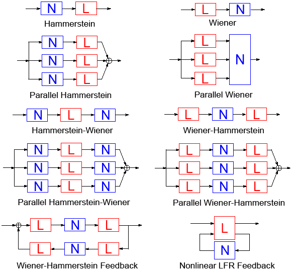
The paper consists mainly of two parts: in the first part (Section II and Section III) we introduce a formal linearization framework (choice of the excitation, choice of the linearization, study of the linearization properties for cascaded and closed loop nonlinear systems). Next, in Section IV, we use these results to obtain structural information by applying these concepts to a number of general block-oriented model structures.
II Class of excitation signals
The retrieval of structural information starts from a set of linear approximations of the nonlinear system, collected at different set points as specified later in this paper. A linear approximation depends strongly on the nature of the excitation signals, and the approximation criterion that is used. In this section we discuss three classes of excitation signals. We start with the class of Gaussian excitation signals, extended with random phase multisines (Schoukens et al., 2009). For these signals it will be illustrated in Section III that it is difficult to express the linearization of the complete complex block-oriented systems (cascaded or closed loop block-oriented systems) as a function of the linearization of the sub-systems. To get around this problem, we will consider excitation signals that become infinitely small, leading to the class of bounded excitations: signals for which the standard deviation or the maximum amplitude is bounded by , and next we will analyze the linearization results for . The latter will allow us to include also the classical small signal network analysis results in the study. For these two classes of signals, it will become possible to write the linearization of the full system as a function of the linearization of the sub-systems. For simplicity, we will define all the signals in the discrete time domain. It is possible to extend the results to the continuous time domain.
II-A Class of Riemann equivalent Gaussian excitations
A first class of excitation signals that we consider is the class of Gaussian excitation signals, extended with random phase multisines. These signals will be applied to the nonlinear system, operating around its setpoint. To do so, a DC offset value will be added later to the excitations, in the remainder of this section, we do not consider this DC-offset.
Definition 1.
Random phase multisines
Consider a power spectrum , that is piece-wise continuous, with a finite number of discontinuities. A random phase multisine is given by
| (1) |
for and with . The Fourier coefficients are either zero (the harmonic is not excited) or their amplitude equals . The amplitude function is set by the desired power spectrum :
The phases are i.i.d. such that .
Remark: The most popular choice for the random phases is to select them uniformly distributed on , resulting in . However, also a discrete distribution can be used, for example a binary distribution .
Random phase multisines are asymptotically normally distributed (), and belong to a more general class of Riemann equivalent Gaussian excitation signals (Schoukens et al., 2009). Evidently, these include also the non-periodic random excitations.
Definition 2.
Class of Riemann equivalent excitation signals
Consider a power spectrum , that is piece-wise continuous, with a finite number of discontinuities.
A random signal belongs to the equivalence class if:
i) It is a zero mean Gaussian noise excitation with power spectrum
or
ii) It is a zero mean random phase multisine s.t.
with , and .
It is known (Pintelon and Schoukens, 2012; Schoukens et al., 2009) that exciting a system by any signal within a fixed class of Riemann equivalent signals , leads asymptotically ( to the same best linear approximation.
II-B Class of excitations
Despite the fact that the class of excitation signals is very useful to deal with nonlinear systems in real life measurements, it has some drawbacks in structure detection. As mentioned before, we will illustrate in the next section that they are not easy to deal with in the context of the theoretical study that is conducted here. It will turn out that for the structure detection purpose, it is more convenient to consider signals that become infinitely small. For such excitation signals, the linearization of a cascade equals the cascade of the linearization which will be the key to address the structure analysis problem. It is clear that such a signal can not be used in practice, but it will allow us to formalize the methods that are proposed in this paper. Turning these results into a guidelines for the practicing engineer remains out of the scope of this paper.
In this section we focus on the signal , combined with a DC-offset :
The excitation operates around a setpoint , and becomes very (infinitesimally) small as specified below. This allows us to isolate the linear term of a system operating around a fixed setpoint . The precise description of is given in the next definition.
Definition 3.
Class of excitations
The signal , , belongs to the class of excitations , if it belongs to the class of Riemann equivalent excitation signals (Definition 2), and
excitations are (asymptotically) normally distributed signals with a limited variance. In this paper results are given for converging towards zero.
II-C Small signal analysis
The idea of linearizing a nonlinear system around a given setpoint is intensively used during the design and analysis of complex electronic circuits. Popular general purpose simulation packages like SPICE (Nagels and Pederson, 1973) offer small signal analysis options based upon a linearization of the original system equations as used above. A theoretic foundation for this approach can be found in the paper of Desoer and Wong (1968), where it is shown that the solution of the linearized nonlinear system equations comes arbitrarily close to the small signal solution of the original nonlinear equations for excitations with an amplitude that tends to zero. The major condition to proof this result is that the second derivative of the nonlinear functions exist. The approach that is developed in this paper can directly be applied on the results of a small signal analysis. To include these in the formal analysis that we present here, we need to add another class of small excitation signals.
Definition 4.
Class of excitations
A signal , , belongs to the class of excitations , if
Remarks:
i) We did not specify the power spectrum of in the previous definition. The small signal analysis can be made using either a stepped sine excitation, or using one of the other popular broadband excitations. While this choice can have a strong impact on the practical aspects of the simulation (for example the computation time), it will not affect the theoretical results.
ii) Also the amplitude distribution is not specified, is not requested to be Gaussian distributed as it was the case for the class for excitations.
iii) It might seem more logic to select as the amplitude bound in the definition. However, in order to simplify the presentation of the theorems later in this paper, we prefer to use the same upper bound in the definitions of and in order to simplify the formulations of the theorems that follow later in this paper.
III Linearization of nonlinear systems
In this section we will first formally introduce the linearizations that we consider in this paper. Next we give a brief discussion of the related properties.
III-A Definitions of the linear approximations
We focus first on Riemann equivalent excitations, as specified in Definition 2. The best linear approximation with respect to a given class of random excitations is given by:
Definition 5.
Best linear approximation around a setpoint
Consider an excitation . The best linear approximation around a given setpoint is then given in the time domain by:
| (2) |
with and or (Enqvist and Ljung, 2005; Enqvist, 2005). In the frequency domain:
| (3) |
(Pintelon and Schoukens, 2012).
Remarks:
i) The expected value is the ensemble average over multiple realizations of the random excitation .
ii) In these expressions, is the impulse response of the best linear approximation, while is the frequency response function (FRF) of the best linear approximation. The dependency of on the setpoint is not explicitely reflected in the notation in order to keep the expressions simple.
iii) The best linear approximation is equal to the describing function for Gaussian noise excitations, as discussed in the book of Gelb and Vander Velde (1968) provided that these excitations operate around the same setpoint and have a Riemann equivalent power spectrum.
The output of a nonlinear system at frequency can always be written as (Pintelon and Schoukens, 2012):
| (4) |
The first term describes that part of the output that is coherent with the input, the second part describes the non-coherent part.
Definition 6.
Local linear model , and
Consider the best linear approximation obtained for a random excitation , and . Define:
| (5) |
and
| (6) |
Consider the best linear approximation obtained for a (random) signal . Then we define:
| (7) |
and
| (8) |
It is possible to extend the definition of to deterministic signals. This is discussed and formalized in Makila and Partington (2003), using the Fr�jet derivative. We refer the reader to this reference for more detailed information. One of the major differences is that the Fr�jet derivative requires the function to be differentiable, while this is not the case for the linearization.
III-B Discussions of the properties of the linearizations
It would be a natural choice to use the best linear approximation to retrieve structural information about the block-oriented models because it is a very convenient tool to use in practice, and many successful applications are reported (Pintelon and Schoukens, 2012). However, it turns out that a straight forward application of this idea to structure determination fails for a number of reasons:
i) The best linear approximation of a cascaded nonlinear systems is not equal to the product of the best linear approximations of the individual subsystems (Dobrowiecki and Schoukens, 2009).
ii) The best linear approximation of a closed loop system is not equal to the closed loop calculated from the best linear approximation.
iii) For non Gaussian excitations, the best linear approximation of a static nonlinear system can become dynamic as is illustrated in Enqvist (2005). It is clear that this would disturb an analysis that is based on the linearized dynamics of the nonlinear system.
For those reasons we have to use a more restricted approach that will be offered by the linearization or the small signal analysis (called here linearization). It the following sections, it will be shown that these linearizations have the properties that are needed to come to a simple analysis.
III-B1 Linearization of a static nonlinear system
In this section we discuss the and linearization of a static nonlinear system . First, we formalize the assumptions on the static nonlinear system. Next, we present the linearization properties. We use the following notations:
- the left and right limit of in is respectively and
- the left and right derivative of with respect to in is and .
Assumption Consider a static nonlinear system . In the setpoint , we make one of the following three sets assumptions:
i) is discontinuous in with , and . The left and right derivatives with respect to can be different and are respectively: and .
ii) is continuous in with . The left and right derivative with respect to are different and are respectively: and .
iii) is continuous and differentiable in with and derivative .
Theorem 7.
and linearization of static nonlinear systems
Consider a static nonlinear system around the setpoint , excited by , with or . Write the output as with . Then the following properties hold for respectively the and linearization of around :
1) If Assumption III-B1-i is valid: the and linearization do not exist, they become infinite.
2) If Assumption III-B1-ii is valid: The linearization does not exist. The linearization exist and is the mean of the left and right derivative: . The output can be written as with and a finite constant. The distribution of the output differs from the normal distribution.
3) If Assumption III-B1-iii is valid: the and linearizations (5) and (7) exist and are equal to each other: . The output can be written as: with
, and a finite constant. The output is (asymptotically) normally distributed for and , if .
Proof: See Appendix.
Remark 1: The linearization does not exist in case 2 of the Theorem. The reason for that is that in a small signal analysis (), the distribution of the excitation is not specified, while the result of the linear approximation depends on it (See Appendix 1).
Remark 2: The result of this theorem can be extended to the cascade of two static nonlinear systems :
a) The linearization of is given by the product of the linearizations of and , provided that meets Assumption III-B1-iii. This requirement is needed in order to guarantee a Gaussian input for the second nonlinearity. The properties of the linearization will then be set by what assumption is valid for .
b) The linearization of is given by the product of the linearizations of and , provided that and meet Assumption III-B1-iii. This requirement is needed in order to guarantee that both linearizations exist.
Remark 3: The results of this theorem can directly be extended to a static nonlinearity that is sandwiched between two stable systems . In that case the linearizations are given by the convolution of the impulse responses multiplied with the linearization of the static nonlinearity as described in the previous theorem.
III-B2 Linearization of cascaded systems
As discussed before, the best linear approximation of the cascade of two nonlinear systems is not equal to the product of the best linear approximations (Dobrowiecki and Schoukens, 2009). However, the same does not hold true for the and linearization, as shown by the following theorem.
Theorem 8.
and linearization of a cascaded single branch system
Consider the cascaded system in Figure 2, excited around the setpoint by or , where indicates the amplitude constraint of the excitation. Assume that:
- the linear systems are stable,
First assume that Assumption III-B1-iii holds for , while meets Assumption III-B1-ii. Then, the linearization of the cascaded system does not exist. The linearization of the cascaded system is given by the product of the linearizations and around their respective operating points, multiplied with the transfer function . The difference is an .
Next assume that both meet Assumption III-B1-iii. Then the linearization and linearization exist and are equal to each other. The difference is an , and the output is Gaussian distributed for Gaussian excitations.
The proof follows immediately from Theorem 7 and the remarks following that theorem.
III-B3 Linearization of nonlinear feedback systems
In this paper, we define a nonlinear feedback system as a closed loop system with at least one static nonlinearity in the loop. We will show in the next theorem that the or linearization of a nonlinear feedback system is obtained by replacing the static nonlinearity by its or linearization (Assumption III-B1-iii should be met). Without loss of generality, we consider here a feedback loop with a linear system in the feed-forward branch, and a single branch feedback that operates around its setpoint . The Assumption III-B1-iii is needed for the static nonlinear blocks, to obtain a continuous and differentiable feedback branch.
Theorem 9.
or linearization of a nonlinear feedback system
Consider a (dynamic) nonlinear system , that is continuous and differentiable around its setpoint (Assumption III-B1 iii). The nonlinear system is captured in the feedback of a closed loop system:
The closed loop is assumed to be stable on the considered input domain that is set by the reference signal , with or . The value is the response of the nonlinear system to . The or linearization of the nonlinear feedback system is then given by:
are the transfer functions of the linear systems or .
Proof: see Appendix 2.
Remark: This result can be directly generalized to a closed loop system with a nonlinear feed-forward and nonlinear feedback branch.
III-B4 Discussion
The previous theorems show that we can replace the nonlinear sub-systems by their or linearizations in cascaded systems with internal nonlinear feedback loops, provided that the nonlinear sub-systems are continuous and differentiable in their respective setpoints (Assumption (III-B1)-iii). It is important to realize that the linearization depends upon the setpoint of the excitation, or more generally speaking, the biasing of the system or circuit. By varying the biasing, we can vary the linearizations of the sub-systems, resulting in a varying or linearization of the overall nonlinear system. In the next section we will show that these variations provide information about candidate block-oriented models that can and cannot be used to approximate the nonlinear system.
IV Structure discrimination of block-oriented models
The main idea to retrieve structural information of a (block-oriented) nonlinear system is to measure and model the or linearization at a number of setpoints or bias settings, using linear system identification tools in the time- (Ljung, 1999, S�derstr�m and Stoica, 1989) or in the frequency domain (Pintelon and Schoukens, 2012).
A two step procedure is proposed. First, we verify if the poles/zeros of the linearized model vary with a changing setpoint. Next, we compare the observed behavior with that of considered candidate model structures. This hopefully allows many candidate block-oriented models to be excluded.
The reader should be well aware that the converse is not true: passing the linearization test is not a sufficient condition to be sure that the candidate structure is able to model the nonlinear systems behavior.
Three different situations are considered when evaluating the results for different setpoints: i) all poles (zeros) remain fixed; ii) all poles (zeros) vary; iii) some of the poles (zeros) vary with a changing setpoint. This leads to 9 possible combinations, and for each of these we will check if we can propose candidate model structures within the classes of models that are considered in this paper. The discussion will be structured along a growing complexity of the candidate model structures.
There are a number of possibilities to change the setpoint of a system. The first one is to apply the small excitation signals around a given DC-level as discussed before. In that case we have to assume that the DC-gain of all the linear dynamic systems is different from zero, so that a setpoint change affects for sure all branches of the system. An alternative possibility for some systems is to change the setpoints of the nonlinearities by varying the biasing of the system using an external control signal. It is clear that also this possibility can be used to create the varying working conditions that are needed to make the linearization analysis. This is formalized in the following assumption:
Assumption Setpoint changes
Consider a nonlinear block-oriented system containing the static nonlinear functions , , operating around the setpoints respectively. It is assumed that all the setpoints can be changed by external interactions.
In the rest of this paper, we will not deal with the dynamics of the setpoint changes. The analysis is made under steady state conditions for the setpoint: the setpoint is a fixed level, and after each change of setpoint we wait till all transients in the system due to the setpoint change become negligible.
IV-A Single branch systems
In a single branch system, we consider the cascade of linear dynamic systems and static nonlinear systems. Well known members of this class are shown in Figure 1: the Wiener, the Hammerstein, the Wiener-Hammerstein, and the Hammerstein-Wiener system. It is obvious that the cascade of two single branch models results in a new single branch model. In Wills and Ninness (2012), more complex single branch models consisting of cascades of Hammerstein systems are considered.
From Theorem 8 it follows that the or linearization of the cascade is proportional to the product of the transfer functions of all linear dynamic blocks. The gain is set by the product of the linearizations of the static nonlinearities . This leads directly to the following theorem:
Theorem 10.
Consider a single branch model, consisting of a cascade of linear dynamic systems and static nonlinear systems . Assume that the systems meet Assumptions III-B1-iii and IV. The poles and zeros of the or linearization do not depend on the setpoint, and the output of the system is (asymptotically) normally distributed for Gaussian excitations.
Proof: From Theorem 8, it follows that
| (9) |
with
| (10) |
where is the linearization of the static nonlinear system around its setpoint . From (9), it follows immediately that the dynamics of the linearization do not vary with the setpoint, and hence the poles and zeros do not move.
Discussion: From this theorem it follows immediately that a single branch structure can not be used to model nonlinear systems that have linearized dynamics that change with the setpoint: a single branch model will not be able to capture the variations of the poles or zeros that are observed during the linearization test.
This result shows also the very limited capability of these models to describe general nonlinear systems. The transfer function of the linearized single branch model will not change dynamics for different setpoints, only a real scaling factor will vary.
IV-B Feed-Forward parallel systems
In this section we consider single branch systems, put in parallel to each other, like the parallel Wiener-Hammerstein system in Figure 1. In Palm (1979), it is shown that feed-forward parallel Wiener-Hammerstein models are a very flexible models. For that reason we include them in this study.
From Theorem 10, it follows that the precise structure of the individual branches is not important, since the linearization for all these systems can be written in terms of if Assumption III-B1-iii is met. However, in order to make statements about the pole/zero movements when we combine different branches, we will assume that there are no common poles or zeros between the different branches. We also will assume that the nonlinearities differ sufficiently from each other in order to avoid problems with linear dependencies of the linearizations.
The parallel structure will be linearized around a series of setpoints and this will result in varying gains (10) for branch at setpoint . Use these gains as entries for the matrix
| (11) |
Assumption Different branches
Consider a parallel structure with parallel branches. All the nonlinearities in a branch meet Assumption III-B1-iii.
Consider the combined dynamics of the branch, being the product of the transfer functions of the linear systems in that branch. The systems and , belonging to different branches , they have no common poles or zeros.
The matrix (11) is of full rank.
Theorem 11.
The or linearization of a feed-forward parallel system with n branches is given by
| (12) |
Proof: The first result (12) follows immediately from Theorem 10. The second claim follows directly by replacing
in (12), with respectively the numerator and denominator of the transfer function, giving:
| (13) |
The rational form in (13) has fixed poles and moving zeros for varying setpoints.
Discussion:
1) Putting a number of branches in parallel increases the flexibility of the model: the model allows to track changing dynamics by moving the zeros as a function of the setpoint. However, it is still not possible to move the poles. It will be necessary to create a closed loop nonlinear model to add that flexibility as will be shown in the next section.
2) The complexity of the feed-forward parallel model is controlled by the prior unknown number of branches. An estimate can be obtained, in a preprocessing step, by stacking the measured frequency response functions of the linearizations, around the setpoints in a matrix:
Under some regularity conditions, the rank of this matrix is equal to the number of branches , provided that (Schoukens et al., 2013; Schoukens et al., 2015).
IV-C Feed-forward feedback parallel systems
Although nonlinear feedback systems can be approximated in a restricted input domain by an open loop model (Boyd and Chua, 1985), the class of systems allows for a much richer and more complex behavior than the open loop system class. In this section we consider systems that consist of a parallel feed-forward and a parallel feedback path. In its most simple form, either the feed-forward or the feedback system can be a linear dynamic system or a static nonlinear system. The structure of this system will be characterized by:
- the number of branches in the feed forward ( and the feedback (,
- the total number of branches with a static nonlinearity ,
- the total numbers of poles and zeros with for example the number of poles in the feed-forward and the number of zeros in the feedback.
For these systems, the following theorem holds:
Theorem 12.
Under Assumption III-B1-iii and IV, the or linearization of a feed-forward feedback parallel system is given by
| (14) |
with respectively the linear dynamics of the feed-forward or feedback branch. Under Assumption IV-B, and if (at least one nonlinearity in the system), the following results hold when the setpoint is changed:
- •
All the zeros are fixed if and only if (single branch in the feed-forward)
- •
All the zeros move if and only if and (no poles in the feedback, more than one branch in the feed-forward)
- •
All the poles are fixed if and only if (no feedback)
- •
All the poles move if and only if (feedback present)
- •
All the poles and the zeros are fixed if and only if , and (this is a single branch feed-forward system)
- •
Some zeros are fixed, some zeros move if and only if , (a dynamic feed-forward branch), and . The poles of the feedback will result in fixed zeros.
- •
It is not possible that some poles move and some poles are fixed
- •
It is not possible that no poles move, while some zeros move and some are fixed
Proof: The first result (14) follows immediately from Theorem 10. The second set of claims follows directly by replacing in (14). By filling out the conditions for each of the claims, a rational form is retrieved. The proof follows directly by verifying if the poles and/or zeros depend on .
Discussion:
1) Although a nonlinear feed-forward feedback parallel structure looks very general, it turns out that it misses the flexibility to cover all possible situations. In Table I, an overview is given of all possible pole/zero combinations that can be covered by the parallel feed-forward parallel feedback structure.
| single branch | |||
From this table it is clear that some combinations can not be covered by this structure (). One possibility to create such models is to cascade the feed-forward feedback parallel system with a single branch model that will add fixed poles and zeros to the structure. Some off these lacking combinations can also be created with a linear fraction representation (see Section IV-D) or with other dedicated structures as will be illustrated in Section IV-E.
2) It is not so easy to determine the number of branches in the feed-forward and the feedback path. For a system with a single branch feed-forward (, we have that the rank of the matrix
equals , with the element-wise inverse of . However, for a mixed structure with and , the authors are not aware of methods that link the rank of the matrix to the number of branches in the system.
IV-D LFR-models
Consider the linear fraction representation (LFR) of a nonlinear system (Vanbeylen, 2013) in Figure 3.
The linearization of this system is:
| (15) |
which can be rewritten as
Theorem 13.
- •
If and provided that is not a static system: All zeros are fixed, some poles are fixed, some poles move. The fixed poles are those of , while the fixed zeros are those of and . This covers situation in Table I.
- •
If and provided that is not a static system: All zeros move, some poles are fixed, some poles move. The fixed poles are those of , and . This covers situation in Table I.
Discussion: Also the LFR-structure, as defined in Figure 3, misses the flexibility to cover all possible situations. It is, for example, impossible to create a structure where some of the zeros move, while others remain fixed.
IV-E Checking if a structure fits with the observed movements of poles and zeros
In the previous sections, we studied a number of general block-oriented model structures. By comparing the observed pole/zero variations for different setpoints, we can verify if a candidate model structure is compatible with the available experimental results using linear identification methods only, on the basis of the previous theorems. The reader should be aware that the linearization analysis results only in necessary conditions, it does not guarantee that the actual structure will indeed be suitable to model that nonlinear system. However, on the basis of the linearization results, it become possible to propose dedicated structures that meet these necessary conditions.
As an example, consider the structure in Figure 4, with
Such a structure allows for fixed and moving poles and zeros, where the movement is controlled by one parameter that depends on the nonlinear system and the setpoint of the system. This covers situation in Table I. More flexibility can be created by the structure that is shown in Figure 5.
In that case
which allows the movement of the poles to be decoupled from that of the zeros by properly tuning the nonlinearities . It is clear that both dynamic systems can be split over two sub-systems that can be put on the left and right side of the corresponding nonlinearity, without changing . In that case we have Wiener-Hammerstein systems in both nonlinear branches. It is also possible to add a third linear system to the middle branch, which will increase the flexibility of the pole and zero positions even more.
V Simulation example
In this simulation we give an illustration of the results obtained in this paper. A system with two Wiener systems (S1, S2) in parallel in the feed forward, and a Wiener system (S3) in the feedback is considered. The system is excited with a filtered random noise excitation with a standard deviation of 0.01 and a varying setpoints between 0 and 1 in steps of 0.1. Once the initial transients are vanished, 4096 samples are processed using the output error method (Ljung, 1999).
The transfer function of the linear dynamic part of the three systems is given below:
The delay in is added in order to avoid an algebraic loop in the system, so that it can be easily simulated using recursive calculations.
The three static nonlinearities are respectively:
From Table I, it follows that all poles will move, some zeros will be fixed, and some will be move. It is easy to verify that in this case the fixed zero will be the pole of system . The results for a simulation without disturbing noise are given in Figure 6. From this figure it is clearly visible that all the poles move, while some of the zeros are fixed. These are at the expected position.
Remarks:
i) Although there is no disturbing noise added to the output in the simulation, the results will vary over successive realizations of the input, because the estimated linear approximation will be influenced by the stochastic nonlinearities. Adding noise will not change this picture.
ii) In practice, the choice of the level of the excitation and the varying offset levels will be a critical issue. We advice the reader to cover the input range of interest with the different offsets that are applied. In order to tune the excitation level, the nonparametric nonlinear detection methods that are explained in Pintelon and Schoukens (2012) can be used. The signal should be selected such that the signal-to-noise ratio is as high as possible, while at the same time the observed nonlinear distortion levels should made as small as possible in order to meet the assumptions underlying the theory as good as possible.
iii) By making good user choices for the input signal, it is possible to increase the quality of the best linear approximation estimates (Pintelon and Schoukens, 2012).
iv) Till now, we considered special designed experiments around a number of setpoints to directly identify the local linear models. In Bai (2010), a semi-parametric local linear modeling technique is proposed to identify nonlinear systems. Around each ’working point’ a local ARX model is identified. The local neighbourhood where each of these ARX models is valid is set by a well designed kernel function. The results of this paper can also be applied to the poles and zeros of these local ARX models. This can be an interesting alternative for the dedicated experiments that were proposed before to obtain the linearizations.
VI Conclusions
This paper proposes a set of necessary conditions on the structure of candidate block-oriented models for a nonlinear system. To verify these, the dependency of the poles and zeros of linear approximations on setpoint changes is analyzed. Although it is not possible to propose on the basis of this information a model structure that is guaranteed to include the true system structure (no sufficient conditions), it is possible to rule out candidate structures in an early phase of the identification process. The results are illustrated on a number of popular block-oriented model structures.
Appendix 1: Proof of Theorem 7
We give the proof for , and we will add additional remarks where needed for .
- It is known from the Bussgang theorem, that the best linear approximation of a static nonlinear system, excited with Gaussian noise (), is also a static system, hence the definition (2) reduces to:
| (17) |
with a constant. The solution of (17) is:
| (18) |
- We have that:
- For , the expected value can be written as the sum of the contributions for and .
This expression reduces to
Observe that
and
From these observations, the proof follows immediately for the different situations:
1) is discontinuous in , hence :
and
A similar argumentation can be used for the linearization: the output remains finite while the input converges to zero.
2) f is continuous (, the derivative does not exist.
In that case we have that within an ,
From this result it turns out that the linearization depends upon the distribution of the excitation. Since the distribution for the class of signals is not specified, it follows that the linearization does not exist. For excitations belonging to we have that:
| (19) |
This proves the first part of the second statement for the linearization.
To prove the second part of the statement consider the difference
| (20) |
It follows immediately that
Since the power of the error term converges to zero with the same rate as that of the linear term , we have that the distribution of will be the convolution of a Gaussian distribution with that of the distribution of , and the latter is not normally distributed. This proves the last claim.
3) is continuous in , and the derivative in exists.
In that case, , and from (19), it follows immediately that
The second part from the claim follows from the observation that the derivative of exist in the operating point . A direct consequence is that the non-Gaussian output contribution (20) converges faster to zero than that of the linear term, and hence the distribution of converges to that of , which is (asymptotically) normal.
For we can consider the linear term of the Taylor expansion which is again given by . Also here the error term will be an .
Appendix 2: Proof of Theorem 9
We give the proof here for , the proof for the linearization is completely similar. Since the nonlinear system is continuous and differentiable (Assumption III-B1-iii), we have that for a stable system, converges to zero when the excitation goes to zero. It then follows immediately from Theorem 7 that the output of the nonlinear system in the feedback loop is given by:
so that we can replace the feedback by its linearization. The proof follows then immediately by replacing the nonlinear system by its linearization .
References
- [Bai (2010)] Bai E.W. (2010). Non-parametric nonlinear system identification: an asymptotic minimum mean squared error estimation. IEEE Trans. on Automatic Control, 55, pp. 1615-1625.
- [Billings and Fakhouri (1982)] Billings, S.A. and S.Y. Fakhouri (1982). Identification of systems containing linear dynamic and static nonlinear elements. Automatica, 18, pp. 15-26.
- [Billings (2013)] Billings, S. A. (2013). Nonlinear system identification : NARMAX methods in the time, frequency, and spatio-temporal domains. John Wiley & Sons Ltd.
- [Bussgan (1952)] Bussgang J.J. (1952). Cross-correlation functions of amplitude-distorted Gaussian signals. Technical Report, 216, MIT Laboratory of Electronics, 1952.
- [Boyd and Chua (1985)] Boyd S. and L.O. Chua (1985). Fading Memory and the Problem of Approximating Nonlinear Operators with Volterra Series. IEEE Trans. on Circuits and Systems, 32, pp. 1150-1161.
- [Desoer and Wong (1968)] Desoer, C.A. and K.K. Wong (1968). Small-Signal Behavior of Nonlinear Lumped Networks. Proc. of the IEEE, 61(1), pp. 14-22.
- [Dobrowiecki and Schoukens (2006)] Dobrowiecki T. and J. Schoukens (2006). Robustness of the related linear dynamic system estimates in cascaded nonlinear MIMO systems. 23rd IEEE Instrumentation and Measurement Technology Conference, Sorrento, Italy, pp. 117-122.
- [Enqvist and Ljung (2005)] Enqvist M. and L. Ljung (2005). Linear approximations of nonlinear FIR systems for separable input processes. Automatica, 41(3), pp. 459-473.
- [Enqvist (2005b)] Enqvist M. (2005). Linear Models of Nonlinear systems. PhD Thesis No. 985, Institute of technology, Link�ping University, Sweden, 2005.
- [Gelb and Vandervelde (1968)] Gelb, A., and W. E. Vander Velde. Multiple-Input Describing Functions and Nonlinear System Design. McGraw Hill, 1968.
- [Giri and Bai (2010)] Giri, F. and E.W. Bai (Eds.), (2010). Block-oriented Nonlinear System Identification. Springer.
- [Haber and Keviczky (1999)] Haber, R., and Keviczky, L. (1999). Nonlinear System Identification: Input-Output Modeling Approach. Dordrecht: Kluwer Academic Publishers.
- [Hunter and Korenberg (1986)] Hunter I.W. and M.J. Korenberg (1986). The identification of nonlinear biological systems: Wiener and Hammerstein cascade models. Biological Cybernetics, 55, pp. 135-144.
- [Korenberg (1991)] Korenberg M.J. (1991). Parallel cascade identification and kernel estimation for nonlinear systems. Annals of Biomedical Engineering, 19:429–455.
- [Lauwers et al. (2008)] Lauwers L., J. Schoukens, R. Pintelon, M. Enqvist (2008). A nonlinear block structure identification procedure using Frequency Response Function measurements. IEEE Trans. on Instrum. and Meas., 57, pp. 2257-2264, 2008.
- [Ljung (1999)] Ljung, L (1999), System Identification: Theory for the User (second edition). Prentice Hall, Upper Saddle River, New Jersey.
- [Makila and Partington (2003)] M�kil� P.M., and J.R. Partington (2003). On linear models for nonlinear systems. Automatica 39, pp. 1-13.
- [Nagel and Pederson (1973)] Nagel, L. W, and Pederson, D. O. (1973). SPICE (Simulation Program with Integrated Circuit Emphasis), Memorandum No. ERL-M382, University of California, Berkeley, Apr. 1973
- [Palm (1979)] Palm, G. (1979). On representation and approximation of nonlinear systems. Biological Cybern., 34, pp. 49-52, 1979.
- [Pintelon and Schoukens (2012)] Pintelon, R. and J. Schoukens (2012). System Identification. A Frequency Domain Approach. 2nd edition. Wiley - IEEE-press, Piscataway.
- [Schetzen (2006)] Schetzen M. (2006). The Volterra and Wiener Theories of Nonlinear Systems. Wiley and Sons, New York.
- [Schoukens et. al. (2008)] Schoukens J., L. Gomme, W. Van Moer, et al. (2008). Identification of a block-structured nonlinear feedback system, applied to a microwave crystal detector. IEEE Trans. Instrum. and Measurem., 57, pp. 1734-1740.
- [Schoukens et al. (2009)] Schoukens J., J. Lataire, R. Pintelon, and G. Vandersteen (2009). Robustness issues of the equivalent linear representation of a nonlinear system. IEEE Trans. Instrum. Meas., vol. 58, pp. 1737-1745.
- [Schoukens et al. (2013)] Schoukens M., G. Vandersteen, Y. Rolain (2013). An identification algorithm for parallel Wiener-Hammerstein systems. IEEE Decision and Control Conference, CDC 2013, pp. 4907-4912.
- [Schoukens et al. (2013)] Schoukens M., A. Marconato, R. Pintelon, G. Vandersteen, Y. Rolain (2015). Parametric identification of parallel Wiener-Hammerstein systems. Automatica, 51, pp. 111-122.
- [Soderstrom and Stoica (1989)] S�derstr�m, T. and P. Stoica (1989). System Identification. Prentice-Hall, Englewood Cliffs 1989.
- [Vanbeylen (2013)] Vanbeylen L. (2013). Nonlinear LFR block-oriented model: Potential benefits and improved, user-friendly identification method. IEEE Trans. on Instrum. and Meas., 62, pp. 3374–3383, 2013.
- [Westwick and Kearney (2003)] Westwick, D.T. and R.E. Kearney (2003). Identification of Nonlinear Physiological Systems. IEEE-Wiley.
- [Wills and Ninness (2012)] Wills A. and B. Ninness (2012). Generalised Hammerstein-Wiener system estimation and a benchmark application. Control Engineering Practice, 20, pp. 1097-1108.