From Real to Complex: Enhancing Radio-based Activity Recognition Using Complex-Valued CSI
Abstract
Activity recognition is an important component of many pervasive computing applications. Radio-based activity recognition has the advantage that it does not have the privacy concern and the subjects do not have to carry a device on them. Recently, it has been shown channel state information (CSI) can be used for activity recognition in a device-free setting. With the proliferation of wireless devices, it is important to understand how radio frequency interference (RFI) can impact on pervasive computing applications. In this paper, we investigate the impact of RFI on device-free CSI-based location-oriented activity recognition. We present data to show that RFI can have a significant impact on the CSI vectors. In the absence of RFI, different activities give rise to different CSI vectors that can be differentiated visually. However, in the presence of RFI, the CSI vectors become much noisier and activity recognition also becomes harder. Our extensive experiments show that the performance of state-of-the-art classification methods may degrade significantly with RFI. We then propose a number of counter measures to mitigate the impact of RFI and improve the location-oriented activity recognition performance. We are also the first to use complex-valued CSI to improve the performance in the environment with RFI.
Index Terms:
Device-free, activity recognition, sparse representation classification, radio frequency interference , channel state informationI Introduction
††footnotetext: Part of this research work has been published in the proceedings of the 14th International Conference on Information Processing in Sensor Networks (IPSN ’15) [37]. We propose a new device-free activity recognition method using complex-valued Channel State Information (CSI) in Section III in this paper. The discussion regarding the evaluation on complex-valued CSI can be found in Section IVActivity recognition aims to identify what a subject is doing. It is an important component of many pervasive computing applications. For example, the increasing greying population in many countries puts a rising pressure on the health care system. Activity recognition can be used to improve home care for the elderlies. This paper considers the activity recognition problem using radio signals, in the device-free setting, with an emphasis on making activity recognitions robust to radio frequency interference (RFI).
Activity recognition is a well researched topic. In terms of system components, there are three broad approaches to the activity recognition problem: camera-based [19, 7, 54, 4, 16], sensor-based [12, 3, 21, 8, 43, 6, 49] and device-free [36, 29, 35]. Cameras are able to provide high resolution data for activity recognition but privacy is a serious concern. Although there is no privacy concern with the sensor-based approach, it imposes the requirement that a subject has to carry sensors on his body. This is inconvenient and activity recognition fails if the subject forgets to carry the device. We have therefore chosen the device-free approach in this paper.
In the device-free approach to activity recognition, radio devices are placed in the periphery of a monitored area, called the area of interest (AoI). These radio devices send packets to each other regularly and use the received radio signal to obtain information on the radio environment. The key idea is that the radio environment is influenced by the activity taking place in the AoI. The activity recognition problem is to infer the activity from the received radio signal. In general, there are three requirements for device-free activity recognition: informative measurements, capability to deal with environment changes, and robustness to RFI.
Using informative measurements is a pre-requisite for any successful classification problem. Although coarse-grained radio channel measurements, such as radio signal-strength indicators (RSSI), have been successfully used for device-free indoor localisation [50, 40, 38], they are no longer informative for activity recognition. Recent work on device-free activity recognition [36, 29, 35] has therefore used Channel Frequency Response (CFR) or Channel State Information (CSI) for activity recognition. This is also our observation and our proposed solution therefore uses CSI.
A challenge for CSI-based device-free activity recognition is that the CSI of the radio channel is sensitive to changes in the environment due to for example new or moved furniture. This is because the CSI-fingerprint of an activity is affected by multi-path effects of the environment. A CSI-based activity recognition method called E-eyes [36] proposed a semi-supervised approach to address the issue of environmental changes. When the system detects that the CSI-fingerprint for an activity has changed, E-eyes requires the users to label the new CSI-instances manually. A similar approach was used in [24] to deal with the impact of environmental changes on CSI-based localisation.

Another challenge for CSI-based activity recognition is that the CSI is highly influenced by RFI. The number and types of radio devices have proliferated in the last decade. It is hardly possible to find a frequency band that is clean or without RFI. Our observation, which is depicted in Fig. 1, shows that CSI is highly impacted by RFI. The figure shows a CSI without RFI as well as a CSI with RFI in a particular radio channel. The impact of RFI on CSI is conspicuous. This implies that CSI-based activity recognition must be robust to RFI. This is the key topic of this paper.
As a summary of the above discussion, we have drawn a Venn diagram with the three requirements of informative measurements, robustness to environmental changes, and robustness to RFI in Fig. 2. This diagram is used to differentiate our work (indicated by a star) from two other CSI-based activity recognition solutions: E-eyes [36] and Sigg et al. [29]. It shows which solution is able to deal with which requirements. Neither of [36, 29] addresses the impact of RFI on CSI.
In order to enable the robustness of CSI-based location-oriented activity classification, our previous research [37] exploits the SRC approach based on -optimisation. SRC has been shown to be robust to noise. It has also been shown to significantly improve the classification performance in face recognition [41, 27] and acoustic classification [39], outperforming other classification approaches such as support vector machine (SVM) and -nearest neighbours (NN). Our previous research [37] also proposed SRC based method on the amplitudes of CSI vectors (real-valued CSI) to mitigate the influence of RFI and increases the performance of real-valued CSI based activity recognition. In this paper, we propose a new classification method to further enhance the robustness of activity recognition using complex-valued CSI. Location-oriented activity recognition is able to indicate the location information as well as types of activities.
To summarise, the contributions and novelties of this paper are:
- •
We demonstrate by using measurements that CSI is highly impacted by RFI. We show that, while the CSI vectors for different activities in a RFI-free environment are clearly distinguishable even by naked eyes, this is no longer the case for an environment with RFI.
- •
To address the above challenge, we propose a novel complex-valued CSI based classification algorithm for CSI-based location-oriented activity recognition. The algorithm fuses the results from a number of -optimisation according to their signal-to-noise ratios (SNRs). We show that this method can boost recognition accuracy and outperforms NN and other SRC-based methods by up to 10%.
- •
We are also the first to use complex-valued CSI for a SRC-based classification algorithm. Complex valued CSI contains phase information additional to amplitude information. We show this can improve the performance compared with using only real-valued CSI.
- •
We study the impact of channel bandwidth on the accuracy of activity recognition. We use 4 different bandwidths: 5, 10, 15 and 20 MHz, which cover low bandwidth devices (e.g. ZigBee) and high bandwidth devices (e.g. WiFi). We show that our proposed classification algorithm produces good classification accuracy for activities with 20 MHz of bandwidth.
The rest of this paper is organised as follows. Section II presents background materials on CSI and SRC. We then study the impact of RFI on CSI and propose our complex-valued CSI based activity recognition method in Section III. Next, we present evaluation results in Section IV using experimental data collected from an apartment. Section V presents related work. Finally, Section VI concludes the paper.
II Background
II-A Wireless Platform and Channel State Information
We use a platform called Wireless Ad hoc System for Positioning (WASP) [22] for our experiments. The WASP nodes are originally designed for high resolution localisation and use a much wider bandwidth than many off-the-shelf wireless devices. WASP can operate in both 2.4 GHz and 5.8 GHz industrial, scientific and medical (ISM) bands, using a bandwidth of, respectively, 83 MHz and 125 MHz. WASP uses Orthogonal Frequency-Division Multiplexing (OFDM) at the physical layer and time division multiple access (TDMA) at the media access control (MAC) layer. In fact, the physical layer of WASP is implemented by using commercial off-the-shelf IEEE 802.11 radio chips.
OFDM is a multi-carrier modulation technique. At the 5.8 GHz band, the WASP nodes use 320 sub-carriers. Each of these sub-carriers has a different centre frequency. This means the received sub-carriers at two frequencies can experience different amount of phase shifts, giving different frequency response. For a sub-carrier with centre frequency , the complex channel response is related to the transmitted symbol and received symbol by . The complex number captures, respectively, the sub-carrier gain and phase shift. Let denote the centre frequencies of the 320 sub-carriers that WASP nodes use. Then the CSI is a complex vector . More details about CSI can be found in [48]. Our previous research [37] only uses the amplitude (gain) of CSI of each sub-carrier, while in this paper complex-valued CSI is applied, which contains both the amplitude and phase shift, to improve the classification accuracy.
II-B Sparse Representation Classification
Sparse Representation Classification (SRC) is first proposed in [41] for face recognition. It has subsequently been applied to other areas, such as acoustic classification [39] and visual tracking [14]. A key feature of SRC is its use of minimisation to make the classification robust to noise.
We give a brief description of SRC here, the details can be found in [41]. We assume that the classification problem has classes. Class is characterised by the sub-dictionary where () are the feature vectors derived from training data. For classification, the sub-dictionaries are concatenated to form a dictionary . Ideally, a test sample should sit in a subspace spanned by the dictionary, i.e. there exists a coefficient vector such that . However, due to noise, such an cannot be found or is perturbed. Instead, the SRC method solves for the coefficient vector using the following optimisation problem:
| (1) |
where is the noise level. Note that instead of requiring that , the constraint requires only that the vectors and are sufficiently close to each other. The estimated coefficient vector is used for the classification algorithm. Note that the length of is . Let denote the -dimension sub-vector in that corresponds to the sub-dictionary . We calculate the residual for Class . The class that gives the minimum residual is returned as the classification result. It is important to point out that this SRC formulation can be used with real or complex-valued and , and optimisation is also capable of handling complex-valued vectors [32, 31].
SRC has a main superiority: featureless. This provides us an opportunity to build a training set from the CSI measurements rather than exacting feature from them. Moreover, SRC is known to be robust to noise. As our work is to study the performance of activity recognition when RFI is present, we investigate how to explore SRC to boost SNR for improving recognition performance. As far as we know, we are the first to use a SRC classification method on complex numbers.

III Activity Recognition using Complex-valued CSI
This section presents our method to recognise a set of location-oriented activities using CSI in the device-free setting. We first demonstrate that complex-valued CSI is influenced by activities taking place in a room and can be used to identify location-oriented activities. We demonstrate the challenge of CSI based activity recognition when RFI is present. Finally, we present our SRC based classification method which takes RFI into consideration.
III-A CSI contains location-oriented activity information
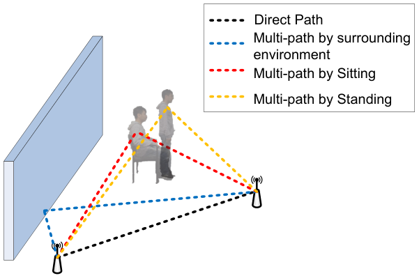
We first present some intuition on why device-free CSI-based location-oriented activity recognition is possible. Fig. 3(a) depicts an indoor environment with two wireless nodes and the multi-paths that the radio propagation may take. It shows that different multi-path effects can be obtained if a person is sitting or standing. Its results in different CSI vectors at the receiver and can be used to identify the activity (normalised CSI amplitude vector shown in Fig. 3(b)). Furthermore, different locations of a monitored person also differentiate multi-paths, which makes location-oriented activity recognition feasible.
In order to demonstrate the feasibility of CSI-based activity recognition, we set up two WASP nodes in an apartment with one living room and one bedroom. The nodes are 5 metres apart with 3 walls in the line-of-sight path between the nodes. The subject is positioned in an AoI between the two nodes but is not in the direct path between the 2 nodes. The subject carry out 4 different activities: sitting, lying, standing, and walking. A WASP node is used as the transmitter and the other as a receiver. The transmitter sends to the receiver at 10 packets per seconds, and it needs a 2.5 milliseconds slot to send a packet. This means only 2.5% of running time is occupied for sending data for activity recognition, which does not occupy bands too much to affect the radio communication of other wireless devices. For each packet received, the receiver uses the WASP interface to obtain the CSI vector and SNR for that packet. It is also important to point out that the data in this experiment are collected in a clean environment without any RFI.
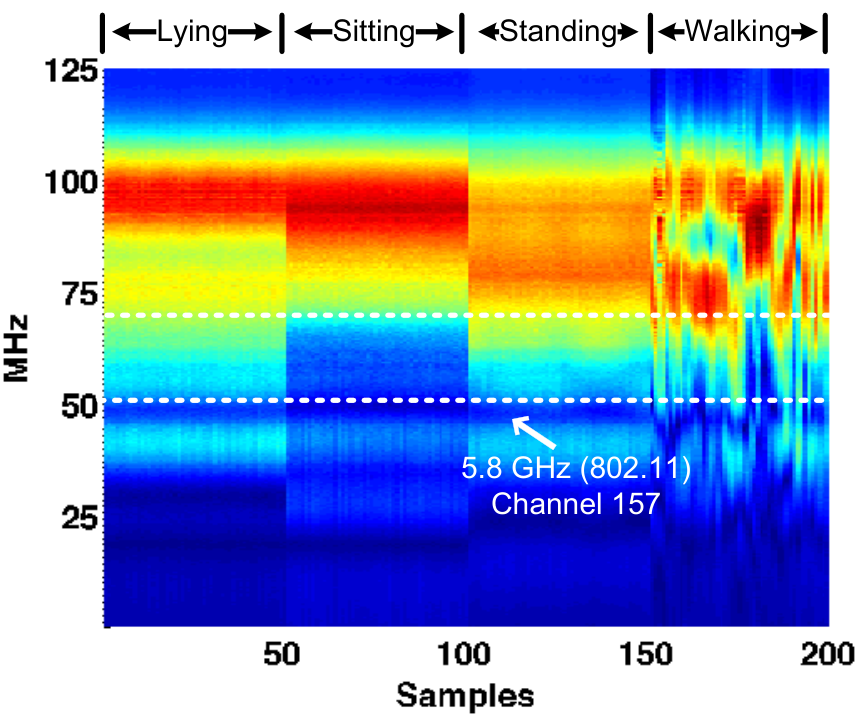
Fig. 5(a) shows the normalised CSI amplitude vectors under the four different activities. The horizontal axis shows the sample number where a sample corresponds to a packet. There are 320 values in the vertical axis which corresponds to the 320 sub-carriers. The magnitude is shown as a heat plot. We have put four blocks of data side-by-side in the figure, which corresponds to the four activities of lying, sitting, standing and walking. It can readily be seen that the four activities have highly distinguishable CSI. This confirms that CSI contains information on activity. Another observation is that the CSI fluctuates a lot when the subject is walking. This is due to different multi-path effects created by the person walking. Fig. 5(a) shows the CSI when a 125 MHz bandwidth is used. We now show that the same observations also apply when we use a 20 MHz channel. The box in Fig. 5(a) is Channel 157 in the 802.11 standards with 20 MHz bandwidth. We have enlarged the CSI in the box and plotted it in Fig. 5(b). It can be seen that the CSI for the four activities are very distinguishable and walking creates more fluctuations in CSI.
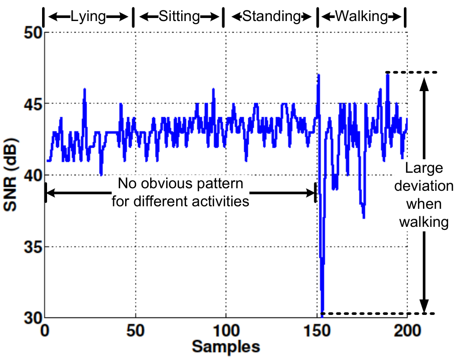
Fig. 5(c) shows the SNR of the corresponding samples (packets). It shows that the SNR has a slightly larger fluctuation when the subject is walking. However, there does not appear to be any noticeable differences in the SNR data series among lying, sitting, and walking. These observations suggest that it may be possible to use SNR to distinguish between walking from the other three activities where the subject is stationary. However, it does not seem to be possible to use SNR to distinguish between the three stationary activities.
Since CSI is sensitive to the multi-path effect, same activity in different locations can have different CSI. Training in each interesting location must be performed for location-orientated activity recognition, and this is a limitation of CSI-based finger-printing activity recognition. Fig. 4 demonstrates the different CSI amplitudes as a result of the same activity “standing” in two locations. This fact requires additional training for same activity in different locations, but it helps location-orientated activity recognition systems locate activities. [45, 44, 36, 29, 15] also apply a similar strategy, i.e. conducting training in various locations, for improving the performance of radio-based pattern recognition.




III-B Challenges of CSI-based activity recognition
The results above are obtained when the two WASP nodes are in a clean environment without RFI. We conduct another experiment using the same set up but we add a pair of IEEE 802.11a devices that communicates in Channel 157 (a 20 MHz band). Our goal is to understand the impact of RFI on CSI and SNR.
Fig. 5(d) shows the CSI for the four activities when RFI is present in Channel 157. It shows that the CSI in Channel 157 (enclosed by the white rectangle) is fairly noisy but the four activities still have distinguishable CSI outside of Channel 157. This suggests that if wide-band devices are used to obtain the CSI for activity recognition, then we can use the part of CSI with little RFI to identify the activity. However, with ubiquitous use of wireless technologies such as WiFi, Bluetooth, IEEE 802.15.4, etc., it becomes more and more difficult or even impossible to find RFI-free bandwidth, particularly in ISM bands, for radio-based activity recognition systems. We therefore consider the possibility of using CSI in an interfered channel to perform activity recognition.
In order to examine the effect of RFI, we plot the CSI of Channel 157 in Fig. 5(e). It shows that the CSI vectors of different activities are no longer highly distinguishable. We now examine the impact of RFI on SNR. Fig. 5(f) shows the SNR of the four activities when RFI is present in Channel 157. We see that the SNR of all four activities are highly fluctuating. We suggested earlier that it would be possible to tell walking from the static activities using SNR when RFI is absent, however, this does not appear to be feasible once RFI is present.
To further show the challenge with RFI, Fig. 6 shows clusters of complex-valued CSI from the same sub-carrier with or without RFI in complex plane. The red spots represent the CSI samples without RFI affected. To better show the scatter of CSI, we shift the centre to (0,0). In clean environment without RFI, all the samples have high SNR and concentrate in a clear cluster. However, in the environment with RFI, the samples scatter in a much larger area, and less pattern can be explored compared with that in clear environment.
However, if we look closer at the CSI vectors of each activity, we can see that a number of CSI vectors among one activity are almost the same. This recurrence of CSI vectors suggests that we may use a block of CSI vectors for classification instead of individual CSI vectors (see Fig. 5(d) and 5(e) ). However, this classification is going to be challenging because the CSI vectors appear to be fairly noisy. We will propose a few different classification methods in Section III-C3 to address this challenge.
To sum up, it is a challenge to use CSI to perform activity recognition when RFI is present.
III-C Location-Oriented Activity Recognition with RFI
We now describe our proposed complex-valued CSI-based activity recognition in the presence of RFI. The goal of activity recognition is to identify four daily activities: sitting, standing, lying and walking in different rooms, as well as whether the AoI is empty.
III-C1 Data collection
Our method fingerprints the activities using CSI complex vectors. The first procedure is to record the CSI measurements and use a CSI data sanitisation method for building a training set, and use the training set to fingerprint the test data by using our proposed machine learning algorithm.
RFI causes the unexpected change to CSI vectors. There is no existing model for the performance of CSI vector under RFI. Therefore, we need to consider the RFI environment when training the dictionary. In other words, the CSI vectors of one specific activity under different physical or radio environments vary significantly. We have to update training set for a new RFI environment. The method in [36] can be applied for updating the dictionary when RFI is present.
III-C2 CSI Data Sanitisation
We use a CSI data sanitisation method to obtain both CSI amplitude and phase information. A CSI vector with sub-carriers, i.e. . The CSI amplitude vector is the absolute values of each elements. Since the receiver and transmitter do not attempt to synchronise time in OFDM and there is an unknown random phase shift in each CSI vector, a data sanitisation method to calculate the phase information for OFDM is required. We use the data sanitisation method proposed in [24] for calculating this unknown phase shift. The details of this algorithm can be found in [24]. Having CSI phase information, we are ready to calculate CSI vectors. The CSI for -th sub-carrier is a complex number , where is the CSI complex value of -th sub-carrier after sanitisation and . We apply this algorithm to all CSI vectors to remove the unknown phase shift. From now onwards, unless otherwise stated, all CSI vectors are assumed to have been sanitised.
The complex values of CSI will contains both amplitude and phase information. This is extremely important for improving performance in the environments with RFI where limited useful data can be explored. Fig. 7 gives an intuitive explanation of this improvement. Consider the CSI of the same sub-carrier for two different classes. Fig. 7(b) depicts the situation when complex CSI is used, the distance d2 between the two classes is the distance between two complex numbers on the plane. However, if only the CSI amplitudes are used, then we get the situation in Fig. 7(a) where the distance between the two classes is d1. It can be shown that d2d1, which means complex CSI enhances the separation between different classes and therefore giving better classification performance.
III-C3 Classification algorithms
We have seen that RFI causes the CSI vector to be very noisy. In order to deal with RFI, we introduce a window size where consecutive complex-valued CSI vectors are used for classification. One possible method is to stack complex-valued CSI vectors into a long feature vector and use it for classification. However, this will be computationally intensive because the feature vector has a very high dimension. Instead, we will use the one complex-valued CSI vector at a time and investigate different fusion methods.
Let denote the complex-valued CSI vectors in the time window, and be the dictionary. We first solve the following -optimisation problem for :
| (2) |
We now present three different fusion methods which use () in different ways.
The first method is to use decision fusion and will be referred to as -voting. For this method, the algorithm uses each to arrive at a decision class using the standard SRC algorithm described in Section II-B. This method then uses majority voting to arrive at a decision.
The second method is to fuse the vectors by computing their mean: . The mean vector is then use to compute the residuals for each class as in the standard SRC algorithm described in Section II-B. This method returns the class that minimises the residual. Note that this fusion method was proposed by Misra et al. in [18] where they showed that such method could improve the GPS recovery accuracy. We will call this method -sumup.
The method -sumup applies equal weights to all by computing a simple average of them. However, it is possible that some CSI vectors in the window are less affected by noise. This can also be seen from Fig. 5 where the SNR fluctuates. We therefore propose to use SNR of a sample to derive a weighting for that sample. Let denote the SNR of the -th sample in the window. We compute the weighted mean of using:
| (3) |
| (4) |
The mean vector is then use to compute the residuals for each class as in the standard SRC algorithm described in Section II-B. This method returns the class that minimises the residual. We call this method as -weighting.
IV Evaluation

IV-A WASP nodes
We use a pair of WASP nodes in our experimental evaluation. We provided some basic information on WASP nodes in Section II-A. We provide further background information and explain some design choices here.
We choose WASP because it is a software-defined radio and there is an API to obtain CSI. WASP can operate in both 2.4 GHz and 5.8 GHz. We choose to perform our evaluation in 5.8 GHz because this band is less used compared to the 2.4 GHz band. It is therefore easier to find places where RFI is absent across the entire 125 MHz bandwidth that WASP operates in. This allows us to do two things. First, we can experiment in a clean radio frequency (RF) environment and use CSI from the clean environment to establish benchmark for the classification algorithms. Second, this allows us to control the amount of RFI present in our experiments and we can be sure that any RFI present in the environment is added by us. We can therefore study the impact of RFI on activity recognition. Another reason for choosing the 5.8 GHz band is that WASP nodes have a bandwidth of 125 MHz in this band. This allows us to emulate protocols with wider bandwidth, e.g. 80 MHz bandwidth for 802.11ac.
WASP is a low-power wireless platform. The energy cost is 2 W when WASP is receiving beacons, and 2.5 W when transmitting. A pair of WASP nodes only consumes 4.5 W [22]. WASP nodes can be powered by cable, which means the deployment of a pair of WASP nodes for activity recognition only cost no more than 4 kWh per month.
| Wireless Protocol | Bandwidth per Channel | Number of Subcarrier in OFDM |
|---|---|---|
| 2.4 GHz (ZigBee) | 5 MHz | 13 |
| 2.4 GHz (802.11b/g/n) | 20 MHz | 52 |
| 3.6 GHz (802.11y) | 5/ 10/ 20 MHz | 13/ 26/ 52 |
| 4.9 GHz (802.11y) | 20 MHz | 52 |
| 5 GHz (802.11a) | 20 MHz | 52 |
| 5 GHz (802.11n) | 20/ 40 MHz | 52/ 104 |
| 5 GHz (802.11ac) | 20/ 40/ 80 MHz | 52/ 104/ 208 |
IV-B Experiment Setup
The experiment is conducted in an apartment whose floor plan is shown in Fig. 8. The AoI includes one living room (top half of the floor plan) and one bedroom (the room on the right). Two WASP nodes are deployed at the edge of the AoI. One node works as the transmitter and sends a beacons once every 0.1 second. This node is near the left-hand end of the apartment and is marked as transmitter in the floor plan. The other WASP node acts as a receiver and this is where the CSI data is collected. This node is located in the balcony just outside the bedroom. This node is marked as the receiver in the floor plan. The receiver is connected to a computer (labelled as PC in the floor plan) in the bedroom and this computer is the sink for the CSI data. The distance between the transmitter and receiver is about 5 metres.
We consider 8 different location-oriented activity classes: (1) E: empty environment (2) L: lying on the bed in the bedroom (3) SiB: sitting in the bedroom (4) SiL: sitting in the living room (5) StB: standing in the bedroom (6) StL: standing in the living room (7) WB: walking in the bedroom (8) WL: walking in the living room. The location of the activities are marked in the floor plan in Fig. 8. We perform standing and sitting in the same location, because we also want to focus on activity classification without considering different locations to evaluate the efficiency of our method. We also differentiate sitting and standing in different locations for evaluating the location-oriented activity recognition. For each activity class, CSI data is collected for 1 minute, so that no physical environmental changes take place during this time. For a given data set, we have 600 CSI samples for each in-place activity, resulting in CSI samples in total.
We use a computer (PC) and a WiFi router to create RFI in the environment. Their locations are marked in the floor plan in Fig. 8. They use 802.11a protocol, which operates in 5.8 GHz, to communicate in Channel 157 (a 20 MHz channel). The computer communicates with the router using the echo request ping command as fast as possible with the default packet size 7 kilobytes; the router responses the request with echo reply packet containing the exact data of request packet. The average transmission rate will arrive at more than 30 Mbit/s. In order to simulate the RFI that the activity recognition system may actually experience, we place the WiFi router in the middle of the apartment, which is a natural location that people will use in order to provide WiFi coverage to their apartment. The distance between the WiFi router and the receiver is about 4 metres, but in one experiment, the router is moved to different locations to create different amount of RFI at the receiver. The distance between the PC and the receiver is about 1.5 metres.
IV-C Evaluation methodology and metrics
We apply 10-fold cross validation to each data set to evaluate our proposed method. The results from the 10 folds are averaged to obtain the final result. We use both the probability of true detection and confusion matrix to present our results.
We have two primary data sets. One data set is collected under clean environment while the other is collected when there is RFI in Channel 157. We use these data sets to investigate the effect of bandwidth on location-oriented activity recognition. In particular, we investigate what happens if we use a bandwidth of 5 MHz, 10 MHz, 15 MHz, 20 MHz, 40 MHz, 80 MHz and 125 MHz. Let us assume that we use a bandwidth window size MHz where is one of 5, 10, 15, 20, 40, 80 or 125. Recalling that WASP nodes have a bandwidth of 125 MHz. We first select the first MHz of the 125 MHz-band and use the sub-carriers in the MHz to perform classification. We then shift the bandwidth window by 5 MHz. If a complete MHz can be found in the data, we perform another calculations. We iterate until the whole 125 MHz is covered. We will refer to the results obtained by sliding bandwidth window over the 125 MHz band as “whole bandwidth without RFI” and “whole bandwidth with RFI”.
Instead of using the whole 125 MHz in the primary data sets. We also created two secondary data sets, from the with and without RFI cases, which include over those sub-carriers in Channel 157. These secondary data sets span a bandwidth of 20 MHz. Note that, when interference sources exist, all sub-carriers in the secondary data sets are with RFI while only some of the sub-carriers in the primary data sets are with RFI. By using the secondary data sets, we investigate what happens when we use a bandwidth window of 5 MHz, 10 MHz, 15 MHz, 20 MHz. The methodology of shifting the bandwidth window is the same as that for primary data sets. We will refer to the results obtained from the secondary data sets as “Channel 157 without RFI” and “Channel 157 with RFI”.
Our classification algorithm uses a window size of consecutive CSI samples for classification, as discussed in Section II-B. We will also vary this window size in our investigation.
We consider the following 4 classification algorithms: NN with majority voting (NN-), - , - and -. In order to demonstrate the improvement in using a window size , we sometimes also show the result of using one CSI sample or a window size of 1; we will use “NN-” and “-” to denote the algorithms that use a . The default SRC algorithms in this section is complex-valued unless we state otherwise. We also use complex-valued NN for comparison.
IV-D Effect of Window Size
In this section, we study the impact of window size on activity recognition performance. We use from 1 to 10, which correspond to a time of 0.1 s and 1 s, because the transmitter sends beacons at a frequency of 10 Hz. We will show that window size can improve accuracy but this is at the expense of decreasing the temporal resolution of activity recognition. We will use both primary data sets (“whole bandwidth without RFI” and “whole bandwidth with RFI”) and both secondary data sets (“Channel 157 without RFI” and “Channel 157 with RFI”) in this study. We assume a bandwidth window size , which is the bandwidth of one 5.8 GHz 802.11 channel. Fig. 9 shows performance in different window size using different data fusion methods.
First, we discuss the performance of using “whole bandwidth without RFI”. Fig. 9(a) shows the probability of true detection of the 4 different algorithms. When there is no RFI and with a 20 MHz bandwidth window size, a window size of 1 can already achieve an accuracy of approximately 90% for all four classification algorithms. The accuracy gradually increases to 95% when the window size is increased to 10. The results are similar if we use “Channel 157 without RFI”, as shown in Fig. 9(c). The algorithms - and - show similar performance but are slightly better than NN and -. This shows that, without RFI, very good classification accuracy can be obtained.
As we discussed earlier, the challenge is to perform classification when there is RFI. Fig. 9(b) shows the probability of true detection for the data set “whole bandwidth with RFI”. It shows that the performance increases with larger window size. Among the four algorithms used, -based algorithms outperform NN and the best performing algorithms are - and -. If we compare the classification accuracy between without and with RFI in Fig. 9(a) and 9(b), we see a significant drop in accuracy when RFI is present especially when the window size is small. For example, for , accuracy decreases from 85% to 76% because of RFI. We now turn to the data set “Channel 157 with RFI” whose results shown in Fig. 9(d). Again,the accuracy increases when the window size is increased, and both - and - perform the best. The most telling observation is that, for , the classification accuracy is merely 63% but if is used, an accuracy of almost 85% can be obtained. This shows that window size can have a significant effect on performance when RFI is present.
We now present the confusion matrices for location-oriented activity recognition using our proposed -. Fig. 10(a) shows the confusion matrix for “Channel 157 without RFI” with a window size of 5 (0.5 second). It shows that perfect accuracy is achieved with 5 activities. The accuracy for static activities is extremely high. The accuracy for the two walking activities are also very good. We now present the confusion matrix for “Channel 157 with RFI” with a window size of 0.1 second and 0.5 second, in respectively, Fig. 10(b) and 10(c). It can be seen that a big window size has significantly improved classification accuracy of many activities. In the following sections, we will use a window size (0.5 second) by default.
IV-E Effect of the Bandwidth Window Size
In this section, we discuss the influence of the bandwidth window size on the location-oriented activity recognition performance. This study takes advantage of the available wide bandwidth from WASP nodes to simulate different kinds of protocols shown in Table I.
The result of using different bandwidth window size for data set “whole bandwidth without RFI” is shown in Fig. 11(a). As expected, increasing gives a better classification accuracy. In particular, - achieves an accuracy of 70%, 90% and 95% when using a bandwidth window of 5 MHz, 20 MHz and 125 MHz respectively. Similar trend is also observed for the data set “Channel 157 without RFI” (shown in Fig. 11(b)). The algorithms -, -, - and NN- show similar performance.
Fig. 11(c) shows the probability of true detection for the data set “whole bandwidth with RFI”. It shows the performance increases when the bigger bandwidth window size increases. Comparing four algorithms using window size 5, - and - perform the best, which outperform - and NN-. When looking at the data set “Channel 157 with RFI” (shown in Fig. 11(d)), the accuracy decreases significantly, especially when the bandwidth window sizes are 5 MHz and 10 MHz whose accuracy decreases from 72% and 88% to 50% and 70% using - compared with the data set “Channel 157 without RFI”. The performance of - and - is close, but they show their superiority over - and NN-, for example, the accuracy of - and - is 5% better than - and NN- when the bandwidth window size is 20 MHz. This shows - and - algorithms increase the recognition performance when there is RFI.
Fig. 10(d), Fig. 10(e), Fig. 10(f) and Fig. 10(c) illustrate the confusion matrix using - with the bandwidth window size 5 MHz, 10 MHz, 15 MHz and 20 MHz respectively in the data set “Channel 157 with RFI”. It shows that the using larger bandwidth window size helps increase the accuracy and robustness to RFI. When the bandwidth window size is 20 MHz, 2 static activities have perfect accuracy, 2 static activities have accuracy more than 90%, the other 2 static activities have accuracy more than 85%, and “walking in bedroom” has the accuracy more than 70%.
IV-F Effect of Different Distances Between the Router and Receiver
In order to evaluate the impact of the amount of interference on classification. We vary the distance between one interferer (the WiFi router in the floor plan in Fig. 8) and the WASP receiver. We consider 4 cases: no interference (NONE), interferer just next to the the receiver (0mR), 0.5 metre away from the receiver (0.5mR), and 1 metre away form the receiver (1mR). The classification uses only Channel 157. The computer also communicates with the router using the echo request ping command as fast as possible.
Fig. 12 shows the influence of receiver-interferer distance on the probability of true detection. It shows that for 0mR, the accuracy can drop by more than 10%. However, by using a window size , - has an accuracy about 60%. Note that there is not much difference between the 0.5mR and 1mR cases. Also, there is only a slight drop in performance for the algorithms between NONE and 0.5mR cases. This shows that if an interferer is not present within 0.5m of the receiver, then the activity recognition accuracy is still high.
IV-G Effect of Different traffic Between Interference Source and Receiver
In this section, we study the effect of traffic sending rates on the classification performance. We keep one interference source (the WiFi router in the floor plan in Fig. 8) next to the receiver and adjust the ping rates of the interferer.
The ping rate is set to “as fast as possible” (average transmission rate more than 30 Mbit/s ), 500 packets per second (transmission rate 28 Mbit/s), 200 packets per second(transmission rate 11.2 Mbit/s), 100 packets per second (transmission rate 5.6 Mbit/s) and 10 packets per second (transmission rate 0.56 Mbit/s). These settings roughly correspond to the bit rates of watching online videos with frame rates 1080p, 480p and 360p, which give rise to bit rates of 8 Mbit/s, 5 Mbit/s and 1 Mbit/s respectively.
Fig. 13 shows the classification performance under different transmission rates. Our proposed - method reaches 80% accuracy when transmission rate is 28 Mbit/s, which means it is robust to the transmission rate 28 Mbit/s. In contrast, the accuracy of both - and NN- algorithm is no more than 70%. This means our proposed - is more robust to RFI than the other methods. Moreover, - achieves an accuracy of 85% when the transmission rate is 11.2 Mbit/s. The accuracy stays almost the same for lower transmission rates.
| Feature | Equation |
|---|---|
| Standard Deviation | |
| Peak | |
| Head Size | |
| 3rd Order Central moment |
IV-H SNR based Walking Detection Discussion
In Section III, we discuss the possibility of using SNR to differentiate walking from non-walking, i.e. a detection or binary classification problem. We see from Fig. 5(c) that, when RFI is absent, this is probably feasible because walking gives rise to highly fluctuating RSS while non-walking does not. However, in the presence of RFI, the distinction between walking and non-walking is not so conspicuous, as seen in Fig. 5(f). In this section, we want to investigate what classification performance we can get if we use SNR for walking detection. This study is also motivated by the fact that many device-free localisation methods [55, 9, 56] use SNR as a feature to find the location of the person in AoI.
The detection problem is to detect whether the person is walking. This covers the classes of WL and WB instead of walking detection with location information. A commonly used feature for device-free localisation is the variance of the SNR, which is used in for example [55]. However, in order to minimise the possibility that walking detection fails due to poor choice of features, we have chosen to use 4 different features listed in Table II: Standard Deviation, Peak, Head Size, and 3rd Order Central moment where is SNR vectors and is the mean of SNR values in a vector. For training, we use a logistic regression model.
The alternative to using SNR for walking detection is to use CSI with classifier. We will compare these two methods. The comparison uses 10-fold cross validation and measurements from Channel 157. We consider two data sets, “Channel 157 without RFI” and “Channel 157 with RFI”. Also, for both data sets, we use bandwidth window sizes of 5 MHz, 10 MHz and 20 MHz bands.
Since walking detection is binary classification, we use the following metrics:
True Positive Rate (TPR):
False Positive Rate (FPR):
F1 score:
where , , and are the number of true positives, true negatives, false positives, and false negatives respectively.
Table III shows the comparison between detection using SNR and using CSI. Each column illustrates one bandwidth window size in each data set and we highlight the better statistics. A number of observations can be made: (1) In the absence of RFI, detection using SNR has a higher TPR compared to using CSI for a bandwidth window of 5 MHz and 10 MHz; however, for a bandwidth window of 20 MHz, detection using CSI has a higher TPR. (2) In the absence of RFI, it is viable to use either SNR or CSI based detector for walking detection. (3) RFI causes the performance of both detectors to decrease. However, the SNR-based detector has a sharper drop in TPR. (4) Overall, the CSI-based detector is more robust in the presence of RFI.
| Without RFI | With RFI | |||||
|---|---|---|---|---|---|---|
| Bandwidth | 5 MHz | 10 MHz | 20 MHz | 5 MHz | 10 MHz | 20 MHz |
| TPR (SNR) | 0.7059 | 0.8740 | 0.9076 | 0.0924 | 0.1975 | 0.4370 |
| FPR (SNR) | 0.0420 | 0.0187 | 0.0070 | 0.0256 | 0.0490 | 0.0506 |
| F1 score (SNR) | 0.7648 | 0.9052 | 0.9407 | 0.1446 | 0.2885 | 0.5428 |
| TPR (CSI) | 0.4706 | 0.8313 | 0.9913 | 0.3277 | 0.5336 | 0.8393 |
| FPR (CSI) | 0.0056 | 0.112 | 0.0084 | 0.0938 | 0.0574 | 0.0309 |
| F1 score (CSI) | 0.6328 | 0.8314 | 0.9833 | 0.4073 | 0.6256 | 0.8393 |
IV-I Effect on Complex-valued CSI
IV-I1 Effect of Complex-Valued CSI Based Classification Discussion
| L1_weight | L1_sumup | L1_voting | L1_w1 | kNN_voting | kNN_w1 | |
|---|---|---|---|---|---|---|
| Complex | 0.935 | 0.930 | 0.909 | 0.879 | 0.913 | 0.889 |
| Real | 0.928 | 0.929 | 0.888 | 0.856 | 0.912 | 0.885 |
| L1_weight | L1_sumup | L1_voting | L1_w1 | kNN_voting | kNN_w1 | |
|---|---|---|---|---|---|---|
| Complex | 0.851 | 0.854 | 0.770 | 0.612 | 0.760 | 0.603 |
| Real | 0.801 | 0.807 | 0.752 | 0.558 | 0.748 | 0.575 |
In this section, we explore the advantage of complex-valued CSI based classification. As illustrated in Fig. 7, complex-valued CSI can enlarge the separation between classes. To further support this, we use the data from the datasets “Channel 157 without RFI” and “Channel 157 with RFI” and calculate the distances between and within classes. We use the metric, which was introduced to calculate the distance between two classes and tune SVM hyperparameters [30]. The distance is defined as
| (5) |
, where and are samples for two classes, and are the numbers of samples in each class. is the -th sample in Class . The function calculates the Euclidean distance between two vectors. This metric considers distances between two classes as well as the distance within each class. We average distances between each pair of classes to calculate class distance. The longer class distance will help improve the classification performance as a result.
Fig. 14 shows the class distances in the datasets “Channel 157 without RTI” and “Channel 157 with RTI” by using real-valued CSI and complex-valued CSI. Please note the real-valued SRC is used for real-valued CSI based classification. In the dataset “Channel 157 without RTI”, the class distance is 0.203 using real-valued CSI. The class distance rises 31.0% to 0.266 when using complex-valued CSI. The class distance decreases to 0.108 when using real-valued CSI in the dataset “Channel 157 with RTI” due to the existence of RFI. When using the complex-valued, the class distance significantly rises 52.0% to 0.166 when using complex-valued. There are two observations: (1) RFI can reduce the class distance, which results in the reduction of the recognition performance. (2) Complex-valued CSI can increase the class distance significantly, and improve the classification results in return.
We will further confirm this using the true detection rates. Table IV shows the true detection rate in the dataset “Channel 157 without RTI”. It shows the accuracy stays similar without RFI when using complex-valued and real-valued based CSI. When looking at the dataset “Channel 157 with RTI” as shown in Table V, the accuracy improves significantly using complex-valued CSI. When using complex-valued CSI, the true detection rate of - increases from 55.8% to 61.2%. Applying data fusion methods, real-valued CSI based -, - and - can achieve 80.1%, 80.7% and 75.2% respectively. When using complex-valued CSI, their accuracy increases to 85.1%, 85.4% and 77.0%. This shows the complex-valued CSI can help improve recognition performance with RFI. Fig. 10(a), Fig. 10(c), Fig. 10(g) and Fig. 10(h) demonstrate the confusion matrices of these settings, which also confirms the fact that complex-valued CSI achieves better recognition performance. complex-valued CSI can supply phase information additional to amplitude information. When the environment is without RFI, the amplitude information is capable to show clear distinguishable patterns, so the performance stays similar in the dataset “Channel 157 without RTI”. However, the additional phase information is important for the scenario with RFI and help improve the recognition accuracy, where CSI amplitude are not sufficiently informative.
IV-I2 Effect of Sanitised CSI
To show the effect of Sanitised CSI, we also use “Channel 157 without RFI” and “Channel 157 with RFI” datasets and the default window size =0.5 second and bandwidth window =5 MHz. For unsanitised CSI, we directly uses the raw CSI vectors without any processing. Fig. 15 shows the true detection rate using sanitised and unsanitised CSI. In the dataset “Channel 157 without RFI”, the accuracy increases from 90.76% to 93.48%. When introducing RFI in the dataset “Channel 157 with RFI”, the accuracy drops to 73.73% with unsanitised CSI. After sanitising, the accuracy increases to 85.08%. This shows it can significantly improve performance using sanitised CSI.
IV-I3 Effect of Complex-valued SRC
In this section, we discuss the effect of SRC using complex-valued CSI. We are the first to apply complex-valued minimisation for classification tasks. To compare with complex-valued SRC, we combine phase vectors and amplitude vectors into one column as inputs (“Features in Column”) for a real-valued SRC. Figure 16 shows the true detection using in the dataset “Channel 157 with RFI” and “Channel 157 without RFI”. In the dataset “Channel 157 without RFI”, the accuracy slightly increases from 93.17% to 93.48%. With RFI in the dataset “Channel 157 with RFI”, the accuracy decreases to 85.08% using our proposed method, while the true detection rate is only 80.36% using “Features in Column” method.
V Related work
We have already discussed the most related work, i.e. work on using CSI for activity classification, in Section I. In this section, we discuss work in three areas: activity recognition, pattern recognition from radio data and the application of compressed sensing in wireless networks.
V-A Activity recognition
Activity recognition forms the basis of many context aware pervasive computing applications. We can broadly classify activity recognition according to whether they are sensor-based or camera-based. Many sensor-based activity recognition systems have been proposed. Acceleration sensor is one of the most frequently used sensors [12, 3, 21]. This is because miniature acceleration sensors are cheap and readily available, and they can be found on all smartphones. For example, Keally et al. [10] used sensors smartphone as well as sensors wore on wrists, ankles and head to distinguish between walking, cycling, sitting and other activities. Recently, a number of wristbands, that are equipped with acceleration sensor, are available in the market. Products such as Jawbone Up [8] and Xiaomi Mi Band [43] can achieve good activity recognition accuracy but they require the users to wear the devices.
Microphone is another sensor that has been used in activity recognition. Hao et al. [6] present a method to monitor sleep quality using microphone; however, it is not sure whether the same method will function in daily activity recognition in a noisy environment. Yatani and Truong [49] designed a wearable acoustic sensor which can be used to record the sound near the throat of the user, and use the measurements for activity recognition. Again, the issue is that the subject has to wear a sensor.
Cameras are also widely used for activity recognition, localisation and tracking [19, 7, 54, 4, 16, 13, 25]. An advantage of camera sensors is that they free the subjects the need to wear or to remember to wear a device. Another advantage is that they provide very rich data which can be used to distinguish between many different activities. However, the Achilles’ heel of using camera for activity recognition is privacy concern. Also, cameras can only cover a limited area. For monitoring in an apartment, a camera is needed in each room. On the contrary, activity recognition using radio signals can cover a much wider area and can “see” through walls, while cameras cannot. We have therefore chosen to use device-free radio-based activity recognition which does not need subjects to carry a device and has no privacy concerns.
V-B Radio based pattern recognition
The propagation of radio waves in an environment is affected by the objects and people in the environment, through reflection, diffraction, constructive and destructive interference and so on. There is much interest in using the received signal characteristics to infer about the attributes of people and objects in an environment. The received signal characteristics used can be coarse or fine grained.
An example of coarse grained radio signal feature is RSSI which measures the received signal power. RSSI has been successfully used in device-free localisation [40, 55, 9, 56, 38, 46]. This is because a person standing in an area between the transmitter and receiver can attenuate, reflect, scatter the radio waves. These effects create a characteristic pattern in RSSI which can be used to infer the location of people in the environment.
Unfortunately, only limited information on the environment can be inferred from RSSI. There is a growing interest to use fine grained features of radio signals for inference. This is also fuelled by the availability of API to query CSI from WiFi chipsets such as Intel 5300 [5] and Atheros 9390 [23]. CSI has been used for many pattern recognition problems, including localisation [24], human detection [57], activity recognition [36, 29], fine-grained gesture recognition [15] , “lip-read” [33], emotion recognition [53], identity recognition[51, 52, 34]. As mentioned in Section I, our work differs from earlier work on using CSI for activity recognition in that we take RFI into consideration while earlier work did not.
Radio signals have also been used to perform gesture recognition. WiSee designed by Adib et al. [2] and WiVi designed by Pu et al. [20] used software-defined radio to extract the Doppler effect caused by the gesture. In order to reduce energy consumption, Kellogg et al. [11] built AllSee which uses RFID tags and power-harvesting sensors for gesture recognition. However, these work can only recognise dynamic gestures and are not able to detect static activities because they rely on Doppler effect. To further improve the resolution of the radio signal based localisation and gesture recognition, Adib et al. [1] designed WiTrack and obtain time-of-flight from the Frequency Modulated Carrier Wave (FMCW) technology for localisation in 3 dimensions. Witrack has high resolution for localisation (approximately 10 cm), but needs to use a bandwidth of 1.69 GHz. However, we show in this paper as few as 20 MHz of bandwidth can be used to distinguish static activities with good accuracy. Moreover, none of these works designed their systems with RFI, while our work takes RFI into consideration.
V-C Application of Compressed Sensing on Wireless Sensor Networks
Recently, compressed sensing has been applied to wireless sensor networks. SRC proposed by Wright et al. [41] is one of the applications of compressed sensing which helps increase the recognition performance. Wei et al. [39] developed an acoustic classification method on wireless sensor networks by applying SRC to increase the recognition performance and decrease the computation time to meet the requirement of real-time classification. Shen et al. [27, 28] optimised the SRC to boost the face recognition performance in smartphones.
Besides recognition, compressed sensing is also applied to background subtraction [25, 26, 47], data compression for in-situ soil moisture sensing [42], and cross-correlation for acoustic ranging [17] and GPS ranging [18].
Compared with these works, this paper is the first to investigate the feasibility of SRC for radio-based activity recognition. Furthermore, our work also takes advantage of SRC for activity recognition with RFI in present.
VI Conclusion
In this paper, we investigate the performance of radio based device-free location-oriented activity recognition systems under RFI using complex-valued CSI, and propose a novel fusion algorithm based on SRC that can improve the recognition performance of the systems by up to 10% when RFI is present. Our prototype robust location-oriented activity recognition systems require only one pair of nodes for a one-bedroom apartment, which enables easy system set-up and maintenance. Finally, we use an embedded wide band radio device (WASP platform) to emulate and study the recognition performance of popular wireless communication protocols that have different bandwidths under RFI.
References
- [1] F. Adib, Z. Kabelac, D. Katabi, and R. C. Miller. 3D tracking via body radio reflections. In NSDI ’14, Seattle, WA, 2014.
- [2] F. Adib and D. Katabi. See through walls with WiFi! In SIGCOMM ’13, pages 75–86, New York, NY, USA, 2013. ACM.
- [3] L. Bao and S. S. Intille. Activity recognition from user-annotated acceleration data. In Pervasive computing, pages 1–17. Springer, 2004.
- [4] I. Cohen and H. Li. Inference of human postures by classification of 3D human body shape. In AMFG 2003., pages 74–81. IEEE, 2003.
- [5] D. Halperin, W. Hu, A. Sheth, and D. Wetherall. Tool release: Gathering 802.11n traces with channel state information. ACM SIGCOMM CCR, 41(1):53, Jan. 2011.
- [6] T. Hao, G. Xing, and G. Zhou. isleep: unobtrusive sleep quality monitoring using smartphones. In SenSys, pages 4:1–4:14. ACM, 2013.
- [7] M. Harville and D. Li. Fast, integrated person tracking and activity recognition with plan-view templates from a single stereo camera. In CVPR 2004., volume 2, pages II–398. IEEE, 2004.
- [8] Jawbone. UP. https://jawbone.com/up, 2014. [Online; accessed 28-Agust-2014].
- [9] O. Kaltiokallio, M. Bocca, and N. Patwari. Enhancing the accuracy of radio tomographic imaging using channel diversity. In IEEE MASS 2012, pages 254–262. IEEE, 2012.
- [10] M. Keally, G. Zhou, G. Xing, J. Wu, and A. Pyles. PBN: towards practical activity recognition using smartphone-based body sensor networks. In SenSys, pages 246–259. ACM, 2011.
- [11] B. Kellogg, V. Talla, and S. Gollakota. Bringing gesture recognition to all devices. In NSDI 14, Seattle, WA, 2014. USENIX.
- [12] J. R. Kwapisz, G. M. Weiss, and S. A. Moore. Activity recognition using cell phone accelerometers. ACM SigKDD Explorations Newsletter, 12(2):74–82, 2011.
- [13] Leap Motion Inc. Leap motion. https://www.leapmotion.com/, 2014. [Online; accessed 15-September-2014].
- [14] X. Mei and H. Ling. Robust visual tracking and vehicle classification via sparse representation. IEEE TPAMI, 33(11):2259–2272, 2011.
- [15] P. Melgarejo, X. Zhang, P. Ramanathan, and D. Chu. Leveraging directional antenna capabilities for fine-grained gesture recognition. In UbiComp ’14, pages 541–551, New York, NY, USA, 2014. ACM.
- [16] Microsoft. Kinect. http://www.microsoft.com/en-us/kinectforwindows/, 2014. [Online; accessed 28-Agust-2014].
- [17] P. Misra, W. Hu, M. Yang, and S. Jha. Efficient cross-correlation via sparse representation in sensor networks. In IPSN 2012, pages 13–24, New York, NY, USA, 2012. ACM.
- [18] P. K. Misra, W. Hu, Y. Jin, J. Liu, A. Souza de Paula, N. Wirstrom, and T. Voigt. Energy efficient GPS acquisition with sparse-GPS. In IPSN 2014, pages 155–166. IEEE Press, 2014.
- [19] N. Oliver, E. Horvitz, and A. Garg. Layered representations for human activity recognition. In ICMI 2002, pages 3–8. IEEE, 2002.
- [20] Q. Pu, S. Gupta, S. Gollakota, and S. Patel. Whole-home gesture recognition using wireless signals. In MobiCom 2013, pages 27–38, Sept. 2013.
- [21] N. Ravi, N. Dandekar, P. Mysore, and M. L. Littman. Activity recognition from accelerometer data. In AAAI, volume 5, pages 1541–1546, 2005.
- [22] T. Sathyan, D. Humphrey, and M. Hedley. WASP: A system and algorithms for accurate radio localization using low-cost hardware. Systems, Man, and Cybernetics, Part C: Applications and Reviews, IEEE Transactions on, 41(2):211–222, 2011.
- [23] S. Sen, J. Lee, K.-H. Kim, and P. Congdon. Avoiding multipath to revive inbuilding wifi localization. In MobiSys 2013, pages 249–262. ACM, 2013.
- [24] S. Sen, B. Radunovic, R. R. Choudhury, and T. Minka. You are facing the Mona Lisa: spot localization using PHY layer information. In MobiSys 2012, pages 183–196. ACM, 2012.
- [25] Y. Shen, W. Hu, J. Liu, M. Yang, B. Wei, and C. T. Chou. Efficient background subtraction for real-time tracking in embedded camera networks. In SenSys ’12, pages 295–308, New York, NY, USA, 2012. ACM.
- [26] Y. Shen, W. Hu, M. Yang, J. Liu, B. Wei, S. Lucey, and C. T. Chou. Real-time and robust compressive background subtraction for embedded camera networks. IEEE Transactions on Mobile Computing, 15(2):406–418, 2016.
- [27] Y. Shen, W. Hu, M. Yang, B. Wei, S. Lucey, and C. T. Chou. Face recognition on smartphones via optimised sparse representation classification. In IPSN ’14, pages 237–248, Piscataway, NJ, USA, 2014. IEEE Press.
- [28] Y. Shen, M. Yang, B. Wei, C. T. Chou, and W. Hu. Learn to recognise: exploring priors of sparse face recognition on smartphones. IEEE Transactions on Mobile Computing, 16(6):1705–1717, 2017.
- [29] S. Sigg, M. Scholz, S. Shi, Y. Ji, and M. Beigl. RF-sensing of activities from non-cooperative subjects in device-free recognition systems using ambient and local signals. IEEE TMC, 13(4):907–920, 2014.
- [30] J. Sun, C. Zheng, X. Li, and Y. Zhou. Analysis of the distance between two classes for tuning svm hyperparameters. IEEE transactions on neural networks, 21(2):305–318, 2010.
- [31] E. Van Den Berg and M. P. Friedlander. Probing the pareto frontier for basis pursuit solutions. SIAM Journal on Scientific Computing, 31(2):890–912, 2008.
- [32] E. Van den Berg and M. P. Friedlander. Sparse optimization with least-squares constraints. SIAM Journal on Optimization, 21(4):1201–1229, 2011.
- [33] G. Wang, Y. Zou, Z. Zhou, K. Wu, and L. M. Ni. We can hear you with Wi-Fi! In MobiCom 2014, pages 593–604. ACM, 2014.
- [34] W. Wang, A. X. Liu, and M. Shahzad. Gait recognition using wifi signals. In Proceedings of the 2016 ACM International Joint Conference on Pervasive and Ubiquitous Computing, pages 363–373. ACM, 2016.
- [35] W. Wang, A. X. Liu, M. Shahzad, K. Ling, and S. Lu. Device-free human activity recognition using commercial wifi devices. IEEE Journal on Selected Areas in Communications, 35(5):1118–1131, 2017.
- [36] Y. Wang, J. Liu, Y. Chen, M. Gruteser, J. Yang, and H. Liu. E-eyes: device-free location-oriented activity identification using fine-grained wifi signatures. In MobiCom 2014, pages 617–628. ACM, 2014.
- [37] B. Wei, W. Hu, M. Yang, and C. T. Chou. Radio-based device-free activity recognition with radio frequency interference. In Proceedings of the 14th International Conference on Information Processing in Sensor Networks, pages 154–165. ACM, 2015.
- [38] B. Wei, A. Varshney, N. Patwari, W. Hu, T. Voigt, Chou, and C. Tung. drti: Directional radio tomography. In IPSN ’15, Seattle, WA, USA, 2015. ACM.
- [39] B. Wei, M. Yang, Y. Shen, R. Rana, C. T. Chou, and W. Hu. Real-time classification via sparse representation in acoustic sensor networks. In SenSys 2013, page 21. ACM, 2013.
- [40] J. Wilson and N. Patwari. Radio tomographic imaging with wireless networks. IEEE TMC, 9(5):621–632, 2010.
- [41] J. Wright, A. Yang, A. Ganesh, S. Sastry, and Y. Ma. face recognition via sparse representation. TPAMI, 31(2):210–227, 2009.
- [42] X. Wu and M. Liu. In-situ soil moisture sensing: Measurement scheduling and estimation using compressive sensing. In IPSN ’12, pages 1–12, New York, NY, USA, 2012. ACM.
- [43] Xiaomi. Mi Band. http://www.mi.com/shouhuan, 2014. [Online; accessed 28-August-2014].
- [44] C. Xu, B. Firner, R. S. Moore, Y. Zhang, W. Trappe, R. Howard, F. Zhang, and N. An. Scpl: Indoor device-free multi-subject counting and localization using radio signal strength. In IPSN ’13, pages 79–90, New York, NY, USA, 2013. ACM.
- [45] C. Xu, B. Firner, Y. Zhang, R. Howard, J. Li, and X. Lin. Improving rf-based device-free passive localization in cluttered indoor environments through probabilistic classification methods. In IPSN ’12, pages 209–220, New York, NY, USA, 2012. ACM.
- [46] C. Xu, M. Gao, B. Firner, Y. Zhang, R. Howard, and J. Li. Towards robust device-free passive localization through automatic camera-assisted recalibration. In ACM SenSys, 2012.
- [47] W. Xu, Y. Shen, N. Bergmann, and W. Hu. Sensor-assisted face recognition system on smart glass via multi-view sparse representation classification. In Proceedings of the 15th International Conference on Information Processing in Sensor Networks, page 2. IEEE Press, 2016.
- [48] Z. Yang, Z. Zhou, and Y. Liu. From RSSI to CSI: Indoor localization via channel response. ACM Comput. Surv., 46(2):25:1–25:32, Dec. 2013.
- [49] K. Yatani and K. N. Truong. Bodyscope: a wearable acoustic sensor for activity recognition. In Ubicomp 2012, pages 341–350. ACM, 2012.
- [50] M. Youssef, M. Mah, and A. Agrawala. Challenges: device-free passive localization for wireless environments. In MobiCom 2007, pages 222–229. ACM, 2007.
- [51] Y. Zeng, P. H. Pathak, and P. Mohapatra. Wiwho: wifi-based person identification in smart spaces. In Proceedings of the 15th International Conference on Information Processing in Sensor Networks, page 4. IEEE Press, 2016.
- [52] J. Zhang, B. Wei, W. Hu, and S. S. Kanhere. Wifi-id: Human identification using wifi signal. In Distributed Computing in Sensor Systems (DCOSS), 2016 International Conference on, pages 75–82. IEEE, 2016.
- [53] M. Zhao, F. Adib, and D. Katabi. Emotion recognition using wireless signals. In Proceedings of the 22nd Annual International Conference on Mobile Computing and Networking, pages 95–108. ACM, 2016.
- [54] T. Zhao, M. Aggarwal, R. Kumar, and H. Sawhney. Real-time wide area multi-camera stereo tracking. In CVPR 2005, volume 1, pages 976–983. IEEE, 2005.
- [55] Y. Zhao and N. Patwari. Noise reduction for variance-based device-free localization and tracking. In SECON 2011, pages 179–187, 2011.
- [56] Y. Zhao, N. Patwari, J. M. Phillips, and S. Venkatasubramanian. Radio tomographic imaging and tracking of stationary and moving people via kernel distance. In IPSN ’13, pages 229–240, New York, NY, USA, 2013. ACM.
- [57] Z. Zhou, Z. Yang, C. Wu, L. Shangguan, and Y. Liu. Omnidirectional coverage for device-free passive human detection. IEEE TPDS, 2013.
![[Uncaptioned image]](1804.09588v1/figure/authors/bo_wei.jpg) |
Dr. Bo Wei has been a Senior Lecturer in Computer Science at Teesside University since January 2017. Before joining Teesside, he was a postdoctoral research assistant at the University of Oxford. He obtained his PhD degree in Computer Science and Engineering in 2015 from the University of New South Wales, Australia. He obtained his Masters degree in Computer System Architecture in 2011 and his Bachelor degree in Computer Science in 2009, both from Northeastern University, China. He was also a research student in the Commonwealth Scientific and Industrial Research Organisation (CSIRO) Australia from August 2011 to May 2015, and he visited the Swedish Institute of Computer Science (SICS) from April 2013 to November 2013 as a visiting research student. |
![[Uncaptioned image]](1804.09588v1/figure/authors/wen_hu.jpg) |
Dr. Wen Hu is a senior lecturer at School of Computer Science and Engineering, the University of New South Wales (UNSW). Much of his research career has focused on the novel applications, low-power communications, security and compressive sensing in sensor network systems and Internet of Things (IoT). Hu published regularly in the top rated sensor network and mobile computing venues such as ACM/IEEE IPSN, ACM SenSys, ACM transactions on Sensor Networks (TOSN), IEEE Transactions on Mobile Computing (TMC), and Proceedings of the IEEE. Hu was a principal research scientist and research project leader at CSIRO Digital Productivity Flagship, and received his Ph.D from the UNSW. He is a recipient of prestigious CSIRO Office of Chief Executive (OCE) Julius Career Award (2012 - 2015) and multiple research grants from Australian Research Council, CSIRO and industries. Hu is a senior member of ACM and IEEE, and is an associate editor of ACM TOSN, as well as serves on technical advisory board (IoT) of ACS and the organising and program committees of networking conferences including ACM/IEEE IPSN, ACM SenSys, ACM MobiSys, ACM/IEEE IOTDI, IEEE ICDCS, IEEE LCN, IEEE ICC, IEEE WCNC, IEEE DCOSS, IEEE GlobeCom, IEEE PIMRC, and IEEE VTC. |
![[Uncaptioned image]](1804.09588v1/figure/authors/mingrui_yang.jpg) |
Dr. Mingrui Yang is a Senior Research Associate in the department of Radiology in School of Medicine at Case Western Reserve University. He received his Ph.D. in Mathematics from the University of South Carolina, USA in 2011. After that, he worked as a Postdoctoral research fellow in Digital Productivity Flagship of the Commonwealth Scientific and Industrial Research Organization (CSIRO), Australia. He is interested in interdisciplinary researches in deep learning, compressive sensing, sparse approximation, signal/image processing, greedy algorithms and nonlinear approximation, and their applications in magnetic resonance imaging, sensor networks and hyper-spectral imaging. He has published in high quality journals and conferences in mathematics, computer science, and medicine. He has also served numerous times as a reviewer or TPC member for related journals and conferences. He is a member of ISMRM and IEEE. |
![[Uncaptioned image]](1804.09588v1/figure/authors/chuntung_chou.jpg) |
Dr. Chun Tung Chou received the BA degree in engineering science from the University of Oxford, UK and the PhD degree in control engineering from the University of Cambridge, UK. He is an associate professor at the School of Computer Science and Engineering, The University of New South Wales, Australia. He is on the editorial board of IEEE Transactions on Molecular, Biological and Multi-Scale Communications; IEEE Wireless Communications Letters and Nano Communication Networks. His current research interests are molecular communications, nano communications and pervasive computing. He is a member of the IEEE. |