Constraining the microlensing effect on time delays with new time-delay prediction model in measurements
Abstract
Time-delay strong lensing provides a unique way to directly measure the Hubble constant (). The precision of the measurement depends on the uncertainties in the time-delay measurements, the mass distribution of the main deflector(s), and the mass distribution along the line of sight. Tie & Kochanek (2018) have proposed a new microlensing effect on time delays based on differential magnification of the coherent accretion disc variability of the lensed quasar. If real, this effect could significantly broaden the uncertainty on the time delay measurements by up to 30% for lens systems such as PG 1115080, which have relatively short time delays and monitoring over several different epochs. In this paper we develop a new technique that uses the cosmological time-delay ratios and simulated microlensing maps within a Bayesian framework in order to limit the allowed combinations of microlensing delays and thus to lessen the uncertainties due to the proposed effect. We show that, under the assumption of Tie & Kochanek (2018), the uncertainty on the time-delay distance (, which is proportional to 1/) of short time-delay ( days) lens, PG 1115080, increases from % to % by simultaneously fitting the three time-delay measurements from the three different datasets across twenty years, while in the case of long time-delay ( days) lens, the microlensing effect on time delays is negligible as the uncertainty on of RXJ 11311231 only increases from % to %.
Keywords:
gravitational lensing: micro – cosmology: distance scale – methods: data analysis1 Introduction
The standard flat CDM model has become a concordance cosmological model, which assumes spatial flatness, a matter content dominated by cold dark matter, and an accelerated expansion caused by dark energy (Planck Collaboration et al., 2016). Intriguingly, even though the standard flat CDM model provides an excellent fit to various large-scale observables, including the cosmic microwave background (CMB) and Baryon Acoustic Oscillations (Komatsu et al., 2011; Hinshaw et al., 2013, BAO;), the current tension between direct measurements of and that inferred from Planck data based on the flat CDM model may indicate new physics beyond the standard cosmological model (Riess et al., 2016; Freedman, 2017). Therefore, to clarify whether this tension is due to systematics, multiple independent methods with precise (1% or better) and accurate measurements are crucial for testing the possible hidden biases in any individual method (Suyu, 2012; Weinberg et al., 2013, e.g.,).
Time-delay strong lensing (TDSL), which uses gravitational lens systems in which a foreground galaxy produces multiple images of a variable background object such as a quasar, is a powerful technique for measuring . Compared with Type-Ia supernovae, which need to be calibrated by either by distance ladder techniques (Riess et al., 1998) or by an inverse distance ladder from BAO and CMB to yield (Aubourg et al., 2015), TDSL is not only a completely independent method but also a one-step way to probe . The measurements are obtained by constraining the combined cosmological distances (or so-called time-delay distance, ), which are mostly sensitive to (Treu & Marshall, 2016, see the review by). While this method was proposed by Refsdal (1964) over fifty years ago, it is only in the last fifteen years that robust measurements of high enough precision have been achieved, recently yielding a 3.8% accurate measurement of based on the time-delay measurements in three lenses (Bonvin et al., 2017).
The methodology of TDSL relies on three inputs for each lens: (1) multi-year lens monitoring programs to measure high-precision time delays (Fassnacht et al., 2002; Tewes et al., 2013a; Bonvin et al., 2017; Rathna Kumar et al., 2013; Eulaers et al., 2013; Courbin et al., 2018, e.g.,), (2) high resolution imaging and stellar kinematics to determine the mass distribution in the lensing galaxy (Treu & Koopmans, 2002; Koopmans et al., 2003; Suyu et al., 2010; Wong et al., 2017, e.g.,), and (3) spectroscopy and multiband imaging to provide an inference of the mass distribution along the line of sight of the lens system (Suyu et al., 2010; Fassnacht et al., 2011; Rusu et al., 2017; Tihhonova et al., 2017). The error budget of each component, assuming they are independent, can be approximately translated to the error budget by , where , , and are the uncertainties on the time-delay measurements, the mass distribution of the main deflector(s), and the mass along the line of sight, respectively, and is the number of lenses. Since each lens is independent of another lens, one can keep pushing down the precision of the measurements by combining more and more lenses until one hits the systematic error floor in any individual component. Current large sky surveys combining with numerical lens-finding techniques (Joseph et al., 2014; Avestruz et al., 2017; Agnello, 2017; Petrillo et al., 2017; Ostrovski et al., 2017; Lanusse et al., 2018, e.g.), have already shown promising results and discovered many new lenses (Lin et al., 2017; Agnello et al., 2017; Schechter et al., 2017; Ostrovski et al., 2018; Williams et al., 2018, e.g.). Furthermore, Oguri & Marshall (2010) forecast that we will discover thousands of lensed quasars with the Large Synoptic Survey Telescope. Hence, a 1% measurement is a realistic expectation in the near future (e.g., Jee et al., 2015; Jee et al., 2016; de Grijs et al., 2017; Suyu et al., 2018; Shajib et al., 2018, Jee et al. 2018 submitted) if we can control the systematic effects in each error budget to a sub-percent level.
There are in general two ways to reveal systematic uncertainties. The first is performing a mock dataset challenge: mock datasets that mimic real data are created and then modelers analyze the datasets and compare their results with truth to reveal any systematic effect in their modeling algorithms. For example, the public time-delay challenge (Dobler et al., 2013; Liao et al., 2015, TDC,) aimed to examine the accuracy of different time-delay curve-fitting algorithms. The main purpose of the TDC was to understand how well we can control systematics on . The conclusion was that if the measured time delay is the standard cosmological delay (see the definition in Equation 3) used in all lens models, it is feasible to measure accurate and precise time delays within 1% (Tewes et al., 2013b; Liao et al., 2015; Bonvin et al., 2017). Similarly, the on-going public time delay lens modeling challenge (Ding et al., 2018, TDLMC,) aims to test the accuracy of lens imaging modeling algorithms based on different source reconstruction techniques (Warren & Dye, 2003; Koopmans, 2005; Vegetti & Koopmans, 2009; Oguri, 2010; Nightingale & Dye, 2015; Birrer et al., 2015, e.g.,). Additionally, the TDLMC may shed light on how critical the mass-sheet transformation (MST), a special case of source-position transformation, is (Falco et al., 1985; Schneider & Sluse, 2013; Schneider & Sluse, 2014; Xu et al., 2015; Birrer et al., 2017). All in all, the goal of TDLMC is to understand how well we can control the systematic effects on . In addition, Birrer et al. (2015) used mock data to study whether we can use lens imaging to detect small perturbations on , while Chen et al. (2016) used mock data to study the impact of the unstable PSF on when using adaptive-optics imaging to study . However, it is difficult for mock dataset challenges to reveal the systematics caused by unknown physical phenomena because the mock data only include known processes.
The second method to assess systematic effects is to study physical processes which have not been previously considered. For example, Tie & Kochanek (2018, hereafter TK18) have questioned the use of measured time delays in cosmography, by showing that, under the assumption of the “lamp-post” model for accretion discs and differential magnification of the disc stars in the lensing galaxy (Wambsganss, 2006, i.e. microlensing), the measured time delays may introduce a bias in the inferred value of . Under this assumed disc model, regions of the accretion disc that are separated by distances on order light days vary in a coherent manner in response to activity in the centre of the disc. Differential magnification of portions of such a disc can introduce a phase delay due to the distance from the centre of the disk, and can shift the time-delay light curves by up to days depending on the accretion disk configuration and the microlensing pattern (see more description in Section 2). Since each lensed image has a different microlensing pattern, the sum of this proposed microlensing time-delay effect for any pair of lensed images can be non-zero. Therefore, the time delays we measure are not only the cosmological time delays but the combination of cosmological time delays and microlensing time delays,
| (1) |
This effect, under certain assumptions, can significantly broaden the uncertainty on time-delay measurements, since it is embedded in the time-delay light curves (see Fig. 10 in TK18). Although long-term monitoring can partially average out and mitigate this microlensing effect on time delays, the non-zero mean cannot be removed (see Table. 2 in TK18). Thus, TK18 have claimed that the current uncertainty of measurements from TDSL could potentially be underestimated and biased.

Although the effect suggested by TK18 depends on an AGN variability model that is not yet well constrained observationally, in this paper we conservatively assume that this effect exists and develop a new technique to mitigate its consequences. We use a time-delay prediction model that incorporates the information from the cosmological time-delay ratio, which was first proposed by Keeton & Moustakas (2009)11 1 The extra time delays caused by substructures are negligible ( days) even when the mass of the substructures are larger than (Keeton & Moustakas, 2009; Mao & Schneider, 1998, see Fig. 3 in)., as well as the information from the microlensing time-delay maps. In Section 2, we show the microlensing time-delay maps resulting from different source configurations. In Section 3, we demonstrate how to properly infer by including the new microlensing effects using Bayesian inference22 2 We use emcee (Foreman-Mackey et al., 2013), an MIT licensed pure-Python implementation of Goodman & Weare (2010) Affine Invariant Markov chain Monte Carlo (MCMC) Ensemble sampler, to perform the MCMC analysis. All the chains have converged based on the criteria in Foreman-Mackey et al. (2013). We show the time-delay modeling results of PG 1115080 and RXJ 11311231 in Section 4, and summarize in Section 5. Note that, throughout the paper33 3 We use ChainConsumer, a package developed by Hinton (2016), to create color-blind accessible figures., we use the phrase “microlensing time-delay effect” to refer the microlensing effect on time delays proposed by TK18, and use “microlensing magnification effect” to refer the “standard” microlensing magnification of the image fluxes.
| Lens | Image | |||
|---|---|---|---|---|
| PG 1115080 | 0.424 | 0.491 | 0.259 | |
| 0.451 | 0.626 | 0.263 | ||
| B | 0.502 | 0.811 | 0.331 | |
| C | 0.356 | 0.315 | 0.203 |
2 microlensing time-delay maps
In order to assess the magnitude of the microlensing time delay effect and to test our procedure, we need to create realizations of microlensing maps that are due to the stars in the lensing galaxies. Rather than showing magnification, as is typical when showing microlensing realizations, these maps show the additional time delays introduced by the microlensing, under the assumption that the lamp-post model (see TK18) is correct. The details of creating the microlensing time-delay map for PG 1115080 can be found in Bonvin et al. 2018 (hereafter B18). We summarize the key information in the following. We follow TK18 to produce microlensing time-delay maps at each lensed image position in a lens system given the total convergence (), the ratio of stellar convergence to total convergence (), and the shear () from the best fit of the macro model44 4 The reduced of the entire lens imaging modeling is . The details of the PG 1115080 lens imaging modeling will be presented in Chen et al. 2018b in prep. (see Table 1 for PG 1115080 and TK18 for RXJ 11311231). We assume a mean mass of the microlenses of following the Salpeter mass function with a ratio of the upper to lower masses of r = 100 (Kochanek & Dalal, 2004), although the choice of the mass function has little influence on our results (B18). We consider a standard thin disc model (Shakura & Sunyaev, 1973) for the accretion disc given an estimated black hole mass of, e.g., for PG 1115080 (Peng et al., 2006). According to TK18, the microlensing screen due to the lensing galaxy may cause differential magnification of the accretion disk region of the background quasar. This can change the relative contributions of different parts of the accretion disk to the integrated flux of the image, and consequently change the average radius at which the variability takes place. There are two main sources of the delay: (1) if the temperature profile (and hence brightness profile) of the disk responds to variations in the centre which then propagate outward through the accretion disk, the differentially magnified UV/optical emission from the disc can shift the light curve to a later time and also change its shape, (2) if the disk is tilted with respect to the line of sight, then there are extra light travel times from different parts of the disk. We show the time-delay maps in Figure 1, and list the combinations of different accretion disc sizes (, , and ), different ( and ), and different PA (, , and ), where 55 5 Note that TK18 and B18 use to represent the inclination angle. and PA represent the inclination and position angle of the disk with respect to the source plane, taken as perpendicular to the observer’s line of sight ( corresponding to the face-on disc; see TK18 for a detailed explanation of the coordinates system). The probability distribution of the time-delay maps with different combinations can be found in Fig. 5 of B18.
3 Bayesian inference
In this section, we describe how we include and constrain the microlensing effects on time delays and properly infer under a Bayesian framework. We denote as the measured time delays in Equation (1), as the lens imaging data, as the microlensing model with a particular accretion disc property (i.e., a particular combination of disc size, , and PA), as the parameters of the extra time delays at each lensed image caused by the microlensing model, as the macro model which is constrained by the lens imaging, as the parameters of the macro model, and again as the time-delay distance.
The posterior of , , and is
where is the joint likelihood of the lens and
| (2) |
is the prior from the time delay maps in the microlensing model with a particular accretion disc property given the mass distribution from the macro model, are the extra time delays caused by the microlensing effect at the location of each lensed image , and is the number of lensed images. Since the data are independent, we can decouple the joint likelihood as
We can substitute Equation (3) into Equation (3) and get
where the likelihood, assuming a Gaussian distribution, can be expressed as
represents the reference lensed image in the time-delay modeling66 6 Using the full covariance matrix of time-delay measurements is still under development, and beyond the scope of this paper., represents the measured time delays between lensed images and , represents the predicted time delays, and is the 1- uncertainties of the time-delay measurement. The predicted time delays in Equation (3) can be expressed as
| (3) |
where is the difference of the Fermat potential at image and image , and is the speed of light. The approximation in Equation (3) is valid because is mainly determined by , as long as there is an arc or ring due to the lensed emission of the host galaxy of the background AGN. Because we are interested in given the microlensing model , we can marginalize and in Equation (3) to obtain
To conservatively estimate the posterior of , we should marginalize all over different microlensing models caused by different accretion disc configurations and microlensing patterns,
| (4) |
where is the prior on the configuration of the accretion disc. In this paper, we simply set a flat prior on the different configurations listed in Section 2 to demonstrate this method. Thus, Equation (4) can be approximated as
| (5) |
where is the number of the configurations.
4 time-delay modeling
Since the microlensing time-delay effect is an absolute, rather than fractional, error, lens systems with short time delays are expected to be affected more. Therefore, we study the impact of microlensing time-delay effect on two quadruply lensed system, PG 1115080 as the example with short time delays in Section 4.1, and RXJ 11311231 as the example with long time delays in Section 4.2.
4.1 PG1115+080
The PG 1115080 source quasar, with a redshift of , is quadruply lensed by a galaxy with (Henry & Heasley, 1986; Christian et al., 1987; Tonry, 1998). Among the four quasar images is an image pair and near the critical curve. As the image pair has too small a separation to be properly resolved in the seeing-limited monitoring observations, the COSMOGRAIL monitoring campaign can only obtain three light curves ( light curve: the combined light curve of and , light curve, and light curve; see B18 in detail), which yields two time delay measurements, and 77 7 We choose as the reference image because and are the two tightest constraints. Note that the errors of there two delays are correlated.. We thereby need to carefully use the information from the data and prevent using the same information twice (i.e. set ).

If the difference of the and delays in the combined light curve is large enough, we can separate the measurements by doing an auto-correlation analysis on the combined light curve, which can reveal a second peak in the autocorrelation curve (Cheung et al., 2014, see e.g., Figure 3 in). If, on the other hand, the delay is too small and especially the quality of data is not good enough, the delay is indistinguishable in the combined light curve (see B18). Therefore, the total predicted time delay between and could be approximately expressed as
| (6) |
where the and are the fluxes of the and lensed quasars respectively.88 8 The uncertainties on and are small enough that we can approximate them as . Therefore, the log-likelihood of Equation (3) is
where “const” is for normalization.

Note that we use Equation (6) and Equation (4.1) in the analysis of a quad system with only two measured time delays. Equation (3) should be used in a more general scenario.
B18 uses PyCS, a python curve-shifting toolbox containing state-of-the-art curve-shifting techniques (Tewes et al., 2013b; Bonvin et al., 2016), to analyze the three datasets in the different epochs (see Figure 2):
- •
PyCS-Schechter: B18 use PyCS to reanalyze the dataset which was obtained with the Hiltner, WIYN, NOT and Du Pont telescopes in 1996-1997 (Schechter et al., 1997),
- •
PyCS-Maidanak+Mercator: B18 use PyCS to reanalyze the data which was obtained at the Maidanak telescope in 2004-2006 (Tsvetkova et al., 2010) and Mercator telescope in 2006-2009,
- •
PyCS-WFI: B18 use PyCS to analyze the dataset which was recently obtained with ESO MPIA 2.2m telescope between December 2016 and July 2017.
- •
“PyCS-sum” refers to the marginalization over the three data sets
- •
“PyCS-mult” refers to the joint set of estimates.
In Section 4.1.1, we initially use PyCS-mult as input time delays and show the posterior of and under different source configurations as well as after marginalizing over different source configurations. In Section 4.1.2, however, we argue that we should model the three time-delay measurements (PyCS-Schechter, PyCS-Maidanak+Mercator, and PyCS-WFI) simultaneously rather than use PyCS-mult.


4.1.1 Constraining the microlening effect and time-delay distance simultaneously
In this section, we use the PyCS-mult values ( days and days) in Figure 2 to represent the most common situation, i.e., one in which we only have a time-delay dataset from single epoch. In Equation (3), since the is dominated by the lens imaging (up to the MST), we can decouple the lens imaging modeling process and the time-delay modeling process. While the details of lens imaging modeling are important for measuring , in this paper instead we focus on demonstrating the new time-delay modeling method developed in Section 3 and present the constraint on the blinded 99 9 We will only unblind the results only after coming to a consensus among the coauthors that we think we have eliminated all systematic errors, and publish the value of in Chen et al. 2018b without any modification. This is an important step to avoid confirmation bias (Plous, 1993). and the microlensing time delays.
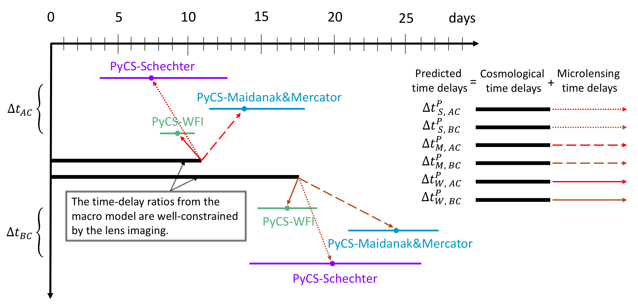
Figure 3 shows the posteriors of the constraints on the microlensing time delays and blinded with selected accretion disc configurations. The most constraining case (or the case with tightest prior on microlensing time delays), i.e., with size , , and PA , provides the best constraint on . In Figure 4, we show the fractional difference of . In panel (a), the top curve represents the case which ignores the microlensing time-delay effect and the two bottom curves represent the cases in which (1) we convolve the probability distribution of the loosest constraint of microlensing (size , , and PA ) with the probability distribution of the observed time-delays, (2) we simply add the uncertainty of the case with the loosest constraint on microlensing to the observed time-delay uncertainty in quadrature and shift the mean of the observed time-delay by the mean of the loosest case. In both cases, the constraint on are all looser than our method because both of them ignore the information from the cosmological time-delay ratios. The rest of the curves show the results in all different accretion disc configurations. Panel (a) provides two insights. First, the peaks gradually shift to larger when we increase the disc size. This makes sense as the larger the accretion disc is, the more positive the mean of the microlensing time-delay effect is (TK18). Second, the size of the accretion disc dominates the uncertainty of the inferred . Panel (b) shows the result which marginalizes all the different accretion disc configurations from panel (a).
4.1.2 The discrepant time-delay measurements in the different epochs
Even though the TDC has showed that the current PyCS curve shifting technique can remove the contamination from the “standard” microlensing magnification effect and accurately measure time delays, PyCS-WFI and PyCS-Maidanak are sigma discrepant. (see PyCS-Maidanak+Mercator, and PyCS-WFI in Figure 2) Thus, before TK18, this raised the question of how to combine the measurements
- •
First, we consider that we can measure the same cosmological delays on the three datasets, in which case we have three independent measurements of the delay that can be combined by multiplying their probability distribution functions. This is the PyCS-mult estimate in Figure 2.
- •
Second, we consider that microlensing is biasing our measurements on each dataset, in which case the combined estimate is obtained by marginalizing over the three measurements because we do not have information about the microlensing time-delay effect. This is the PyCS-sum in Figure 2.

Under the assumptions of TK18, the discrepancy in the time-delay measurements in the different epochs can be understood, as the microlensing time-delay effect can vary across ten to twenty years (Schechter & Wambsganss, 2002; Mosquera & Kochanek, 2011, e.g.,). Therefore, we should use neither PyCS-mult nor PyCS-sum. Instead, to deliver an unbiased measurement and make good use of information from the microlensing time-delay maps and the cosmological time-delay ratios, it is better to model each time-delay measurement with its own microlensing parameter sets. That is, Equation (3) should be expanded to
where
and the likelihood is
where the subscript “”, “”, and “” represents the time-delay measurements from PyCS-Schechter, PyCS-Maidanak+Mercator, and PyCS-WFI, respectively.
| parameters | ||||
|---|---|---|---|---|
| time delays [days] | ||||
| parameters | ||||
| time delays [days] | ||||
| parameters | ||||
| time delays [days] |
Equation (4.1.2) means that we have six measurements (two for each dataset) to constrain one and three sets of independent microlensing parameters (see Figure 5). We assume the three datasets share the same accretion disk configuration, , because the configuration of the accretion disc should stay invariant over the twenty years. We also follow Equation (4) to marginalize all the different source configurations and show the results in Table 2 and Figure 6. Table 2 shows that inferred probability distribution of the microlensing time delay parameters at the position of each lensed image in different datasets. Figure 6 shows the different values when we adopt PyCS-sum and “PyCS-Schechter&PyCS-Madanak+Mercator&PyCS-WFI”. Note that “PyCS-Schechter&PyCS-Madanak+Mercator&PyCS-WFI” indicates that we use three different microlensing parameter sets to model three different time delay measurements.


| parameters | ||||
|---|---|---|---|---|
| time delays [days] |
4.2 RXJ1131-1231
The RXJ 11311231 system is a quadruply-lensed quasar discovered by Sluse et al. (2003), who also measured the spectroscopic redshifts of lensing galaxy and the background source to be at and . Because of the long time delays ( days) of this lens system, Tewes et al. (2013b) can measure the time delay of image , with a fractional uncertainty of 1.5% () while the delays between the three close images , , and are compatible with being 0 days (i.e., days, days, days). Therefore, for RXJ 11311231, Equation (3) can be expressed as
We use the same , , and as TK18 to generate the microlensing time-delay maps given the combinations of different accretion disc sizes (, , and ), different to the line of slight ( and ), and different PA (, , and ) at the four lensed images. We show the constraint on in different accretion disc configurations in Figure 7 and the marginalized posteriors of the microlensing time delays in Table 3. As expected, the microlensing time-delay effect on the lens with longer time delays has less impact. In the case of RXJ 11311231, the impact by microlensing time-delay effect is negligible.
5 Conclusions
This paper quantifies the impact of microlensing time delays, produced under the assumption that AGN variability is the lamp-post type, on the time-delay distance. For that purpose we calculate the time-delay distance, , including the microlensing time-delay effect for two lens systems, PG 1115080 and RXJ 11311231, We find that this broadens the probability distribution by about 3% in the case of PG 1115080 and 0.1% in the case of RXJ 11311231.
Given the lamp-post model assumption, although we do not have any knowledge about how severely each light curve is affected by the microlensing time-delay effect, the cosmological time-delay ratios, which are well-constrained by the full surface brightness morphology of the lensed host galaxy emission, provide the constraining information on the possible combinations of the microlensing time delay at each lensed image position. Furthermore, the microlensing time-delay maps also provide constraints on the microlensing time-delay effect at each lensed image position. Thus, we have developed a new time-delay prediction model, which uses the information from cosmological time-delay ratios, as well as the information from microlensing time-delay maps, to remove the biases caused by this proposed effect under a Bayesian framework.
There are several key results:
- 1.
Under the assumption of TK18, different lens systems can yield different due to the fact that the measured time delays are not the cosmological time delays but the combination of cosmological time delays plus microlensing time delays. With this new time-delay prediction model, we can separately predict the cosmological time delays and microlensing time delays to measure a unbiased value of for each lens. Thus, this paper addresses concerns that TDSL have already hit the systematics floor in the time delay measurements due to this newly proposed microlensing time-delay effect, although it does increase the error budget.
- 2.
The time-delay measurements in different epochs should be modeled by different microlensing parameters as they are likely affected by different microlensing time-delay effects.
- 3.
Given a lens system, the constraint on mainly depends on the size of the accretion disc, whereas the inclination and the position angle of the disc have little influence. Thus, the smaller the disc is, the smaller the variances on the microlensing time delays are.
- 4.
The uncertainty on from PG 1115080, which has relatively short time delays, increases from % to % when we include the microlensing time-delay effects. Without our new technique, the uncertainty on from PG 1115080 can increase by up to 30%.
- 5.
The uncertainty on from RXJ 11311231, which has relatively long time delays, increases only from % to % when we include the microlensing time-delay effects. Thus, the impact of the microlensing time-delay effect on RXJ 11311231 is negligible.
Note that although we assume the lamp-post model on accretion disc, there is evidence (Morgan et al., 2010; Blackburne et al., 2011, e.g.,) showing that the size of the accretion disc is larger than the prediction from the standard thin disk theory. In addition, exist a variety of alternative accretion disc models (Beloborodov, 1999, e.g.,), including e.g. the inhomogeneous accretion disc (Dexter & Agol, 2011, e.g.,) for which variability is different from the lamp-post model.
As the amplitude of this effect highly depends on the accretion disk models, which are not well-understood, in our future determinations of from the H0LiCOW programme, we will present the measurements both with and without microlensing time-delay effects. The techniques for verifying the accretion disk models by using observational data are currently under development.
Finally, we want to stress that with the advantage of cosmological time-delay ratios, quads are better than doubles in term of constraining the microlensing time-delay effect in measuring the value of . The final measurements from PG 1115080 and RXJ 11311231 will be presented in Chen et al. 2018b in prep.
Acknowledgements
We thank Cristian E. Rusu and Stefan Hilbert for comments. G. C.-F. C. also thanks Chun-Hao To and Shih-Wei Chuo for technical discussions, and the UC Davis cosmology group for providing a friendly research environment. G. C.-F. C. acknowledges support from the Ministry of Education in Taiwan via Government Scholarship to Study Abroad (GSSA). G. C.-F. C. and C. D. F. acknowledge support from the National Science Foundation under grant AST-1715611. G. C.-F. C. and C. D. F. thank the Max Planck Institute for Astrophysics for kind hospitality during working visits. K.C.W. is supported by an EACOA Fellowship awarded by the East Asia Core Observatories Association, which consists of the Academia Sinica Institute of Astronomy and Astrophysics, the National Astronomical Observatory of Japan, the National Astronomical Observatories of the Chinese Academy of Sciences, and the Korea Astronomy and Space Science Institute. J. C., V. B., M. M., and F. C. are supported by the Swiss National Science Foundation. S. V. has received funding from the European Research Council (ERC) under the European Union’s Horizon 2020 research and innovation programme (grant agreement No 758853). L. V. E. K. are supported through an NWO-VICI grant (project number 639.043.308). S. H. S thanks the Max Planck Society for support through the Max Planck Research Group. A. J. S. and T. T. acknowledge support by NASA through STSCI grant HST-GO-15320, and by the Packard Foundation through a Packard Fellowship to T. T.
References
- Agnello (2017) Agnello A., 2017, preprint, (arXiv:1705.08900)
- Agnello et al. (2017) Agnello A., et al., 2017, preprint, (arXiv:1711.03971)
- Aubourg et al. (2015) Aubourg É., et al., 2015, Phys. Rev. D, 92, 123516
- Avestruz et al. (2017) Avestruz C., Li N., Lightman M., Collett T. E., Luo W., 2017, preprint, (arXiv:1704.02322)
- Beloborodov (1999) Beloborodov A. M., 1999, in Poutanen J., Svensson R., eds, Astronomical Society of the Pacific Conference Series Vol. 161, High Energy Processes in Accreting Black Holes. p. 295 (arXiv:astro-ph/9901108)
- Birrer et al. (2015) Birrer S., Amara A., Refregier A., 2015, ApJ, 813, 102
- Birrer et al. (2017) Birrer S., Welschen C., Amara A., Refregier A., 2017, J. Cosmology Astropart. Phys., 4, 049
- Blackburne et al. (2011) Blackburne J. A., Pooley D., Rappaport S., Schechter P. L., 2011, ApJ, 729, 34
- Bonvin et al. (2016) Bonvin V., Tewes M., Courbin F., Kuntzer T., Sluse D., Meylan G., 2016, A&A, 585, A88
- Bonvin et al. (2017) Bonvin V., et al., 2017, MNRAS, 465, 4914
- Chen et al. (2016) Chen G. C.-F., et al., 2016, MNRAS, 462, 3457
- Cheung et al. (2014) Cheung C. C., et al., 2014, ApJ, 782, L14
- Christian et al. (1987) Christian C. A., Crabtree D., Waddell P., 1987, ApJ, 312, 45
- Courbin et al. (2018) Courbin F., et al., 2018, A&A, 609, A71
- Dexter & Agol (2011) Dexter J., Agol E., 2011, ApJ, 727, L24
- Ding et al. (2018) Ding X., et al., 2018, preprint, (arXiv:1801.01506)
- Dobler et al. (2013) Dobler G., Fassnacht C., Treu T., Marshall P. J., Liao K., Hojjati A., Linder E., Rumbaugh N., 2013, preprint, (arXiv:1310.4830)
- Eulaers et al. (2013) Eulaers E., et al., 2013, A&A, 553, A121
- Falco et al. (1985) Falco E. E., Gorenstein M. V., Shapiro I. I., 1985, ApJ, 289, L1
- Fassnacht et al. (2002) Fassnacht C. D., Xanthopoulos E., Koopmans L. V. E., Rusin D., 2002, ApJ, 581, 823
- Fassnacht et al. (2011) Fassnacht C. D., Koopmans L. V. E., Wong K. C., 2011, MNRAS, 410, 2167
- Foreman-Mackey et al. (2013) Foreman-Mackey D., Hogg D. W., Lang D., Goodman J., 2013, PASP, 125, 306
- Freedman (2017) Freedman W. L., 2017, Nature Astronomy, 1, 0169
- Goodman & Weare (2010) Goodman J., Weare J., 2010, Communications in Applied Mathematics and Computational Science, Vol.˜5, No.˜1, p.˜65-80, 2010, 5, 65
- Henry & Heasley (1986) Henry J. P., Heasley J. N., 1986, Nature, 321, 139
- Hinshaw et al. (2013) Hinshaw G., et al., 2013, ApJS, 208, 19
- Hinton (2016) Hinton S. R., 2016, The Journal of Open Source Software, 1, 00045
- Jee et al. (2015) Jee I., Komatsu E., Suyu S. H., 2015, J. Cosmology Astropart. Phys., 11, 033
- Jee et al. (2016) Jee I., Komatsu E., Suyu S. H., Huterer D., 2016, J. Cosmology Astropart. Phys., 4, 031
- Joseph et al. (2014) Joseph R., et al., 2014, A&A, 566, A63
- Keeton & Moustakas (2009) Keeton C. R., Moustakas L. A., 2009, ApJ, 699, 1720
- Kochanek & Dalal (2004) Kochanek C. S., Dalal N., 2004, ApJ, 610, 69
- Komatsu et al. (2011) Komatsu E., et al., 2011, ApJS, 192, 18
- Koopmans (2005) Koopmans L. V. E., 2005, MNRAS, 363, 1136
- Koopmans et al. (2003) Koopmans L. V. E., Treu T., Fassnacht C. D., Blandford R. D., Surpi G., 2003, ApJ, 599, 70
- Lanusse et al. (2018) Lanusse F., Ma Q., Li N., Collett T. E., Li C.-L., Ravanbakhsh S., Mandelbaum R., Póczos B., 2018, MNRAS, 473, 3895
- Liao et al. (2015) Liao K., et al., 2015, ApJ, 800, 11
- Lin et al. (2017) Lin H., et al., 2017, ApJ, 838, L15
- Mao & Schneider (1998) Mao S., Schneider P., 1998, MNRAS, 295, 587
- Morgan et al. (2010) Morgan C. W., Kochanek C. S., Morgan N. D., Falco E. E., 2010, ApJ, 712, 1129
- Mosquera & Kochanek (2011) Mosquera A. M., Kochanek C. S., 2011, ApJ, 738, 96
- Nightingale & Dye (2015) Nightingale J. W., Dye S., 2015, MNRAS, 452, 2940
- Oguri (2010) Oguri M., 2010, PASJ, 62, 1017
- Oguri & Marshall (2010) Oguri M., Marshall P. J., 2010, MNRAS, 405, 2579
- Ostrovski et al. (2017) Ostrovski F., et al., 2017, MNRAS, 465, 4325
- Ostrovski et al. (2018) Ostrovski F., et al., 2018, MNRAS, 473, L116
- Peng et al. (2006) Peng C. Y., Impey C. D., Rix H.-W., Falco E. E., Keeton C. R., Kochanek C. S., Lehár J., McLeod B. A., 2006, New Astron. Rev., 50, 689
- Petrillo et al. (2017) Petrillo C. E., et al., 2017, MNRAS, 472, 1129
- Planck Collaboration et al. (2016) Planck Collaboration et al., 2016, A&A, 594, A13
- Plous (1993) Plous S., 1993, The Psychology of Judgment and Decision Making. McGraw-Hill Education, https://books.google.com/books?id=xvWOQgAACAAJ
- Rathna Kumar et al. (2013) Rathna Kumar S., et al., 2013, A&A, 557, A44
- Refsdal (1964) Refsdal S., 1964, MNRAS, 128, 307
- Riess et al. (1998) Riess A. G., et al., 1998, AJ, 116, 1009
- Riess et al. (2016) Riess A. G., et al., 2016, ApJ, 826, 56
- Rusu et al. (2017) Rusu C. E., et al., 2017, MNRAS, 467, 4220
- Schechter & Wambsganss (2002) Schechter P. L., Wambsganss J., 2002, ApJ, 580, 685
- Schechter et al. (1997) Schechter P. L., et al., 1997, ApJ, 475, L85
- Schechter et al. (2017) Schechter P. L., Morgan N. D., Chehade B., Metcalfe N., Shanks T., McDonald M., 2017, AJ, 153, 219
- Schneider & Sluse (2013) Schneider P., Sluse D., 2013, A&A, 559, A37
- Schneider & Sluse (2014) Schneider P., Sluse D., 2014, A&A, 564, A103
- Shajib et al. (2018) Shajib A. J., Treu T., Agnello A., 2018, MNRAS, 473, 210
- Shakura & Sunyaev (1973) Shakura N. I., Sunyaev R. A., 1973, A&A, 24, 337
- Sluse et al. (2003) Sluse D., et al., 2003, A&A, 406, L43
- Suyu (2012) Suyu S. H., 2012, ArXiv e-prints (1202.0287),
- Suyu et al. (2010) Suyu S. H., Marshall P. J., Auger M. W., Hilbert S., Blandford R. D., Koopmans L. V. E., Fassnacht C. D., Treu T., 2010, ApJ, 711, 201
- Suyu et al. (2018) Suyu S. H., Chang T.-C., Courbin F., Okumura T., 2018, preprint, (arXiv:1801.07262)
- Tewes et al. (2013a) Tewes M., Courbin F., Meylan G., 2013a, A&A, 553, A120
- Tewes et al. (2013b) Tewes M., et al., 2013b, A&A, 556, A22
- Tie & Kochanek (2018) Tie S. S., Kochanek C. S., 2018, MNRAS, 473, 80
- Tihhonova et al. (2017) Tihhonova O., et al., 2017, preprint, (arXiv:1711.08804)
- Tonry (1998) Tonry J. L., 1998, AJ, 115, 1
- Treu & Koopmans (2002) Treu T., Koopmans L. V. E., 2002, MNRAS, 337, L6
- Treu & Marshall (2016) Treu T., Marshall P. J., 2016, A&ARv, 24, 11
- Tsvetkova et al. (2010) Tsvetkova V. S., et al., 2010, MNRAS, 406, 2764
- Vegetti & Koopmans (2009) Vegetti S., Koopmans L. V. E., 2009, MNRAS, 392, 945
- Wambsganss (2006) Wambsganss J., 2006, ArXiv Astrophysics e-prints,
- Warren & Dye (2003) Warren S. J., Dye S., 2003, ApJ, 590, 673
- Weinberg et al. (2013) Weinberg D. H., Mortonson M. J., Eisenstein D. J., Hirata C., Riess A. G., Rozo E., 2013, Phys. Rep., 530, 87
- Williams et al. (2018) Williams P. R., et al., 2018, MNRAS,
- Wong et al. (2017) Wong K. C., et al., 2017, MNRAS, 465, 4895
- Xu et al. (2015) Xu D., Sluse D., Schneider P., Springel V., Vogelsberger M., Nelson D., Hernquist L., 2015, ArXiv:1507.07937,
- de Grijs et al. (2017) de Grijs R., Courbin F., Martínez-Vázquez C. E., Monelli M., Oguri M., Suyu S. H., 2017, Space Sci. Rev., 212, 1743