Dynamical Quantum Phase Transitions: A Geometric Picture
Abstract
The Loschmidt echo (LE) is a purely quantum-mechanical quantity whose determination for large quantum many-body systems requires an exceptionally precise knowledge of all eigenstates and eigenenergies. One might therefore be tempted to dismiss the applicability of any approximations to the underlying time evolution as hopeless. However, using the fully connected transverse-field Ising model (FC-TFIM) as an example, we show that this indeed is not the case, and that a simple semiclassical approximation to systems well described by mean-field theory (MFT) is in fact in good quantitative agreement with the exact quantum-mechanical calculation. Beyond the potential to capture the entire dynamical phase diagram of these models, the method presented here also allows for an intuitive geometric interpretation of the fidelity return rate at any temperature, thereby connecting the order parameter dynamics and the Loschmidt echo in a common framework. Videos of the post-quench dynamics provided in the supplemental material visualize this new point of view.
Equilibrium phase transitions are remarkable phenomena that have been under thorough experimental and theoretical investigation for decades. Over time, a number of advanced techniques such as scaling theory [1, 2, 3] and the renormalization group method [4, 5, 6, 7, 8, 9] have been developed for the determination of the universal properties close to a critical point. One might ask whether an in-depth study of dynamical critical phenomena far from equilibrium is possible along the lines established in the equilibrium framework. With the advent of modern ultracold atom [10, 11, 12, 13] and ion-trap [14, 15, 16] experiments, this originally purely academic question has become accessible in laboratories as well.
Dynamical quantum phase transitions (DPTs) occur in the dynamics of a quantum system after quenching a set of control parameters of its Hamiltonian: . Recently, the study of DPTs has focused on two largely independent concepts [17]. The first one, DPT-I [18, 19, 20, 21, 22, 23, 24, 25, 26, 27, 28, 29], resembles equilibrium Landau theory: A system undergoes a dynamical phase transition if the long-time limit of the order parameter is finite for one set , whereas it vanishes for different final parameters . Furthermore, DPT-I also entails criticality in the transient dynamics of the order parameter and two-point correlators before reaching the steady state, giving rise to effects such as dynamic scaling and aging, which have been investigated theoretically [30, 31, 32] and also observed experimentally [33].
The second concept, DPT-II, generalizes the non-analytic behavior of the free energy at a phase transition in the thermodynamic limit (TL) to the out-of-equilibrium case. To this end, the LE has been introduced as a dynamical analog of a free energy per particle [34]. DPT-II has been extensively studied both theoretically [34, 35, 36, 37, 38, 39, 40, 41, 42, 43] and in experiments [44, 45]. As we aim to calculate dynamical phase transitions at finite preparation temperatures, we define the distance covered in Hilbert space between the pre-quench density matrix and the time-evolved in the limit of infinite system size as the fidelity return rate [46, 47, 48, 49]
| (1) |
For , the return rate reduces to the original definition [34]. Within our semiclassical theory we will find a simple and intuitive expression for the distance measure (1).
DPT-II is characterized by cusps occurring in at critical times after a quench. There are two scenarios for these cusps. The first is when the argument of the logarithm is zero, which is encountered only at [46] in two-band models of free fermions [50, 51, 40], when for critical quasi-momenta the population becomes inverted [39]. Upon integration over -space the resulting logarithmic divergence will be turned into a cusp. Alternatively, the argument of the logarithm may itself become nonanalytic [52, 53], which occurs for example in nonintegrable quantum Ising chains with ferromagnetic power-law interactions [54, 55, 56, 57]. At , numerical investigations have shown a relationship between the DPT-I and DPT-II in the presence of sufficiently long-range interactions [52, 58, 53, 59]. At finite temperatures the DPT-I and DPT-II phase diagram based on coincide for the FC-TFIM [60].
Of course, like for equilibrium phase transitions, a perfectly sharp cusp of any LE will only be observable in the TL. An accurate determination of the LE in this limit, however, requires computation of overlaps between different eigenstates to a precision that grows exponentially with system size. On the one hand, this sensitive dependence on complicates numerical treatment of large systems necessary for a reliable finite-size scaling, and, on the other hand, it may seem to completely rule out any kind of perturbative expansion with algebraic corrections. Here we show otherwise.
As we will discuss in detail in the case of the FC-TFIM, for models where MFT can be applied, one can create a controlled, semiclassical extension to the solution of the mean-field equations, which accurately reproduces the full return function and in particular determines the DPT-II phases correctly. In fact, a closely related analysis has already successfully explained the collapse and revival of the time-of-flight interference patterns following a quench to the deep lattice limit of the Bose-Hubbard model [13]. The Hamiltonian of the FC-TFIM, also known as the LMG model in nuclear physics [61, 62, 63, 64, 65, 66], reads
| (2) |
where are the Pauli matrices on site . The normalization ensures extensive scaling of the energy. Furthermore, we set the ferromagnetic coupling to unity. In order to study the DPT-II induced by quenches in the transverse-field strength , we utilize the infinite-range interaction to rewrite the Hamiltonian in terms of the total spin :
| (3) |
which is exact up to an irrelevant constant. Due to , the total spin length is conserved, even after the quench .
For this quench protocol, the DPT-I phase diagram for is completely determined by MFT [21], which is equivalent to the leading order of a -expansion. It is based on the Bloch sphere representation of the spin in terms of the continuous classical vector that contributes the highest weight to the free energy arising from the pre-quench Hamilton function
| (4) |
The short-time evolution is then governed by the classical equations of motion (EOM) derived from the post-quench Hamiltonian ; see (6) below. The MFT thus forms the starting point for the semiclassical treatment of the LE and the DPT-II phase diagram, the construction of which we will now detail. For simplicity, we restrict ourselves to in the rest of the manuscript. Initially, we focus on the zero-temperature case and deal with thermal states later.
At , one first finds the vector minimizing , which we choose, due to the spontaneously broken symmetry, to be fully polarized along the positive -axis. In other words, has angular variables , arbitrary, and the maximal possible length . For later convenience we also introduce , so here .
Next we have to quantize our theory in order to define the notion of overlaps between different states, which inherently arises from quantum mechanics. To do so, we assign to the spin WKB wave function [3, 68, 4] of a quantum mechanical degree of freedom in the ground state of the energy landscape :
| (5) | ||||
where is an inconsequential normalization; see SM. To enforce symmetry breaking, we restrict to the northern hemisphere. By construction correctly determines the fluctuations and with next-to-leading order corrections in .


Having set up the semiclassical state at time , we now incorporate the time evolution with by first determining the classical trajectories of the angular variables , which result from the classical EOM
| (6) |
with initial conditions . These derive from the Heisenberg equations for the total spin operators by neglecting all commutators that are suppressed by at least [60]. In close analogy to the time evolution in a truncated Wigner approximation [70], the initial amplitude is then transported along the classical trajectory, which implies that depends on both initial angles and . Due to the absence of any dephasing within this description the magnetization, however, will never relax. Higher-order corrections can be treated by more faithfully representing the Schrödinger equation on the Bloch sphere, which will then include derivatives acting on the wave function (5) [21]. Here we take no effects beyond (6) into account, which will turn out to determine the critical times accurately. In this limit the Loschmidt return function at , defined in (1), reads
| (7) | ||||
where the integral sums over the surface of the Bloch sphere with measure . The simple expression in the second line results from the limit , where, due to the extensive scaling of the exponent of the wave function (5), at every moment in time the integral is determined by the Loschmidt vector corresponding to the saddle-point trajectory that minimizes the exponent. Note that, as depicted in the SM, the initial coordinates are themselves time dependent. Furthermore, this result allows for a simple geometric interpretation: The classical trajectory with smallest arithmetic mean of initial and time-evolved WKB distances from the classical initial state dominates the LE.
To compute according to (7), we cover the Bloch sphere with a Fibonacci lattice, assigning to each point the corresponding WKB amplitude of (5). This lattice is then evolved in time, by numerically solving (6) and finally extracting the site that yields the largest contribution to .
Figures 1 and 2 illustrate our results for the spin dynamics in case of quenches to and shortly after the first critical time. The corresponding return rates can be found in Figs. 4 a) and b). Movies of the spin dynamics are attached as video supplemental [71, 72, 73]. The first quench is known to lie within the anomalous phase (no cusp in the first period(s) of ) whereas the latter gives rise to a regular signal (all periods show non-analyticities) [52].
In the anomalous quench to [71], the classical state moves only in the upper hemisphere yielding a positive at all times. Consequently, its trajectory returns so quickly to the initial state that the wave packet remains sufficiently concentrated around the classical state to prevent any discontinuous movement of the Loschmidt vector (obtained from (7)) during the first period. The first jump of , and therefore cusp in , appears only in the second period in agreement with the results obtained by ED calculations (see Fig. 4). At very late times the initial wave packet has spread so far over the Bloch sphere that the Loschmidt vector always points near the north pole, resulting in a very small .
For the regular quench to on the other hand [72], the classical vector crosses the equator of the Bloch sphere where the increased fluctuations in result in a fast squeezing of the wave packet. This gives rise to a jump of the dominant orientation already during the first period of the motion, and thus to a regular LE.
The semiclassical evolution, therefore, allows for a very intuitive understanding of the relation between the order parameter dynamics and the return rate.
Let us now consider finite temperatures where the initial classical state for minimizes the mean-field free energy
| (8) |
where
| (9) |
denotes the degeneracy of the spin subspace of length . These two equations specify the mean-field pre-quench state in terms of with and arbitrary [60]. The exact initial density matrix in the eigenbasis of in our semiclassical description becomes
| (10) |
where the generalization of the WKB wave function in (5) to an arbitrary eigenenergy reads
| (11) |
Here, is an inconsequential static normalization and , , and are functions of and , where the latter seperates the classically allowed () from the forbidden region (see SM for the derivation). In the TL the off-diagonal terms in (10) are suppressed by factors exponentially large in the system size and thus we can set .
Using this diagonal form of and the fact that the truncated time evolution acts only on the coordinates , we can write for the fidelity LE ; cf. (1). In the TL the remaining integrals in this expression once again reduce to their saddle-point values, equivalent to the minimization problem over all starting points in
| (12) |
and all classical angles in the combined thermal and WKB distance measure
| (13) |
The geometric interpretation of (12) remains the same as in (7), but now first finds the saddle point of the density matrix, i.e. the largest product of the wave function and the corresponding Boltzmann factor .
We illustrate the dynamics on the Bloch sphere for a quench to [73] at in Fig. 3 and the corresponding LE in Fig. 4. The initial state shows a finite magnetization but the radius of the Bloch sphere has decreased to . Due to the thermal fluctuations the quench is now regular and, in contrast to the case, shows the same features as Fig. 2. This can be explained by the decreased spin length which effectively renders the transverse field in the Hamiltonian more relevant compared to the -term. As a result, the ground state of the final Hamiltonian is paramagnetic and the quench crosses the ferro- to paramagnetic transition in the DPT-I picture as well.
Finally, note that for high temperatures close to the equilibrium critical temperature the initial distribution on the Bloch sphere becomes fully determined by thermal fluctuations. Hence, in (12) can then by replaced by the completely thermal distance measure
| (14) |
As evidenced in Fig. 4c) this simplification already produces decent results for the quench considered in Fig. 3, where we are thus calculating an essentially classical return rate.
Conclusion.–We have shown, using the example of the FC-TFIM, that for systems where the short-time dynamics is well described by MFT, the LE at zero temperature can be described to a high degree of accuracy by a semiclassical approximation. At sufficiently high temperatures, even a purely classical thermal cloud yields a qualitative reproduction of the fidelity LE that is otherwise difficult to obtain for large systems. This is remarkable since the implied approximations completely discard all dephasing, thereby prohibiting the system to relax at late times. The method also paves the way for the calculation of LEs or entanglement witnesses like Fisher information [74, 75, 76, 77] within the more general framework of the truncated Wigner approximation.
Acknowledgments.–We thank Francesco Piazza and Wilhelm Zwerger for fruitful comments on the manuscript. This project has been supported by NIM (Nanosystems Initiative Munich).
References
- [1] S. Ma, Statistical Mechanics (World Scientific, 1985), ISBN 9789971966065, URL https://books.google.de/books?id=YW-0AQAACAAJ.
- [2] J. Cardy, Scaling and Renormalization in Statistical Physics, Cambridge Lecture Notes in Physics (Cambridge University Press, 1996), ISBN 9780521499590, URL https://books.google.de/books?id=Wt804S9FjyAC.
- [3] S. Sachdev, Quantum Phase Transitions (Cambridge University Press, 2001), ISBN 9780521004541, URL https://books.google.de/books?id=Ih_E05N5TZQC.
- [4] K. G. Wilson, Phys. Rev. B 4, 3174 (1971a), URL https://link.aps.org/doi/10.1103/PhysRevB.4.3174.
- [5] K. G. Wilson, Phys. Rev. B 4, 3184 (1971b), URL https://link.aps.org/doi/10.1103/PhysRevB.4.3184.
- [6] K. G. Wilson and M. E. Fisher, Phys. Rev. Lett. 28, 240 (1972), URL https://link.aps.org/doi/10.1103/PhysRevLett.28.240.
- [7] K. G. Wilson and J. Kogut, Physics Reports 12, 75 (1974), ISSN 0370-1573, URL http://www.sciencedirect.com/science/article/pii/0370157374900234.
- [8] M. E. Fisher, Rev. Mod. Phys. 46, 597 (1974), URL https://link.aps.org/doi/10.1103/RevModPhys.46.597.
- [9] K. G. Wilson, Rev. Mod. Phys. 47, 773 (1975), URL https://link.aps.org/doi/10.1103/RevModPhys.47.773.
- [10] K. Levin, A. Fetter, and D. Stamper-Kurn, Ultracold Bosonic and Fermionic Gases, Contemporary Concepts of Condensed Matter Science (Elsevier Science, 2012), ISBN 9780444538628, URL https://books.google.de/books?id=rLlplpMuX6oC.
- [11] V. I. Yukalov, Laser Physics Letters 8, 485 (2011), URL http://stacks.iop.org/1612-202X/8/i=7/a=001.
- [12] I. Bloch, J. Dalibard, and W. Zwerger, Rev. Mod. Phys. 80, 885 (2008), URL https://link.aps.org/doi/10.1103/RevModPhys.80.885.
- [13] M. Greiner, O. Mandel, T. W. Hänsch, and I. Bloch, Nature 419, 51-54 (2002), URL https://www.nature.com/articles/nature00968.
- [14] D. Porras and J. I. Cirac, Phys. Rev. Lett. 92, 207901 (2004), URL https://link.aps.org/doi/10.1103/PhysRevLett.92.207901.
- [15] K. Kim, M.-S. Chang, R. Islam, S. Korenblit, L.-M. Duan, and C. Monroe, Phys. Rev. Lett. 103, 120502 (2009), URL https://link.aps.org/doi/10.1103/PhysRevLett.103.120502.
- [16] P. Jurcevic, B. P. Lanyon, P. Hauke, C. Hempel, P. Zoller, R. Blatt, and C. F. Roos, Nature 511, 202-205 (2014), URL http://www.nature.com/articles/nature13461.
- [17] A. A. Zvyagin, Low Temperature Physics 42, 971 (2016), URL https://aip.scitation.org/doi/10.1063/1.4969869.
- [18] M. Moeckel and S. Kehrein, Phys. Rev. Lett. 100, 175702 (2008), URL https://link.aps.org/doi/10.1103/PhysRevLett.100.175702.
- [19] M. Moeckel and S. Kehrein, New Journal of Physics 12, 055016 (2010), URL http://stacks.iop.org/1367-2630/12/i=5/a=055016.
- [20] B. Sciolla and G. Biroli, Phys. Rev. Lett. 105, 220401 (2010), URL https://link.aps.org/doi/10.1103/PhysRevLett.105.220401.
- [21] B. Sciolla and G. Biroli, Journal of Statistical Mechanics: Theory and Experiment 2011, P11003 (2011), URL http://stacks.iop.org/1742-5468/2011/i=11/a=P11003.
- [22] A. Gambassi and P. Calabrese, EPL (Europhysics Letters) 95, 66007 (2011), URL http://stacks.iop.org/0295-5075/95/i=6/a=66007.
- [23] B. Sciolla and G. Biroli, Phys. Rev. B 88, 201110 (2013), URL https://link.aps.org/doi/10.1103/PhysRevB.88.201110.
- [24] A. Maraga, A. Chiocchetta, A. Mitra, and A. Gambassi, Phys. Rev. E 92, 042151 (2015), URL https://link.aps.org/doi/10.1103/PhysRevE.92.042151.
- [25] A. Chandran, A. Nanduri, S. S. Gubser, and S. L. Sondhi, Phys. Rev. B 88, 024306 (2013), URL https://link.aps.org/doi/10.1103/PhysRevB.88.024306.
- [26] P. Smacchia, M. Knap, E. Demler, and A. Silva, Phys. Rev. B 91, 205136 (2015), URL https://link.aps.org/doi/10.1103/PhysRevB.91.205136.
- [27] J. C. Halimeh, V. Zauner-Stauber, I. P. McCulloch, I. de Vega, U. Schollwöck, and M. Kastner, Phys. Rev. B 95, 024302 (2017), URL https://link.aps.org/doi/10.1103/PhysRevB.95.024302.
- [28] T. Mori, T. N. Ikeda, E. Kaminishi, and M. Ueda, ArXiv e-prints (2017), eprint 1712.08790, URL https://arxiv.org/abs/1712.08790.
- [29] J. Zhang, G. Pagano, P. W. Hess, A. Kyprianidis, P. Becker, H. Kaplan, A. V. Gorshkov, Z.-X. Gong, and C. Monroe, Nature 551, 601 (2017), URL https://www.nature.com/articles/nature24654.
- [30] A. Chiocchetta, M. Tavora, A. Gambassi, and A. Mitra, Phys. Rev. B 91, 220302 (2015), URL https://link.aps.org/doi/10.1103/PhysRevB.91.220302.
- [31] M. Marcuzzi, J. Marino, A. Gambassi, and A. Silva, Phys. Rev. B 94, 214304 (2016), URL https://link.aps.org/doi/10.1103/PhysRevB.94.214304.
- [32] A. Chiocchetta, A. Gambassi, S. Diehl, and J. Marino, Phys. Rev. Lett. 118, 135701 (2017), URL https://link.aps.org/doi/10.1103/PhysRevLett.118.135701.
- [33] E. Nicklas, M. Karl, M. Höfer, A. Johnson, W. Muessel, H. Strobel, J. Tomkovič, T. Gasenzer, and M. K. Oberthaler, Phys. Rev. Lett. 115, 245301 (2015), URL https://link.aps.org/doi/10.1103/PhysRevLett.115.245301.
- [34] M. Heyl, A. Polkovnikov, and S. Kehrein, Phys. Rev. Lett. 110, 135704 (2013), URL https://link.aps.org/doi/10.1103/PhysRevLett.110.135704.
- [35] M. Heyl, Phys. Rev. Lett. 113, 205701 (2014), URL https://link.aps.org/doi/10.1103/PhysRevLett.113.205701.
- [36] F. Andraschko and J. Sirker, Phys. Rev. B 89, 125120 (2014), URL https://link.aps.org/doi/10.1103/PhysRevB.89.125120.
- [37] S. Vajna and B. Dóra, Phys. Rev. B 89, 161105 (2014), URL https://link.aps.org/doi/10.1103/PhysRevB.89.161105.
- [38] M. Heyl, Phys. Rev. Lett. 115, 140602 (2015), URL https://link.aps.org/doi/10.1103/PhysRevLett.115.140602.
- [39] S. Vajna and B. Dóra, Phys. Rev. B 91, 155127 (2015), URL https://link.aps.org/doi/10.1103/PhysRevB.91.155127.
- [40] J. C. Budich and M. Heyl, Phys. Rev. B 93, 085416 (2016), URL https://link.aps.org/doi/10.1103/PhysRevB.93.085416.
- [41] U. Bhattacharya, S. Bandyopadhyay, and A. Dutta, Phys. Rev. B 96, 180303 (2017), URL https://link.aps.org/doi/10.1103/PhysRevB.96.180303.
- [42] M. Heyl and J. C. Budich, Phys. Rev. B 96, 180304 (2017), URL https://link.aps.org/doi/10.1103/PhysRevB.96.180304.
- [43] M. Heyl, Reports on Progress in Physics 81, 054001 (2018), URL http://stacks.iop.org/0034-4885/81/i=5/a=054001.
- [44] N. Fläschner, D. Vogel, M. Tarnowski, B. S. Rem, D.-S. Lühmann, M. Heyl, J. C. Budich, L. Mathey, K. Sengstock, and C. Weitenberg, Nature Physics 14, 265 (2018), ISSN 1745-2481, URL https://doi.org/10.1038/s41567-017-0013-8.
- [45] P. Jurcevic, H. Shen, P. Hauke, C. Maier, T. Brydges, C. Hempel, B. P. Lanyon, M. Heyl, R. Blatt, and C. F. Roos, Phys. Rev. Lett. 119, 080501 (2017), URL https://link.aps.org/doi/10.1103/PhysRevLett.119.080501.
- [46] N. Sedlmayr, M. Fleischhauer, and J. Sirker, Phys. Rev. B 97, 045147 (2018), URL https://link.aps.org/doi/10.1103/PhysRevB.97.045147.
- [47] B. Mera, C. Vlachou, N. Paunković, V. R. Vieira, and O. Viyuela, Phys. Rev. B 97, 094110 (2018), URL https://link.aps.org/doi/10.1103/PhysRevB.97.094110.
- [48] P. Zanardi, H. T. Quan, X. Wang, and C. P. Sun, Phys. Rev. A 75, 032109 (2007), URL https://link.aps.org/doi/10.1103/PhysRevA.75.032109.
- [49] L. Campos Venuti, N. T. Jacobson, S. Santra, and P. Zanardi, Phys. Rev. Lett. 107, 010403 (2011), URL https://link.aps.org/doi/10.1103/PhysRevLett.107.010403.
- [50] Z. Huang and A. V. Balatsky, Phys. Rev. Lett. 117, 086802 (2016), URL https://link.aps.org/doi/10.1103/PhysRevLett.117.086802.
- [51] A. Dutta and A. Dutta, Phys. Rev. B 96, 125113 (2017), URL https://link.aps.org/doi/10.1103/PhysRevB.96.125113.
- [52] J. C. Halimeh and V. Zauner-Stauber, Phys. Rev. B 96, 134427 (2017), URL https://link.aps.org/doi/10.1103/PhysRevB.96.134427.
- [53] V. Zauner-Stauber and J. C. Halimeh, Phys. Rev. E 96, 062118 (2017), URL https://link.aps.org/doi/10.1103/PhysRevE.96.062118.
- [54] A. Dutta and J. K. Bhattacharjee, Phys. Rev. B 64, 184106 (2001), URL https://link.aps.org/doi/10.1103/PhysRevB.64.184106.
- [55] M. Knap, A. Kantian, T. Giamarchi, I. Bloch, M. D. Lukin, and E. Demler, Phys. Rev. Lett. 111, 147205 (2013), URL https://link.aps.org/doi/10.1103/PhysRevLett.111.147205.
- [56] D. Jaschke, K. Maeda, J. D. Whalen, M. L. Wall, and L. D. Carr, New Journal of Physics 19, 033032 (2017), URL http://stacks.iop.org/1367-2630/19/i=3/a=033032.
- [57] L. Vanderstraeten, M. Van Damme, H. P. Büchler, and F. Verstraete, ArXiv e-prints (2018), eprint 1801.00769, URL https://arxiv.org/abs/1801.00769.
- [58] I. Homrighausen, N. O. Abeling, V. Zauner-Stauber, and J. C. Halimeh, Phys. Rev. B 96, 104436 (2017), URL https://link.aps.org/doi/10.1103/PhysRevB.96.104436.
- [59] B. Žunkovič, M. Heyl, M. Knap, and A. Silva, Phys. Rev. Lett. 120, 130601 (2018), URL https://link.aps.org/doi/10.1103/PhysRevLett.120.130601.
- [60] J. Lang, B. Frank, and J. C. Halimeh, Phys. Rev. B 97, 174401 (2018), URL https://link.aps.org/doi/10.1103/PhysRevB.97.174401.
- [61] H. Lipkin, N. Meshkov, and A. Glick, Nuclear Physics 62, 188 (1965), ISSN 0029-5582, URL http://www.sciencedirect.com/science/article/pii/002955826590862X.
- [62] N. Meshkov, A. Glick, and H. Lipkin, Nuclear Physics 62, 199 (1965), ISSN 0029-5582, URL http://www.sciencedirect.com/science/article/pii/0029558265908631.
- [63] A. Glick, H. Lipkin, and N. Meshkov, Nuclear Physics 62, 211 (1965), ISSN 0029-5582, URL http://www.sciencedirect.com/science/article/pii/0029558265908643.
- [64] R. Botet, R. Jullien, and P. Pfeuty, Phys. Rev. Lett. 49, 478 (1982), URL https://link.aps.org/doi/10.1103/PhysRevLett.49.478.
- [65] R. Botet and R. Jullien, Phys. Rev. B 28, 3955 (1983), URL https://link.aps.org/doi/10.1103/PhysRevB.28.3955.
- [66] P. Ribeiro, J. Vidal, and R. Mosseri, Phys. Rev. E 78, 021106 (2008), URL https://link.aps.org/doi/10.1103/PhysRevE.78.021106.
- [67] J. L. van Hemmen and A. Sütő, Physica B+C 141, 37 (1986), ISSN 0378-4363, URL http://www.sciencedirect.com/science/article/pii/0378436386903475.
- [68] P. A. Braun, Rev. Mod. Phys. 65, 115 (1993), URL https://link.aps.org/doi/10.1103/RevModPhys.65.115.
- [69] J. L. van Hemmen and A. Sütő, Physica A: Statistical Mechanics and its Applications 321, 493 (2003), ISSN 0378-4371, URL http://www.sciencedirect.com/science/article/pii/S0378437102015893.
- [70] A. Polkovnikov, Annals of Physics 325, 1790 (2010), ISSN 0003-4916, URL http://www.sciencedirect.com/science/article/pii/S0003491610000382.
- [71] https://youtu.be/gE72RBlWZ-c.
- [72] https://youtu.be/fUueTOyI2S4.
- [73] https://youtu.be/e8JhRAY-qbg.
- [74] M. G. A. Paris, International Journal of Quantum Information 07, 125 (2009), URL https://www.worldscientific.com/doi/abs/10.1142/S0219749909004839.
- [75] U. Marzolino and T. c. v. Prosen, Phys. Rev. A 90, 062130 (2014), URL https://link.aps.org/doi/10.1103/PhysRevA.90.062130.
- [76] U. Marzolino and T. c. v. Prosen, Phys. Rev. B 96, 104402 (2017), URL https://link.aps.org/doi/10.1103/PhysRevB.96.104402.
- [77] D. Braun, G. Adesso, F. Benatti, R. Floreanini, U. Marzolino, M. W. Mitchell, and P. S., ArXiv e-prints (2017), eprint 1701.05152, URL https://arxiv.org/abs/1701.05152.
— Supplemental Material —
Dynamical Quantum Phase Transitions: A Geometric Picture
Johannes Lang, Bernhard Frank, and Jad C. Halimeh
I Construction of the WKB wave function
In this supplement, we present the construction of the WKB wave function [1, 2] adapted to large spins [3, 4] for our initial Hamiltonian that reads [5]
| (S1) |
At first glance, it may seem as a complete technical overkill to create a semiclassical approximation to the eigenstates of the exactly solvable . However, the spin WKB wave functions can both be easily mapped onto the Bloch sphere, and, when expressed in terms of the eigenstates of with , they reproduce the correct fluctuations expressed by the expectation values of the quadratic spin operators [6]. Choosing the quantization axis along the -direction transforms the Hamiltonian to , where denotes the spin raising (lowering) operator. The stationary Schrödinger equation for with eigenenergy becomes the finite-difference equation
| (S2) |
with boundary condition . Here, we have omitted corrections of order from the exact prefactors of the raising and lowering operators and instead approximated them by . For the wave function, we use the WKB ansatz
| (S3) |
where denotes the normalization. Inserting this ansatz into the Schrödinger equation (S2) and making use of the fact that in the semiclassical limit the argument of can be treated as a continuous variable, one obtains to lowest order in
| (S4) |
where the prime indicates the derivative with respect to . In order to control the spin fluctuations described by the wave function with sufficient accuracy, however, it is necessary to extend the given solution by higher derivatives and thus the next-to-leading order in , which we parametrize as
| (S5) |
The correction term has to satisfy the condition
| (S6) |
which follows from the inclusion of the second derivative of in the continuum limit of the difference equation (S2) when acting on the ansatz (S3) with modified exponent (S5). This expression is only a good approximation if , which according to (S4) breaks down at the boundary of the classically allowed region. One thus has to expand around the maximally forbidden spin projections on the northern hemisphere (our choice for the broken symmetry), where successively higher derivatives are suppressed by increasing powers of . For energies close to the ground state energy one obtains
| (S7) |
showing that is indeed a correction to the leading terms. With this addition,
| (S8) |
is now consistent with the Schrödinger equation expanded up to the second derivative at all possible values of .
The reason behind the implementation of this non-standard WKB ansatz including is that it changes the boundary between the classically allowed and forbidden spin orientations from to the far more accurate
| (S9) |
which vanishes for the ground state as all higher-energy spin projections can only be reached via quantum tunneling through the classically forbidden region. To obtain the final expression for used for the determination of the Loschmidt return rate, one has to integrate (S3) with fixed lower boundary . Expanding around and using the asymptotics in the vicinity of , results in
| (S10) |

Here, we have introduced the abbreviations and , and the normalization is actually irrelevant for the determination of the Loschmidt return function. Quite importantly, shows the proper scaling of the spin expectations values, i.e. for the ground state and with subleading corrections. For the geometric interpretation outlined in the main text, placing these wave functions on the Bloch sphere is simply done by substituting , where is the polar angle on the Bloch sphere. Using the definitions for and , can be further simplified into the expression (11) given in the main text. In particular, at , one has and yielding (5) in the main text. A resolution of the azimuthal angle is not necessary as the rotational symmetry of the Hamiltonian will be recovered in any eigenfunction.
II Non-analytic dynamics of the Loschmidt vector
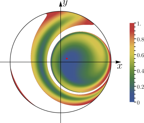
In the main text we have argued that the Loschmidt return rate is dominated by a single trajectory on the Bloch sphere, namely the Loschmidt vector , which can be obtained by minimizing a semi-classical distance measure. Here, we give further details on this geometric interpretation using the example of the anomalous quench from to at zero temperature. We show the angular distribution of the corresponding distance measure in Fig. S1, just before and after the critical time , when the first cusp in occurs (cf. Fig. 4 in the main text). At this time one of the local minima (blue regions) becomes the new global one, which causes a jump of (red dot). This discontinuous movement is directly related to the non-analyticity of .
In Fig. S2 we illustrate the initial orientation which is found when one evolves backwards in time. In agreement with the jump of the Loschmidt vector, we observe a sudden change of at the critical time.
References
- [1] K. Gottfried and T. Yan, Quantum Mechanics: Fundamentals, Graduate Texts in Contemporary Physics (Springer New York, 2003), ISBN 9780387955766, URL https://books.google.de/books?id=8gFX-9YcvIYC.
- [2] A. Messiah, Quantum Mechanics, Dover books on physics (Dover Publications, 1961), ISBN 9780486409245, URL https://books.google.de/books?id=mwssSDXzkNcC.
- [3] J. L. van Hemmen and A. Sütő, Physica B+C 141, 37 (1986), ISSN 0378-4363, URL http://www.sciencedirect.com/science/article/pii/0378436386903475.
- [4] J. L. van Hemmen and A. Sütő, Physica A: Statistical Mechanics and its Applications 321, 493 (2003), ISSN 0378-4371, URL http://www.sciencedirect.com/science/article/pii/S0378437102015893.
- [5] Cf. (3) in the main text with .
- [6] The obvious, direct representation in the eigenbasis of always yields too small fluctuations due to the vanishing width of the WKB wave functions as is diagonal in that particular basis.