Learning Software Constraints via Installation Attempts Thanks: The research leading to these results has received funding from the European Union under the H2020 and 5G-PPP Phase2 programs, under Grant Agreement No. 761 557 (project NGPaaS).
Abstract
Modern software systems are expected to be secure and contain all the latest features, even when new versions of software are released multiple times an hour. Each system may include many interacting packages. The problem of installing multiple dependent packages has been extensively studied in the past, yielding some promising solutions that work well in practice. However, these assume that the developers declare all the dependencies and conflicts between the packages. Oftentimes, the entire repository structure may not be known upfront, for example when packages are developed by different vendors. In this paper we present algorithms for learning dependencies, conflicts and defective packages from installation attempts. Our algorithms use combinatorial data structures to generate queries that test installations and discover the entire dependency structure. A query that the algorithms make corresponds to trying to install a subset of packages and getting a Boolean feedback on whether all constraints were satisfied in this subset. Our goal is to minimize the query complexity of the algorithms. We prove lower and upper bounds on the number of queries that these algorithms require to make for different settings of the problem.
1 Introduction
Modern software systems are very complex modular entities, made up of many interacting packages that must be deployed and coexist in the same context. System administrators are reluctant to apply security patches and other updates to packages in complex IT systems. The reason for this hesitation is the fear of breaking the running and working system, thus causing downtime. It is tough for such administrators to know which upgrades to packages are “safe” to apply to their particular environment and to choose a subset of upgrades to be applied. As a result, often systems are left outdated and vulnerable for long periods of time.
The software upgrade problem, where we wish to determine which updates to perform, is extensively studied [20, 13, 1, 25, 22]. As many open source products such as Debian and Ubuntu operating systems are built from packages, some practical solutions for installing these products have been developed [2, 3, 6, 4]. These solutions try to find a large subset of packages that are installable together. Most of them either use SAT solvers or pseudo-boolean optimizations [20, 13, 25]. Others apply greedy algorithms [1] to derive a solution to that problem, i.e., find an installable subset of packages that need to be installed (or upgraded). These techniques assume that the dependencies and the conflicts are declared by the developers or can be automatically derived from package descriptors. However, for various reasons, some information is often missing about package repositories. For example, when software is developed by multiple vendors, not all conflicts and dependencies may be known upfront. In addition, software components are often tested in environments different than those in which they are eventually deployed in production, ending up with components not working as expected. A trivial solution to the problem of identifying such unknown relations, and to that of deciding on a large subset of packages to be installed is trying out all combinations of packages, thus discovering all the missing information. This solution clearly does not scale for large systems. Hence, a more effective solution to this problem is needed.
In this paper we solve the problem of detection of unknown dependencies, conflicts, and defects while installing and upgrading a complex software system. Our approach addresses the dynamic nature of dependencies between packages and the limitations that may be prescribed by the target environment. Since some defects and constraints can only be discovered by installing the packages, we follow a trial-and-error strategy to learn how to install or upgrade the packages. Following this strategy, the algorithms try to install and test different subsets of the packages, and analyse the success/failure of installation of different subsets, until all dependencies, defects and conflicts are discovered. We choose the subsets of packages to test via a combinatorial approach that guarantees that any combination of packages of predefined size will be installed and tested together while leaving out of the installation any combination of another predefined size. Once all the tests are finished, our technique is guaranteed to have all the information needed to determine if a package has a defect, or if there are unknown conflicts or dependencies. This allows to use much fewer tests than a trivial solution would use, making this a feasible approach. The entire learning process is captured by Figure 1. It starts by extracting known dependencies structure from package descriptors and after the testing steps ends with a complete dependencies structure.

1.1 Contributions
Our first contribution is the formalization of a stylized model that allows us to reason about the complexity of learning undocumented software constraints in a given repository. While previous works have considered all dependencies and conflicts to be known, here our goal is to handle the undocumented package relations.
Next, we prove lower and upper bound on the complexity of solving the problem of resolving all the relations in the repositories graph in four scenarios. One scenario is where the entire dependencies structure is known and we are interested in finding the defects. The second case assumes that we have up to unknown dependencies and we wish to find all the defects and the dependencies. The third case assumes that there are no unknown dependencies, but there may be up to conflicts and defects. Finally, for the most complex case, we assume that there can be up to unknown dependencies, up to defects, and up to unknown conflicts and we find them all. For most of the scenarios we present both non-adaptive and adaptive learning algorithms. Non-adaptive algorithms work by trying out installations of subsets of packages and solve the problem at hand based on the results of these attempts. Adaptive algorithms on the other hand try one installation at a time and can decide which installation to try next based on the results of the previous attempts. The growing complexity of the solutions for learning the relations graph for the four scenarios is depicted in Figure 2, while the results are summarized in Table 2.

2 Preliminaries
For some we denote by the set of integers smaller than or equal to . A mixed graph consists of a set of vertices , an undirected set of edges , and a set of directed arcs . We will use mixed graphs for modeling directed dependencies and (undirected) conflicts in software repositories.
2.1 Learning Algorithms
We consider algorithms that learn about properties of the underlying, partially-unknown, graph. To that end, we evaluate the algorithms in terms of their query complexity – the number of queries that they need before establishing their answer. That is, we assume that the algorithm has access to an oracle that given a query returns a Boolean yes/no answer. In our scenario, the oracle is given a query of whether a subset of packages can be installed, and returns yes or no based on whether this installation is successful or not. Note that in some settings the feedback can be more elaborate than just yes/no answer. For example, the package management system may hint which additional packages need to be installed. This could be used for fine tuning the subsets selection process. However, we assume here only the minimal requirement of yes/no answers and defer the more advanced feedback to future work.
We consider two types of algorithms – adaptive and non-adaptive. A non-adaptive algorithm is a procedure that given an input computes a set of queries and passes them to the oracle. When getting the Boolean feedback for each query it locally computes a solution to the problem. On the other hand, adaptive algorithms are given continuous access to the oracle and ask one query at a time. Thus, any query asked by an adaptive algorithm may be chosen with respect to the oracle’s previous answers. Non-adaptive algorithms have a parallelism advantage as the answers to all queries can be computed at the same time. On the other hand, adaptivity can lead to exponentially smaller query complexity. Notice that we can also simulate any adaptive algorithm in a non-adaptive way while incurring an exponential overhead, so this gap is tight.
2.2 Group Testing
In this section we provide an overview for the problem of group testing that will be useful for our study for learning software relations between packages. Specifically, group testing would help us assess how many queries our algorithms need to make in order to discover all the dependencies and conflicts between software packages.
Group testing is a procedure that breaks up the task of identifying certain objects into tests on groups of items, rather than on individual ones. The study of adaptive algorithms for group testing dates back to 1943 when Dorfman introduced the problem for identifying syphilitic soldiers [14]. Dorfman proposed to test equal sized soldier groups and then use individual tests for soldiers in the infected groups. In our context, we are interested in trying to install a subset of packages. If the installation fails, then there is either a defective package, or there is a conflict between some packages, or some dependency is missing. For this, we use the the Generalized Binary-Splitting (GBS) algorithm [16] which provides the most effective solution (complexity-wise) to the group testing problem.
2.3 Cover-Free Families
Another combinatorial structure in use in this work is that of - Cover Free Families (denoted ). An is a set of binary vectors such that on any indices we see all combinations of s and s. That is, we require that for any disjoint sets of indices of sizes respectively, there exists a vector in such that its entries are all zeros while it has ones on those of , i.e.,
Throughout the paper, we use to denote the minimal size of a . In [24], Stinson et al. showed that
We can efficiently construct a probabilistically by creating a set of binary vectors of length , where each bit is set to 1 independently with probability . The resulting randomized set is an with high probability. The best known deterministic construction for [10], which is also computed in linear time, provides an upper bound of:
where is the binary entropy function. In order to avoid using these cumbersome expressions, we will hereafter express our upper and lower bounds as a function of for different values of .
3 Model
This section formally defines the problems we are interested in solving, using graph theory. It starts by presenting the basic terminology that we use to describe relations between packages in software repositories. It then presents two learning objectives that we are considering. It also gives a summary of the notations used throughout the paper.
3.1 Basic Terminology
We consider a set of packages that represents the modules in our repository. An installation is a set of packages ; intuitively, an installation can be successful or not depending on whether all dependency, conflict and defect constraints are satisfied as we formally define below. A dependency is an ordered pair which means that any installation that includes but excludes will fail. Similarly, a conflict implies that any installation with both and will fail. We assume throughout this work that there are no alternatives to the declared dependencies, i.e. if depends on it can not be installed without by using another implementation . Similar definitions were introduced in previous works [13, 20]. The main difference is that prior solutions assumed that all dependencies and conflicts are known while we address the problem of learning these using an oracle. That is, we assume that one can try any installation and get a feedback on whether it succeeded. Using this feedback, our goal is to learn the unknown dependencies and conflicts while minimizing the number of installation attempts. We also consider the concept of defects – packages that can not be a part of any successful installation. This can be due to a broken release, inconsistencies, etc. Notice that this means that if a package depends on a defective module , then could never be successfully installed and thus is also a defect. We also consider the notion of root defects which are the root cause for an install to fail. In the example above, where depends on a defect , we call a root defect. Formally, a root defect is a defective package for which all of the modules it depends on are not defects.
We model relations within a repository using a mixed graph where is the set of known (directed) dependencies, is the set of unknown (directed) dependencies and is the set of unknown (undirected) conflicts. Defects are modeled as a set of packages that can not be installed or fail to work once installed. Notice that our definition of defects implies that has no incoming arcs. That is, .
Consider a cycle of known dependencies . This implies that any successful installation must either install all of or none of them. This allows us to contract these into a single ‘‘super-package’’ whose installation is equivalent to that of all of them. That is, we can consider the strongly connected components graph instead of that of the original repository.11 1 The exception here is that if one of the packages in the component is a root defect, we will only identify that one of the packages in the strongly connected component is defective. We emphasize that even without contracting strongly connected components, these are indistinguishable and thus the root defect cannot be learned in this model. Thus, we henceforth assume that the induced digraph that contains only the known dependencies is acyclic.
In our framework, one cannot distinguish between packages in the same connected component that has an unknown dependency. That is, assume that are in the same connected component; using binary feedback one can never conclude whether or for some package . Thus, it only makes sense to try to learn the transitive closure of the dependency graph. Further, when trying to install a package or the largest set of updates, the closure graph of the dependencies is the desired output, as we only wish to know which packages depend on which. We denote by the transitive closure of a given graph . That is, the vertex set of is and the edge set is .
Similarly, we cannot hope to distinguish the case from . Again, in practice all we need to know is that must be installed together and that an installation cannot contain both and . This motivates us to set as a goal to learn the strongly connected component graph of the dependency closure, and find the conflicts between components.
Table 1 summarizes the notations used in this work.
| Symbol | Meaning |
|---|---|
| Mixed graph, with undirected edges E and directed edges A | |
| Mixed graph, with packages as nodes, conflicts , | |
| known dependencies , and unknown dependencies | |
| Cover-Free Family, where each vector has at indexes, and at indexes | |
| Size of best known deterministically constructed -CFF | |
| Installable packages or modules in a software repository | |
| An installation of packages, subset of | |
| Uninstallable packages (defects) | |
| Transitive closure of a graph in a graph | |
| Acyclic graph with only known dependencies | |
| Set of tests that tried to install package | |
| Set of successful installations that included | |
| / / | Bounds on the number of root defects/unknown dependencies/conflicts |
3.2 Learning Objectives and Problem Definitions
In this paper our objective is to solve two learning problem variants:
- 1.
Maximal Sub-repository: Given , the induced known dependency digraph, and bounds , such that the number of conflicts is at most , the number of unknown dependencies is at most , and the number of defective packages is at most ,find a maximum-size set of packages that can be successfully installed.
- 2.
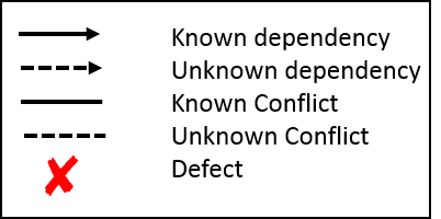
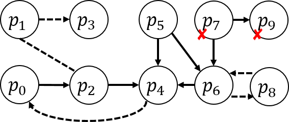
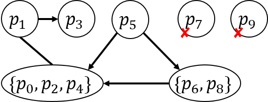
Full Learning: Given and bounds as above, return the mixed graph such that contains strongly connected components of all the packages, with the defective packages marked as such. are all the known and unknown conflicts between the nodes in , and are all known and unknown dependencies. A sample input and output of Full Learning is shown in Figure 3. Note that by solving Full Learning one gets an answer to Maximal Sub-repository as well.
The first objective is motivated by security updates, where one receives updates from multiple sources, that may depend on each other, conflict, or misbehave in the target system. Thus, we wish to find the largest possible subset of patches that can be safely installed, in order to make the system as secure as possible.
The second objective allows the system administrators to learn the exact state of the repository. As our main metric is the query complexity, a solution to this problem implies that we can also solve the first problem by local computation. Hence, this problem is the hardest and any lower bound on the first problem is directly applicable to it as well.
4 Learning when all dependencies are known
In this section, we assume that all the dependencies are known, no conflicts exist, but the repository may contain some root defects that could fail an installation. Specifically, we allow at most root defects, while there can be as many as defects overall.
Theorem 4.1
Denote ; any algorithm that solves group testing on items and at most defects requires queries.
Proof.
We start by observing that if there are no known dependencies (), the problem reduces to group testing over items and at most defects. Thus, the lower bound proven in [19] applies to our problem as well.
∎
We proceed with an algorithm for the case where , which is based on the Generalized Binary Splitting (GBS) method [16] mentioned above. Specifically, we show that its routine can be implemented despite the constraints imposed by the dependencies. We show that in this case, the number of tests required to learn the root defects and solve Full Learningadaptively is similar to that of group testing. Intuitively, the GBS algorithm arbitrarily chooses the sets to test while determining only their size. Here, we use the set of known dependencies to determine which packages to try at each point. In order to find a defect in a set of packages (for an ), we first compute a topological sort on its vertices [18], whereas the vertices with no outgoing dependencies have the highest indexes. That is possible as contains no cycles (as explained in Section 3.1). Then we first test the packages with the lowest indices in . If the test fails, we recurse on the tested vertices. Otherwise, we recurse on the remaining packages while adding the non-defective vertices to all future installations. That is, since we know that these packages are non-defective, we can safely add them to all other queries, thereby resolving dependencies of the other packages. Next, we follow a similar procedure for the main GBS iteration. Our algorithm starts by selecting the packages with the highest index in and thus ensures that they do not depend on other modules. If the test fails, we can use the above to find a defect using queries. Once a root defect has been identified, we remove all packages that depend on it as they are considered as defects. On the other hand, if the test succeeds, we repeat while adding these packages to future installations. Finally, if we can individually test each package according to their index in . Throughout the algorithm, we maintain the reservoir that for any two packages such that , is tested without only if is identified as a defect. Thus, we never test a package without installing all modules it depends on. We provide a pseudo code of our method in Algorithm 1.
Since in each test all dependencies are satisfied, and as we follow GBS at each iteration, we conclude the correctness and query complexity of our algorithm. This also proves the following theorem:
5 Learning with Unknown Dependencies
In the previous section, we assumed that all the dependencies are known and identified the defective packages. Here, we assume that some of the dependencies in the repository may not be documented. Thus, the GBS variant we proposed no longer works, and we need a different solution.
We now show that even if there exists no more than a single unknown dependency and a single root defect, no algorithm with a sub-linear number of queries exists even when adaptivity is allowed. Note that in this section we solve only Maximal Sub-repository. The more difficult problem, Full Learning, needs to be solved using algorithms presented in Section 7.
Theorem 5.1
Any adaptive algorithm that solves Maximal Sub-repository must make at least queries in presence of unknown dependencies and root defects.
Proof.
Denote and consider the directed path graph given by (as illustrated in Figure 4). Any installation considered by the algorithm is either a prefix of the line, i.e., for some , or an installation that does not take all of the prerequisites into consideration (and thus fails). In the former case, let us assume, by contradiction, that there exists an such that the installation was not tested by the algorithm. We use an adversary argument and show that the algorithm cannot distinguish between two problem instances with a distinct solution. For this, consider and assume that is a root defect, as illustrated in Figure 4 . The only installation that could work is , which the algorithm did not test. Thus, all queries made by the algorithm came back negative. There is no way for the algorithm to know whether the solution should be or which reflects the case where is a root defect. ∎

As shown in the theorem above, if we do not bound the number of defects, no algorithm can efficiently solve the problem even for a single root defect. Recall that a defect is a package that cannot be included in a successful installation. This can be either due to a bug in the package itself or due to a dependency on a corrupted package. Thus, we hereafter consider a bound on the number of defects. Intuitively, we will show that if is small, the problem becomes tractable again. Note that in Theorem 4.1 no bound was imposed on the number of defects, but rather on the quantity of root defects.
We proceed with a lower bound on the number of queries required by any non-adaptive algorithm when the number of defects is bound by . Recall that is the size of a as described in Section 2.3.
Theorem 5.2
Assume that the repository contains at most defects and unknown dependencies. Any non-adaptive algorithm for Maximal Sub-repository must make at least queries.
Proof.
Consider , i.e., a repository with no known dependencies. Assume that an algorithm tries less than installations before its output. Then there exists a pair of disjoint package-sets , of sizes and , such that no attempted installation includes all of and none of the packages in . We show that in this case, it cannot possibly find the maximal installation in the worst case. We denote and . The set of (unknown) dependencies is and the set of defects includes . An illustration of the setting appears in Figure 5.
Note that thus far . We now claim that the algorithm cannot possibly distinguish between the case where is a defect and the case where it is not. Notice that in order for to be a part of a successful installation, the installation must contain and none of the packages in . Thus, all installations attempted by the algorithm were either unsuccessful or did not contain . Since the same test results would be obtained regardless of whether is defective, we conclude that the algorithm cannot determine the maximal installation as it must contain if it is not defective. ∎

We now provide a non-adaptive algorithm for Maximal Sub-repository that requires queries. Notice that it is optimal up to the (-1) factor in the first parameter. We note that an algorithm for Full Learning is presented in the following section, but here we provide a more efficient algorithm for the simpler Maximal Sub-repository problem when no conflicts exist.
Intuitively, we construct a , factor in the known dependencies, and get a set of tests that will later allow us to infer the maximal installation. The improvement in query complexity over the Full Learning algorithm presented below is that when no conflicts exist, finding the maximal installation is equivalent to identifying defects.
Observation 1.
When no conflicts exist, the set of non-defective packages is the maximal installation.
Henceforth, we interchangeably refer to -sized binary vectors as subsets of . Fixing a canonical enumeration of , we say that the package is in a vector if its bit is set.. Formally, we construct a and define the test set as , where is defined as That is, given a vector we create a test that contains all packages whose bit is set, together with those that are prerequisites to some set-bit package. For example, if and then we test the installation . Notice that we can compute the transitive closure of the dependencies graph once in time and use it to compute in linear time for any vector .
After testing all installations, for all tests we receive a feedback of whether succeeded. We now prove that given we can identify all defects. First, for each package we define its set of successful installations.
Definition 1.
Given let be the set of tests that installed and be the installations that were successful.
We first show that a package is defective only if it was not successfully installed in any of the tests.
Lemma 1
A package is defective if and only if .
Proof.
Recall that by definition a package is defective if there exists no successful installation that contains it. Hence, immediately implies that . Our goal here is to show the converse – that implies that cannot be a part of any successful installation, including the ones that were not tested by the algorithm. Thus, we assume that , and show a test that was necessarily included in and succeeds.
We now construct disjoint sets of sizes and . Here, we choose to be the set of defects. Next, we define . In other words, we add to the package and every non-defective package that is a prerequisite to a package and the dependency was missing from . By adding to only non-defective packages we guarantee that as required. Also, we added at most packages to and at most packages to .22 2 We can add arbitrary packages to and to make their sizes exactly and if needed.
While we cannot determine and in advance, from ’s properties, we are guaranteed that there exists a vector such that and . Now, observe that if is not defective then must pass as it contains no defects and satisfies every dependency. The known dependencies are satisfied due to the propagation of in , and the unknown dependencies are satisfied as they are included in . Thus, we established that if is not defective then must pass as all defects were excluded and all dependencies satisfied. ∎
The pseudo code of our method for Maximal Sub-repository solution when no conflicts are present is given in Algorithm 2.
We conclude an upper bound on the non-adaptive query complexity of Maximal Sub-repository.
Theorem 5.3
Assume that the repository contains at most defects and unknown dependencies. There exists a non-adaptive algorithm that solves Maximal Sub-repository using queries.
Adaptive Algorithms Complexity
The method above is near-optimal with respect to non-adaptive algorithms. An important question is how much can we gain from adaptiveness in the test selection process.
We now show a lower bound of for adaptive algorithms. The gap from the query complexity of our non-adaptive algorithm is left as future work.
Theorem 5.4
Assume that the repository contains at most defects and unknown dependencies. Any adaptive algorithm for Maximal Sub-repository must make queries.
Proof.
First, note that a lower bound immediately follows from the group testing lower bound (as the case of degenerates to group testing). Fix an arbitrary package subset of size . Consider an algorithm that makes at most queries. Clearly, there are subsets of size of . Thus, there exists two disjoint-subsets pairs and such that and (also, ) and that no tested installation contains but none of and no test includes but none of . Consider the following scenarios:
- 1.
The set of defects is and all of the packages in depend on each other (i.e., there is a cycle that contains all of in ).
- 2.
The set of defects is and all of the packages in depend on each other (there is a cycle that contains all of in ).
Notice that in case I, any installation that contains but none of the packages in passes and similarly for case II and . As no such installations were tested by the algorithm, every test that contains at least one package of fails, regardless of the actual scenario. Thus, the algorithm cannot determine whether or belongs to the maximal installation and thus fails to solve the problem. ∎
6 Learning Conflicts when All Dependencies are Known
Previously, we assumed that the repository contained no conflicts, and identified the defects. In this section, we return to the case where all dependencies are known, but now the repository may have unreported conflicts. We start by showing that learning conflicts is “hard”, in the sense that even when all dependencies are known and no defects exist – identifying the exact conflicts requires a linear number of queries.
Theorem 6.1
Assume that all dependencies are known and no defects exist. Any non-adaptive algorithm that solves Full Learning must make at least queries. Note that this holds even when the repository may have only up to conflict.
Proof.
Consider the repository and the dependencies . If the algorithm makes queries or less, then there exists some , such that the algorithm does not query . In this case, the feedback for all the queries is the same in both case and case. Thus, the algorithm cannot determine which package is conflicting with and it fails to solve Full Learning. Similarly, if the algorithm does not attempt to install , it cannot distinguish between the case where the packages are in conflict with each other and the case where no conflicts exist. ∎
In order to “regain” the logarithmic query complexity, we consider a weaker notion of conflicts. For convenience, we also define the weak dependency notion. Intuitively, weakly depends on if there exist packages , such that .
Definition 2.
Given two packages , we say that weakly depends on if there exists no successful installation that includes but not . Also, weakly conflicts with if no successful installation includes both and .
Armed with the relaxed definition, we now analyze the query complexity of algorithms given bounds on the number of defects and weak conflicts. We start with a lower bound for Full Learning.
Theorem 6.2
Assume that the repository contains at most defects and unknown weak conflicts. Any non-adaptive algorithm that solves Full Learning must make at least queries.
Proof.
Assume by contradiction that the algorithm makes less than queries. This means that there exist a set and packages such that some tested installation contains and but none of ’s members. We will construct an input scenario for which Full Learning cannot be solved correctly by this algorithm. Consider the scenario where are defective packages and conflict with . This implies that no installation that contains and is tested. Thus, the algorithm cannot determine whether conflicts with or not.
The setting is depicted in Figure 6. Observe that the number of weak conflicts is at most as required and there are defects. Thus, the algorithm fails to solve Full Learning.

∎
We proceed with a non-adaptive algorithm for the Full Learning problem. The test selection is similar to that of the previous section. Namely, we construct a and propagate the known dependencies so that the tests are (see Section 5 for a formal definition of ). Following are lemmas that show that from the feedback we can infer all constraints.
Lemma 2
A package is defective if and only if .
Proof.
The claim is similar to Lemma 1 except that now we may have conflicts, and all the dependencies are known. Once again, if is defective, then clearly , and our goal is to show the converse. Given a non-defective , we construct sets of the required sizes such that a test containing all of and none of succeeds, thus showing that . Intuitively, we satisfy each conflict by excluding (having in ) one of its packages along with all those that depend on it. As for , all we need is to include as the dependency propagation will ensure that all its prerequisites are installed as well. The setting is illustrated in Figure 7.
Next, notice that if weakly conflicts with a prerequisite of itself, then cannot be successfully installed and is thus a defect. Hence, we hereafter assume that does not conflict with any of its prerequisites. We now formally define a pair of disjoint sets such that the corresponding test contains and passes. Here, . Next, we consider an arbitrary order on that will allow us to resolve the conflict constraints. We define two package sets as follows:
- •
.
- •
.
Intuitively, contains all packages that conflict with a prerequisite of ; ’s packages are those that have no relation to and have an unknown conflict with another package with a lower index (according to ). If we make sure that we have a test that installs all of ’s prerequisites and excludes all packages in , it will pass if is not defective. However, due to the propagation of the known dependencies, it is not enough to include just in . That is, if a package is a member of , but a package that depends on it has ‘‘ in the corresponding vector in the CFF, the propagation-result will include as well. We circumvent this issue by adding to all packages that weakly depend on , i.e., we set . Since every package in has an unknown weak conflict or defect we have that . Figure 7 illustrates the sets that allow the corresponding test to pass if is not defective.

Since we have and there exists a vector , such that and . By the construction of and we are guaranteed that the test includes and satisfies all conflict and dependency constrains. ∎
As mentioned, in the presence of conflicts, identifying all defects is not enough even for solving Maximal Sub-repository. We therefore show that our algorithm can also learn the conflicts themselves. Intuitively, if two packages weakly conflict, there exists no installation that contains both. Thus, we need to show that for every pair of non-conflicting packages our algorithm has a witness – a successful test that contains both.
Lemma 3
Packages weakly conflict if and only if .
Proof.
Notice that if weakly conflict then no test that contains both can pass and . In the remainder of the proof, we assume that the two do not conflict and show that the algorithm tries a successful installation that contains both. Similarly to the proof of Lemma 2, we define ; the resulting test will include and all their prerequisites. We also construct in a similar manner, where and
- •
- •
.
Observe that and . Thus, there exists such that and . Since the resulting test contains all of the prerequisites of and satisfies all other constraints, and since do not (weakly) conflict, this test passes.∎
Putting the lemmas together, we conclude that our algorithm can identify all defects and conflicts. The pseudocode for the algorithm is shown in Algorithm 3.
Theorem 6.3
Assume that the repository contains at most defects and weak conflicts. There exists a non-adaptive algorithm that solves Full Learning using queries.
6.1 Using Adaptivity to Reduce Complexity
The algorithm and lower bound presented above indicate a query dependency of on the number of defects. As the number of defects may be large, a natural question is whether this cubic dependency can be improved using adaptiveness. We now show that, indeed, adaptive algorithms have just a dependency on the number of defects.
Theorem 6.4
Assume that the repository contains at most defects and weak conflicts. There exists an adaptive algorithm that solves Full Learning using queries.
Proof.
The idea behind our algorithm is first to identify the defects, remove them from the repository and then follow the non-adaptive procedure when no defects exist. Recall that in the proof of Lemma 2, the size of was just one (only the package for which we wish to assert defectiveness). Hence, Lemma 2 also holds for . Therefore, by taking a and propagating the known dependencies, we can find all defects. The adaptivity then allows us to compute the subsequent only on the non-defective packages and learn all conflicts. ∎
7 Learning with Unknown Defects, Dependencies, and Conflicts
Heretofore, we considered cases where either unknown dependencies exist or unknown conflicts exist, but not both. In this section, we discuss the query complexity of the most difficult scenario in which the repository may have defects, hidden dependencies, and unknown conflicts.
We start by proving that learning unknown dependencies requires a linear number of queries if the number of known dependencies is not bounded, even if no conflicts or defects exist. This will lead us to bound the overall number of dependencies.
Theorem 7.1
Assume that no defects or conflicts exist. Any non-adaptive algorithm that solves Full Learning must make at least queries. Note that this holds even when the repository may have only up to 1 unknown dependency.
Proof.
Denote and consider the directed path graph given by . Assume by contradiction that there exists an algorithm that makes less than queries. In such case, there exists some , such that the installation was not tested. Next, consider two possible scenarios – and . That is, there is an undocumented dependency of either or on , as illustrated in Figure 8. The only way to distinguish between the two cases is to try the installation , as all other installations will result in the same outcome for both scenarios. Thus, the algorithm must try at least queries.

∎
To circumvent the problem above, we consider a bound on the overall number of dependencies in the repository. That is, we henceforward assume that there are at most unknown dependencies. Formally, we set and provide algorithms that learn all constraints without prior knowledge of the dependencies. An interesting implication of this assumption is that our upper bound now depends on the number of conflicts and not the, potentially larger, number of weak conflicts. Thus, the gap in query complexity might not be as large as it seems. We start with lower bounds where the first considers the maximal installation problem.
Theorem 7.2
Assume that the repository contains at most defects, unknown dependencies, and unknown weak conflicts. For the case that , any non-adaptive algorithm that solves Maximal Sub-repository must use at least queries.
Proof.
The setting for the proof is similar to that of Theorem 5.2 except that there are packages, each conflicting with one of , therefore they all indirectly conflict with . Another package directly conflicts with . Formally, if we assume that the algorithm tests less than installations, there exists a pair of package sets and such that no test contains all of but none of the packages in . In this case, we prove that the algorithm cannot determine whether is defective in the following scenario. Consider the dependencies , defects and conflicts . The setting is illustrated in Figure 9.

Notice that the number of dependencies is and that the number of weak conflicts is (as and are weak conflicts for ). As in Theorem 5.2, the algorithm has no way to distinguish between the case where is defective and the case that it is not, as no test that contains has passed. Finally, notice that the maximal installation contains and potentially , and thus the algorithm fails to solve the problem. ∎
Using a slightly different construction, we prove a stronger bound for the Full Learning problem.
Theorem 7.3
Assume that the repository contains at most defects, unknown dependencies and unknown weak conflicts. Any non-adaptive algorithm that solves Full Learning must use at least queries.
Proof.
Unlike the Maximal Sub-repository bound discussed earlier, an algorithm solving Full Learning must determine for every whether the two conflict. This allows us to consider the case where packages directly conflict with that also has unknown dependencies on , in addition to defective packages. The setting is depicted in Figure 10.

Observe that the number of unknown dependencies is , the number of defects is , and the number of weak conflicts is at most , as required. Since no installation that contains and excludes is tested, the algorithm cannot determine whether conflicts with or not, as the feedback for all other tests is identical for the two cases. ∎
We proceed with a non-adaptive algorithm for the Full Learning problem. The test selection is similar to that of the previous section, except that now we have no known dependencies to propagate. Namely, we construct a and the tests are simply . Following are lemmas that show that from the feedback of the tests we can infer all constraints.
Lemma 4
A package is defective if and only if .
Proof.
The difference between the model here and that of Lemma 2 is that we now allow unknown dependencies and assume that . As before, a defective package yields ; we show that if then we have a successful test that includes to witness that. Intuitively, we satisfy each conflict by excluding (having in ) one of its packages along with all those that depend on it. Unlike before, we split our unknown dependency resolution to cases. We wish to have all packages that weakly depends on active (i.e., in ). All other packages that have an unknown dependency are excluded (placed in ), and so are all the packages that depend on them. The setting is illustrated in Figure 11.
Next, notice that if weakly depends on two packages that conflict, then cannot be successfully installed and is thus a defect. Therefore, we hereafter assume that no two packages that weakly depends on conflict.
Following are formal definitions of sets such that the test that contains and avoids succeeds, thus serving as a witness to the non-defectiveness of . We define as and all of the the packages it depends on: . Once again, we consider some order on for resolving the conflicts. We define three package sets as follows:
- •
.
- •
.
- •
.
Intuitively, is the set of packages that have an unknown dependency and are not a prerequisite to . contains all packages that conflict with a prerequisite of . ’s packages are those that have no relation to and has an unknown conflict with another package with a lower index according to . If we make sure that we have a test that installs all of ’s prerequisites and excludes all packages in , it will pass unless is defective. Thus, we define .

Observe that every package in can be uniquely associated with a defect, conflict or dependency. Thus, we have and and hence there exists a vector (and subsequently, a test) such that and . By the construction of and we are guaranteed that the test includes and satisfies all conflict and dependency constrains. ∎
As mentioned, in the presence of conflicts, identifying all defects is not enough even for solving Maximal Sub-repository. We therefore show that our algorithm can also identify the dependencies and conflicts. As in the previous section, we show that if two packages do not conflict, then there exists a successful test that installs both and serves as a witness.
Lemma 5
Packages weakly conflict if and only if .
Proof.
Similarly to Lemma 3, a pair of conflicting packages cannot be included in a successful test. Here, we show that if no successful installation was tried by the algorithm, then such does not exist and the two packages conflict. In the remainder of the proof, we assume that the two do not conflict and show that the algorithm tries a successful installation that contains both. We define to include , and any of their unknown weak prerequisites. We also construct in a similar manner, where
- •
.
- •
.
- •
.
Observe that and that . Therefore, there exists a test such that and . The test contains all prerequisites of and satisfies all other constraints. Thus, it passes unless conflict. ∎
We are left with showing that the algorithm can also learn the unknown dependencies. If depends on , no test that contains but not can pass. We show that if no successful installation with and not is tested by the algorithm, then such does not exist and depends on .
Lemma 6
Package weakly depends on if and only if .
Proof.
As in the other lemmas, one direction here is straightforward – if weakly depends on then . We now construct sets , such that the corresponding test will include , exclude , and pass unless weakly depends on . This is achieved by excluding from the test , and all the packages that weakly depend on it, including and all its prerequisites, and resolving all unrelated conflicts, dependencies, and defects. Formally we set to include and all its prerequisites. We define , where:
- •
- •
- •
.
- •
.
In other words, excludes from the test all packages that weakly depend on ; removes all packages with unknown dependencies that are not a prerequisite to ; contains all packages that conflict with a prerequisite of ; and is the set of packages, chosen according to , that is used to resolve conflicts unrelated to . An illustration of the setting is depicted in Figure 12.

Observe that since , , we have . Finally, since we have that there exists a witness test that addresses all other constraints and passes unless weakly depends on . ∎
As our algorithm learns all missing constraints using the tests in , we conclude the following.
Corollary 1
Assume that the repository contains at most defects, unknown dependencies and conflicts. There exists a non-adaptive algorithm for Full Learning that uses queries.
Finally, we discuss a more careful test-design that allows us to reduce the number of queries needed.
Theorem 7.4
Assume that the repository contains at most defects, unknown dependencies and conflicts. There exists a non-adaptive algorithm for Full Learning that uses queries.
Proof.
Intuitively, our construction so far was wasteful in the sense that when a test needed to include , we added all its prerequisites to and added every other package with an unknown dependency into . While there can be at most prerequisites to , and at most other packages with a dependency, we have not used the fact that their sum is also bounded by . That is, assume that has prerequisites; then we add packages to and at most packages to . We can use this in the following way – we construct a set of Cover-Free Families such that is a . We then set the tests of the algorithm to be . Similar arguments to those of lemmas 4, 5, and 6 show that we still have witnesses for every non-defective package, every non-conflicting pair of packages and every non-dependent pair. The actual that the relevant test belongs to is the number of prerequisites of the package in the case of defectiveness and dependency-learning, and the total number of prerequisites of either or in the case of determining whether the two conflict. ∎
Adding Adaptiveness: As evident by the proofs of lemmas 4, 5, and 6, we can use a to learn all defects, a to learn the conflicts and a to learn the dependencies. Thus, we can start by learning all defects using queries for learning just the defects and then proceed with tests to determine the conflicts and dependencies. This allows us to shave a factor in the dependency on the number of defects. That can also be integrated with the union of argument presented in Theorem 7.4 to reduce the complexity further.
8 Related Work
Our work is related to the problem of software upgrades that has been widely studied by the community [20, 13, 1, 25, 26]. As many open source products such as Debian and Ubuntu operating systems are built from packages, some practical solutions for installing these products have been developed in the past. These solutions try to find a large subset of packages that are installable together. Most of them either use SAT solvers or pseudo-boolean optimizations [20, 13, 26] or develop greedy algorithms [1] to derive a solution to that problem, i.e., find an installable subset of packages that need to be installed (or upgraded). The Mancoosi [5] EU research project has been involved in solving the problem of open source packages distributions and organized competitions for finding SAT solver based solutions that maximize the number of installable package. As part of the project the authors of [22] investigated the capabilities of MILP solvers to handle the upgradeability problem and showed some improvements upon pseudo-boolean optimizations.
All of the aforementioned techniques assume that the dependencies and the conflicts are known and that the packages are indeed installable and do not contain defects. Our approach complements the existing techniques by learning the real structure of the dependencies graph.
Techniques for detecting bugs in software using tests is another related research area [21, 8, 23, 28]. They are used do discover an unknown number of bugs. However, since there are dependencies between packages in our problem, the combinatorial algorithms developed for detecting bugs may not be used directly and require adjustments.
Our choice of cover-free families for tests selection is based on its applications studied in [10, 17, 9, 11, 12, 27]. Hwang et. al. were the first to define cover-free families for non-adaptive group testing [17]. Their work has been followed by others that were using CFFs for group testing [9, 11].
Researchers also used cover-free families for finding an -simple -path [10] in a graph and solving cryptographic problems [12, 27].Our approach leverages the efficiency achieved by other researchers in computing CFFs [24, 7, 15], thus providing efficient algorithms for learning the entire relations graph representing packages in a software system.
9 Discussion
| Scenario | Adpt | Problem | Query Complexity Bounds | Thm # |
|---|---|---|---|---|
| At most root defects and no unknown dependencies or conflicts | ✓ | Full | Lower: | 4.1 |
| Learning | ||||
| Upper: | 4.2 | |||
| At most unknown dependency and root defect | ✓ | Maximal | Lower: | 5.1 |
| Sub- | ||||
| repository | ||||
| At most defects and unknown dependencies, no conflicts | ✗ | Lower: | 5.2 | |
| Maximal | ||||
| Sub- | Upper: | 5.3 | ||
| ✓ | repository | Lower: | 5.4 | |
| At most conflict and no defects or unknown dependencies | ✗ | Full | Lower: | 6.1 |
| Learning | ||||
| At most weak conflicts, defects and no unknown dependencies | ✗ | Lower: | 6.2 | |
| Full | ||||
| Learning | Upper: | 6.3 | ||
| ✓ | Upper: | 6.4 | ||
| At most unknown dependency and no conflicts or defects | ✗ | Full | Lower: | 7.1 |
| Learning | ||||
| At most unknown dependencies, conflicts, and defects. All dependencies are unknown | ✗ | Maximal | Lower: | 7.2 |
| Sub- | ||||
| repository | ||||
| Lower: | 7.3 | |||
| Full | ||||
| Learning | Upper: | 7.4 |
In this paper, we formalized a stylized model that allows us to reason about the complexity of learning undocumented software constraints in a given repository. We presented algorithms for four cases: where the entire dependencies structure is known, and we are interested in finding the defects; where we have up to unknown dependencies, and we wish to find all the defects and the dependencies; where we have up to unknown conflicts, and we wish to find all the defects and conflicts; and where up to dependencies and up to conflicts are unknown. We proved lower and upper bounds on the complexity of both adaptive algorithms for solving the problems of Full Learning and Maximal Sub-repository. Table 2 gives the summary of our results.
The first column in the table describes the scenario in which the algorithm is applied, the second states whether the algorithm is adaptive, while the third one states which problem is being solved. The fourth column states the query complexity bounds. There, we present the lower bound for all of the scenarios and problem variants. For the scenarios where the lower bound for query complexity was proved to be linear, we do not state the upper bound as it is at least linear. For simplicity of comparison between the different cases, we introduce the following notation. We say that is the asymptotic complexity for constant-many unknowns. Specifically, a function is in if it is in for some function . The upper and lower bounds for query complexity can then be presented using and notations for small , , and . The last column gives a reference to the theorem that proves the result. We note that the problems are easily solvable in , as all constraints are local. For example, to determine whether has an unknown dependency on we need to test with all its prerequisites and exclude and its dependents. As there are vertex pairs to test, this is doable in the mentioned query complexity. Alas, as is large and testing is costly, we wish to determine which scenarios are learnable in logarithmic complexity.
Our algorithms assume that there are no optional dependencies in the package repository for which we need to find a solution. This means that if a package a depends on b then any working installation that includes a must include b as well. However, for some package repositories, it might be the case that a depends on either b or c. Thus a working installation could be or , while will fail. In the future, we plan to investigate how our algorithms are affected by this definition of dependencies.
Another fundamental issue is setting the bounds on the number of unknown constraints. That is, we may not know in advance how many defects, hidden dependencies, or unknown conflicts exists in a repository. A possible workaround would be devising an anytime algorithm – an algorithm that has no predefined stopping condition but can generate output on demand. The natural operation for such an algorithm would be starting from small values for and incrementing them one at a time. The query complexity dependency on the parameters is such that the overall number of queries would not be much larger than if we had known the parameters to begin with. If the parameters, at the time of output, are not large enough to capture the actual number of unknown constraints then either the algorithms will fail to find a working installation or would mistake some packages as defective while in practice they are functional but with many unknown constraints.
References
- [1] Modelling and resolving software dependencies. https://people.debian.org/ dburrows/model.pdf (2005)
- [2] AptGet -Package management with APT. https://help.ubuntu.com/community/AptGet (2017)
- [3] Aptitude package manager. https://wiki.debian.org/Aptitude (2017)
- [4] Cupt package manager. https://wiki.debian.org/Cupt (2017)
- [5] The mancoosi project. http://mancoosi.org/papers/ (2017)
- [6] Smart package manager. https://labix.org/smart/ (2017)
- [7] Abdi, A.Z., Bshouty, N.H.: Lower bounds for cover-free families. The Electronic J. of Combinatorics (2016)
- [8] Aldaco, A., Colbourn, C., Syrotiuk, V.: Locating arrays: A new experimental design for screening complex engineered systems. In: Operating Systems Review (ACM). vol. 49, pp. 31–40. Association for Computing Machinery (1 2015)
- [9] Berger, T., Levenshtein, V.: Application of cover-free codes and combinatorial designs to two-stage testing. Electronic Notes in Discrete Mathematics 6, 518 – 527 (2001)
- [10] Bshouty, N.H., Gabizon, A.: Almost optimal cover-free families. In: CIAC. pp. 140–151 (2017)
- [11] Bush, K., Federer, W., Pesotan, H., Raghavarao, D.: New combinatorial designs and their applications to group testing. Journal of Statistical Planning and Inference 10(3), 335 – 343 (1984)
- [12] Chor, B., Fiat, A., Naor, M.: Tracing Traitors, pp. 257–270. Springer Berlin Heidelberg (1994)
- [13] Di Cosmo, R., Boender, J.: Using strong conflicts to detect quality issues in component-based complex systems. In: Proceedings of the 3rd India Software Engineering Conference. ISEC, ACM (2010)
- [14] Dorfman, R.: The detection of defective members of large populations. The Annals of Mathematical Statistics (1943)
- [15] Hajiabolhassan, H., Moazami, F.: Some new bounds for cover-free families through biclique covers. Discrete Math. (2012)
- [16] Hwang, F.K.: A method for detecting all defective members in a population by group testing. Journal of the American Statistical Association 67(339) (1972)
- [17] Hwang, F., Sós, V.: Non-adaptive hypergeometric group testing. Studia Sci. Math. Hungar 22 (1987)
- [18] Kahn, A.B.: Topological sorting of large networks. Commun. ACM 5 (Nov 1962)
- [19] Li, C.H.: A sequential method for screening experimental variables. Journal of the American Statistical Association (1962)
- [20] Mancinelli, F., Boender, J., di Cosmo, R., Vouillon, J., Durak, B., Leroy, X., Treinen, R.: Managing the complexity of large free and open source package-based software distributions. In: IEEE/ACM ASE (2006)
- [21] Martínez, C., Moura, L., Panario, D., Stevens, B.: Locating errors using elas, covering arrays, and adaptive testing algorithms. SIAM J. Discret. Math. 23(4), 1776–1799 (Dec 2009)
- [22] Michel, C., Rueher, M.: Handling software upgradeability problems with MILP solvers. In: LoCoCo (2010)
- [23] Segall, I., Tzoref-Brill, R.: Feedback-driven combinatorial test design and execution. In: Proceedings of the 8th ACM International Systems and Storage Conference. pp. 12:1–12:6. SYSTOR ’15, ACM, New York, NY, USA (2015), http://doi.acm.org/10.1145/2757667.2757677
- [24] Stinson, D.R., Wei, R., Zhu, L.: Some new bounds for cover-free families. J. of Comb. Theory (2000)
- [25] Trezentos, P., Lynce, I., Oliveira, A.L.: Apt-pbo: Solving the software dependency problem using pseudo-boolean optimization. In: IEEE/ACM ASE. pp. 427–436. ACM, New York, NY, USA (2010)
- [26] Tucker, C., Shuffelton, D., Jhala, R., Lerner, S.: Opium: Optimal package install/uninstall manager. In: Proceedings of the 29th International Conference on Software Engineering. pp. 178–188. ICSE ’07, IEEE Computer Society, Washington, DC, USA (2007), https://doi.org/10.1109/ICSE.2007.59
- [27] Yamada, S., Hanaoka, G., Kunihiro, N.: Two-Dimensional Representation of Cover Free Families and Its Applications: Short Signatures and More, pp. 260–277. Springer Berlin Heidelberg (2012)
- [28] Yilmaz, C., Dumlu, E., Cohen, M.B., Porter, A.: Reducing masking effects in combinatorialinteraction testing: A feedback drivenadaptive approach. IEEE Transactions on Software Engineering 40(1), 43–66 (Jan 2014)