Rational proofs for quantum computing

In this subsection, we propose our first protocol for BQP. Let us assume that the client wants to solve a decision problem $L$ in BQP. The client asks the server to solve the problem, and the server sends a single bit $b\in\{0,1\}$ to the client. If the server is honest, the server sends the client $b=1$ when the answer is yes $(x\in L)$, and $b=0$ when the answer is no $(x\notin L)$.

Since BQP is in PP, there exists a classical probabilistic polynomial-time algorithm $A$ that outputs $a\in\{0,1\}$ such that

• •

  If $x\in L$ then ${\rm Pr}[a=1]>\frac{1}{2}$.

• •

  If $x\notin L$ then ${\rm Pr}[a=1]<\frac{1}{2}$.

The client runs $A$. If $a=b$, the client gives the server the reward $\$=1$. If $a\neq b$, $\$=0$. The expectation value $\langle\$\rangle_{b}$ of server’s reward when the server sends $b\in\{0,1\}$ to the client is

Therefore, if $x\in L$,

If $x\notin L$,

This means that the rational sever wants to send the correct solution to the client.

Although we use the class PP, the important point here is that the server’s computational ability is enough to be BQP in our protocol. It is clear that the same proof holds for other classes in PP, such as AWPP, QCMA, QMA, SBQP, and ${\rm C}_{=}{\rm P}$, etc.

Let us explain our second protocol, which is for estimating output probability distributions of quantum computing. Consider an $n$-qubit quantum circuit $V$. Without loss of generality, we can assume that $V$ consists of only classical gates (such as $X$, CNOT, Toffoli, etc.) and Hadamard gates [32, 33]. (Generalizations to other gate sets, such as Clifford plus $T$, are given in Sec. IV.2.) Let

be the probability of obtaining $z\in\{0,1\}^{k}$ when the first $k$ qubits of $V|0^{n}\rangle$ is measured in the computational basis. We assume that $k=O(\log(n))$. The client wants to know a probability distribution $\tilde{p}\equiv\{\tilde{p}_{z}\}_{z\in\{0,1\}^{k}}$, which is close to $p\equiv\{p_{z}\}_{z\in\{0,1\}^{k}}$ in the sense that $|p_{z}-\tilde{p}_{z}|\leq\frac{1}{poly(n)}$ for all $z\in\{0,1\}^{k}$. Such an estimation $\tilde{p}$ can be obtained in quantum $poly(n)$ time (see Sec IV.3), but the client who is completely classical cannot do it by him/herself. The client therefore delegates the task to the server. We here provide a protocol where the client can receive such an estimation from the rational server.

From $V$, we construct the $(n+1)$-qubit quantum circuit

for each $z\in\{0,1\}^{k}$. It is easy to see

We can construct a classical probabilistic computing $M_{z}$ that “simulates” $W_{z}$ such that

where $h$ is the number of Hadamard gates in $V$, and $D_{z}(w)$ is the probability that $M_{z}$ outputs $w\in\{1,2,3\}$. In fact, Let $t$ be the number of elementary gates in $W_{z}$. In other words, $W_{z}=u_{t}\cdots u_{1},$ where $u_{i}$ ($i=1,2,...,t$) is a classical gate or the Hadamard gate. We consider the following $t$-step classical probabilistic computing $M_{z}$:

• 1.

  The state of the register is represented by the pair $(z,c)$ of an $(n+1)$-bit string $z\equiv(z_{1},...,z_{n+1})\in\{0,1\}^{n+1}$ and a single bit $c\in\{0,1\}$. The initial state of the register is $(z=0^{n+1},c=0)$.

• 2.

  For $i=1,2,...,t$, do the following:

  • 2-a.

    If $u_{i}$ is a classical gate, update the register as $(z,c)\to(u_{i}(z),c)$.

  • 2-b.

    If $u_{i}$ is the Hadamard gate acting on $j$th qubit, flip a fair coin. If heads, update the register as

    $\displaystyle(z,c)\to(z_{1},...,z_{j-1},0,z_{j+1},...,z_{n+1},c).$

    If tails, update the register as

    $\displaystyle~~~~~~(z,c)\to(z_{1},...,z_{j-1},1,z_{j+1},...,z_{n+1},c\oplus z_{j}).$

• 3.

  If the state of the register is $(0^{n+1},0)$, output 1. If the state of the register is $(0^{n+1},1)$, output 2. Otherwise, output 3.

An example of the computational tree for $n=2$, $t=4$, and

is given in Fig. 3.

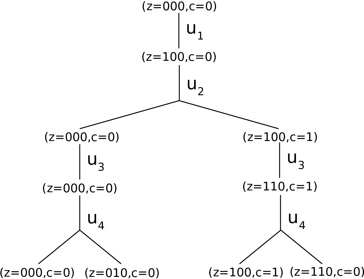
Now it is easy to check Eq. (2). (In the example of Fig. 3, $D_{z}(1)=\frac{1}{4}$, $D_{z}(2)=0$, and $D_{z}(3)=\frac{3}{4}$.) Therefore, from Eqs. (1) and (2), we obtain

Our protocol runs as follows.

• 1.

  The server sends a classical description of a probability distribution $p^{\prime}\equiv\{p_{z}^{\prime}\}_{z\in\{0,1\}^{k}}$ to the client. If the server is honest, $|p_{z}^{\prime}-p_{z}|\leq\frac{1}{poly(n)}$ for all $z$.

• 2.

  The client chooses $z\in\{0,1\}^{k}$ uniformly at random.

• 3.

  The client runs $M_{z}$ and obtains the output $w\in\{1,2,3\}$.

• 4.

  The client pays the reward to the server whose amount $\$$ is determined according to the following rule:

  • –

    If $w=1$, then $\$=S(z,p^{\prime})+2$.

  • –

    If $w=2$, then $\$=-S(z,p^{\prime})+2$.

  • –

    Otherwise, $\$=2$.

  Here,

  $\displaystyle S(z,p^{\prime})\equiv 2p^{\prime}_{z}-\sum_{\alpha\in\{0,1\}^{k}}(p^{\prime}_{\alpha})^{2}-1$

  is called Brier’s scoring rule [34].

The expectation value $\langle\$\rangle$ of the prover’s reward is

where we have used Eq. (3).

Note that

which means that $\langle\$\rangle$ is larger if $p^{\prime}$ is closer to $p$. As is explained in Sec. IV.3, the quantum polynomial-time prover can send $p^{\prime}$ such that $|p^{\prime}_{z}-p_{z}|\leq\frac{1}{poly(n)}$ for all $z$. If the server sends another $p^{\prime}$ such that $|p^{\prime}_{z}-p_{z}|=const.$ for a certain $z$, on the other hand, his/her expected profit becomes smaller. Therefore the rational prover will not do that.

Here we briefly summarize some of results in Ref. [31]. To understand the essence, let us consider the following protocol:

• 1.

  The client samples $w$ from a probability distribution $D$.

• 2.

  The server sends the client the description of a probability distribution $D^{\prime}$.

• 3.

  The client gives the server the reward $S(D^{\prime},w)$.

Here,

is called Brier’s scoring rule [34]. In the above protocol, server’s expected profit is $\sum_{w}D(w)S(D^{\prime},w).$ By the straightforward calculation,

Therefore, server’s expected profit is maximum when $D^{\prime}=D$. In other words, if the server wants to maximize the expected profit, he/she has to send $D^{\prime}=D$. The point is that this protocol enables the client, who can sample from $D$ but does not know the description of $D$, to learn the description of $D$ from the rational server.

In Ref. [31], this idea was used to construct a single-message rational protocol for $\#$P problems. Let

be a Boolean function that can be calculated in classical polynomial time. The client first samples an $n$-bit string $x\in\{0,1\}^{n}$ uniformly at random. He/She then outputs $\phi(x)$. The probability that the client outputs 0 is $\frac{\#\phi}{2^{n}}$, where $\#\phi$ is the number of $x\in\{0,1\}^{n}$ such that $\phi(x)=0$. In other words, the client can sample from the probability distribution

such that $D(0)=\frac{\#\phi}{2^{n}}$ and $D(1)=1-\frac{\#\phi}{2^{n}}$. The ability of sampling from $D$ is not enough for the BPP client to learn $\#\phi$, since the estimation of $D(0)$ with an exponential precision is required. However, if the client uses the above protocol, the client can learn $\#\phi$, since the rational server sends the client the description of $D^{\prime}$ such that $D^{\prime}(0)=\frac{\#\phi}{2^{n}}$ and $D^{\prime}(1)=1-\frac{\#\phi}{2^{n}}$.

Let us assume that a circuit $V$ consists of only Clifford and $T\equiv Z^{\frac{1}{4}}$ gates. In other words, $V=u_{t}\cdots u_{1}$, where $u_{i}$ ($i=1,2,...,t$) is $H$, $CZ$, $S=\sqrt{Z}$, or $T$. Let us consider the following $t$-step non-deterministic computing:

• 1.

  The state of the register is represented by $(p,c,k)$, where $p$ represents the tensor product of $n$ Pauli operators, $c\in\{+1,-1\}$ represents the sign, and $k$ is an integer that counts the number of non-deterministic transitions experienced. The initial state of the register is $(p=Z\otimes I^{\otimes n-1},c=+1,k=0)$.

• 2.

  For $i=1,2,...,t$, do the following:

  • 2-a.

    If $u_{i}$ is a Clifford gate $g$, update the register as $(p,c,k)\to(g^{\dagger}pg,c^{\prime},k)$.

  • 2-b.

    If $u_{i}$ is $T$ gate acting on $j$th qubit, and if $j$th Pauli operator of $p$ is $Z$, do nothing on the register.

  • 2-c.

    If $u_{i}$ is $T$ gate acting on $j$th qubit, and if $j$th Pauli operator of $p$ is $X$, do the following non-deterministic transition:

    $\displaystyle(p,c,k)\to\left\{\begin{array}[]{ll}(p_{1}\otimes...\otimes p_{j-1}\otimes X\otimes p_{j+1}\otimes...\otimes p_{n},c,k+1)\\ (p_{1}\otimes...\otimes p_{j-1}\otimes Y\otimes p_{j+1}\otimes...\otimes p_{n},c,k+1).\end{array}\right.$

  • 2-d.

    If $u_{i}$ is $T$ gate acting on $j$th qubit, and if $j$th Pauli operator of $p$ is $Y$, do the following non-deterministic transition:

    $\displaystyle(p,c,k)\to\left\{\begin{array}[]{ll}(p_{1}\otimes...\otimes p_{j-1}\otimes X\otimes p_{j+1}\otimes...\otimes p_{n},-c,k+1)\\ (p_{1}\otimes...\otimes p_{j-1}\otimes Y\otimes p_{j+1}\otimes...\otimes p_{n},c,k+1).\end{array}\right.$

An example for $n=3$, $t=6$, and

is given in Fig. 4.

It is easy to check that

where the summation is taken over all paths, $(p_{i},c_{i},k_{i})$ is the final state of the register corresponding to the path $i$, and

Hence

We generate $V|0^{n}\rangle$ and measure the first $k$ qubits in the computational basis. Output $X=1$ if the result is $z$. Otherwise, output $X=0$. We repeat it for $T$ times to correct $X_{1},...,X_{T}\in\{0,1\}$. If we define

it satisfies

due to the Chernoff-Hoeffding bound. If we take $\epsilon=\frac{1}{2^{k}n}$, $T=poly(n)$ is enough to guarantee that $|\eta_{z}-p_{z}|\leq\frac{1}{2^{k}n}$ except for an exponentially small probability. We do this procedure for all $z\in\{0,1\}^{k}$ to obtain $\{\eta_{z}\}_{z\in\{0,1\}^{k}}$. Except for an exponentially small probability, $|\eta_{z}-p_{z}|\leq\frac{1}{2^{k}n}$ for all $z$. Let us define

for each $z$. Then,

and

Therefore

for all $z$ except for an exponentially small probability.

Let $L$ be a language and $x$ be its instance. Assume that $L$ has the following rational proof system:

• 1.

  The server sends $b\in\{0,1\}^{m}$ to the client, where $m=poly(|x|)$.

• 2.

  The client samples a polynomial-length bit string $w$ from a probability distribution $D$, and sends the reward $\$(b,w)$ to the server.

• 3.

  The client calculates a predicate $\pi(x,b)\in\{0,1\}$ and accepts/rejects if $\pi(x,b)=1/0$, where $\pi$ is a polynomial-time computable Boolean function.

The expectation value of the server’s reward when he/she sends $b$ to the client is

We require that the rational proof system satisfies the following:

• •

  When $x\in L$ then there exists $b^{*}\in\{0,1\}^{m}$ such that $\pi(x,b^{*})=1$, and $\langle\$\rangle_{b^{*}}-\langle\$\rangle_{b}\geq\frac{1}{h}$ for all $b$ that satisfies $\pi(x,b)=0$, where $h=poly(|x|)$.

• •

  When $x\notin L$ then there exists $b^{*}\in\{0,1\}^{m}$ such that $\pi(x,b^{*})=0$, and $\langle\$\rangle_{b^{*}}-\langle\$\rangle_{b}\geq\frac{1}{h}$ for all $b$ that satisfies $\pi(x,b)=1$.

We can show that if $\max_{b,w}|\$(b,w)|\leq poly(|x|)$, then $L$ is in ${\rm NP}^{\rm MA[1]}$, which is in ${\rm NP}^{\rm MA}\subseteq\Sigma_{3}^{\rm P}$ [28]. It means that the above rational proof system will not contain BQP, because BQP is not believed to be in the third level of the polynomial-time hierarchy.

In fact, let us consider the following probabilistic polynomial-time algorithm $M$ on input $(x,b,a)\in\{0,1\}^{*}\times\{0,1\}^{m}\times\{0,1\}^{m}$:

• 1.

  Calculate $\pi(x,b),\pi(x,a)\in\{0,1\}$.

• 2.

  By using the Chernoff bound, calculate $\frac{1}{h^{2}}-$precision estimates, $\eta_{b}$ and $\eta_{a}$, of $\langle\$\rangle_{b}$ and $\langle\$\rangle_{a}$, respectively. Except for an exponentially small failure probability $e^{-poly(|x|)}$, $|\eta_{b}-\langle\$\rangle_{b}|\leq\frac{1}{h^{2}}$ and $|\eta_{a}-\langle\$\rangle_{a}|\leq\frac{1}{h^{2}}$.

• 3.

  If $\pi(x,b)=\pi(x,a)=1$, accept. If $\pi(x,b)=1$, $\pi(x,a)=0$, and $\eta_{b}-\eta_{a}\geq\frac{1}{h}-\frac{2}{h^{2}}$, accept. Otherwise, reject.

Then $L$ satisfies the following:

• •

  If $x\in L$ then there exists $b$ such that for all $a$, $M(x,b,a)$ accepts with probability at least $1-2^{-r}$, where $r=poly(|x|)$.

• •

  If $x\notin L$ then for all $b$ there exists $a$ such that $M(x,b,a)$ accepts with probability at most $2^{-r}$.

Therefore, $L$ is in ${\rm NP}^{\rm MA[1]}$.