Surface Topological Order and a new ’t Hooft Anomaly of Interaction Enabled 3+1D Fermion SPTs
Abstract
Symmetry protected topological (SPT) phases are well understood in the context of free fermions and in the context of interacting but essentially bosonic models. Recently it has been realized that intrinsically fermionic SPTs exist which only appear in interacting models. Here we show that the 3+1 dimensional realizations of these phases have surface states characterized by a new ’t Hooft anomaly, captured by a class. This is encoded in the anomalous action of symmetry on the surface states with topological order, which must necessarily permute the anyons. We discuss in detail an example with symmetry group . Using a network model of the surface we derive a candidate surface topological order given by a gauge theory. We relate our findings to anomalies valued in with various coefficients introduced previously in both bosonic and fermionic settings, and describe a general framework that unifies these various anomalies.
I Introduction.
In the last few years we have learned a lot about possible realization of symmetry in quantum systems. Symmetry protected topological phases (SPTs) have played an important role in this progress [1, 2, 3]. These are gapped states of matter protected by a symmetry : once the symmetry is broken, one can continuously connect an SPT phase to a trivial product state. Much of the interesting physics of SPT phases comes from their boundary, which must necessarily be non-trivial; the boundaries of 1+1 and 2+1 dimensional SPTs are either gapless or symmetry broken,[4] while in 3+1 and higher dimensions a new possibility exists: the boundary may be gapped and symmetry preserving at the cost of supporting intrinsic topological order.[5, 6, 7, 8, 9, 10, 11, 12] Moreover, in all cases the boundary of an SPT state is “anomalous”: the way it realizes the symmetry cannot be mimicked without the bulk. In fact, even though depending on the boundary dynamics different boundary phases may exist, all of these phases share a common anomaly that must match the bulk. For SPT phases of bosons a systematic understanding of this matching exists in several cases: i) projective symmetry on the boundary of a 1+1D SPT [13, 14, 15] ii) a CFT on the boundary of a 2+1D SPT [16, 17, 18]; iii) symmetric intrinsic topological order on the boundary of a 3+1D SPT - this is the case which will be of interest to us here.[12, 19]
How does one characterize a 2+1D intrinsic topological order in the presence of a global symmetry (also known as symmetry enriched topological order (SET))? In fact, a systematic algebraic theory of 2+1D SETs has recently been developed [20, 21, 22]. The following data goes into this theory: i) the anyon content and the braiding and fusion rules; ii) how the anyons are permuted under the action of the symmetry; iii) fractional quantum numbers carried by the anyons. It turns out that not all realizations of symmetry, which are seemingly consistent with anyon fusion and braiding can exist in a strictly 2+1D system. In particular, some assignments of anyon fractional quantum numbers cannot be realized in 2+1D [12]. The anomaly for a given symmetry fractionalization is given by an element , where is the symmetry group and is the -dimensional cohomology group with coefficients [23]. (Here and below, unless otherwise noted, we specialize to the case where is a unitary, discrete, internal symmetry.) A very physical interpretation of this anomaly exists: 3+1D SPT phases of bosons are also classified by , and it is believed that a 2+1D SET with anomaly can live on the surface of the corresponding 3+1D SPT. This belief is supported by a large class of examples.[12, 19]
In the discussion above we have glossed over the fact that an even more severe anomaly of the symmetry may be present. Namely, the permutation of the anyons under the action of the symmetry might itself be anomalous, even though it preserves the anyon fusion and braiding. This anomaly is measured by an element , where is the group of Abelian anyons in the topological order. Such anomalous 2+1D SETs cannot exist at the boundary of a 3+1D SPT, but may be interpreted in a certain way as living on the boundary of a 3+1D SET [24] (with the caveat that certain anyons are confined to endpoints of 3+1D loop-like excitations), or a 3+1D phase with higher form symmetry.[25, 26, 27]
One may ask, what is the corresponding situation for phases of fermions. While non-interacting SPTs of fermions to which the famous conventional topological insulators belong have been understood for some time now[28, 29, 30] and have in many ways precipitated the study of SPTs, the general classification of interacting fermion SPTs is fairly recent. The case of 3+1D fermion SPTs is particularly interesting since here for a unitary internal symmetry in the absence of interactions no non-trivial phases exist. Currently, general interacting fermion SPTs in 3+1D with symmetry are believed to be classified by three inputs [31, 32, 33]: a co-cycle and co-chains and satisfying certain algebraic conditions and modulo equivalence relations. For fixed , , solutions to these conditions differ by , which physically corresponds to stacking on a boson SPT phase. Thus, the intrinsically fermionic physics comes from the inputs and . The case gives so-called super-cohomology phases [34]: here, must be a co-cycle in . The case when the total symmetry group does not factor as is less well understood, although see Ref. 33 for an approach for Abelian via the classification of three loop braiding statistics.
What kind of surface topological order (STO) do 3+1D fermion SPTs admit? While many examples of such surface states have been constructed for topological insulators and superconductors protected by time-reversal symmetry (possibly in conjunction with other unitary symmetries),[10, 6, 7, 8, 9] no examples for the case of purely unitary symmetries are known. In fact, since for purely unitary internal symmetries the bulk is necessarily strongly interacting, here we don’t yet know any surface states, either gapless or topologically ordered. Our goal is to construct STOs for this case and to characterize the STO anomaly. We focus on bulk fermion SPTs in super-cohomology with symmetry group . We expect the corresponding surface topological order to possess a new anomaly characterized by a co-cycle . Indeed, we define such an anomaly for a general 2+1D fermion topological order. Again, the data that specifies the fermion SET is: i) the anyon content; ii) how the symmetry permutes the anyons; iii) the fractionalization of symmetry on the anyons. The new anomaly is associated with an obstruction to extending the symmetry fractionalization to fermion parity fluxes after gauging the symmetry. We construct a simple example of such an anomalous SET for symmetry group : the topological order is , i.e. a gauge theory together with the physical fermion . The subgroup acts on the anyons by a non-trivial permuation, and the anyons carry a particular fractionalization of . We conjecture that this topological order can live at the surface of a 3+1D fermion SPT. Indeed, for this symmetry, modulo bosonic SPTs, there is a single intrinsically fermionic super-cohomology phase corresponding to a non-trivial co-cycle .[31, 33, 35] We conjecture that the gauge theory above is a STO of this intrinsically fermionic SPT. In particular, we find that the anomaly co-cycle extracted from the topological order matches the bulk co-cycle. Further evidence in favor of our conjecture comes from a closely related example: a fermion crystalline SPT with symmetry group . Here, is an internal symmetry and is lattice translation symmetry along a particular direction. Such an SPT can be constructed by stacking layers of 2+1D fermion SPT with symmetry. The latter are classified by an integer [36, 37, 38]. We focus on the 3+1D crystalline SPT constructed by stacking layers with . As we will explain, this is a close cousin of the non-crystalline 3+1D super-cohomology SPT discussed above. For the crystalline SPT example, we can explicitly construct the STO by gapping out the gapless modes associated with the edges of the 2+1D layers. In this way, we obtain the gauge theory described above.
Having defined the anomaly for general 2+1D fermion SETs, we may ask, does this anomaly have a relation to the anomaly of bosonic SETs [24, 20]? Clearly, the two anomalies have a somewhat different physical interpretation: in the fermionic case the topological order can live on the surface of an SPT, while in the bosonic case it cannot. Furthermore, in the fermionic case we need to specify the fractionalization of the symmetry on the anyons, while in the bosonic case the anomaly appears already at the level of anyon permutation by the symmetry - i.e. no symmetry fractionalization is consistent with the anyon permutation. Nevertheless, the two anomalies can be united into a common framework that we introduce. One imagines a topological order where the permutation of the anyons by the symmetry is specified. Furthermore, a consistent symmetry fractionalization is specified for a subset of the anyons (closed under fusion). One then asks whether symmetry fractionalization can be extended to the rest of the anyons. The general anomaly is the obstruction to doing so. For the case of the original anomaly for bosonic SETs, the subset of anyons for which fractionalization is specified is just the identity particle (which carries no fractionalization). For the case of fermionic SETs, one may consider the modular extension of the topological order. The anyons of the original fermionic SET are the subset of the modular extension on which fractionalization is specified, the remaining anyons of the modular extension are the fermion parity fluxes, and one asks if fractionalization can be consistently defined on them. Other previously considered examples [39] also neatly fit into this general framework.
This paper is organized as follows. In section II, we review the properties of the 3+1D fermion SPT with symmetry and its cousin crystalline SPT with symmetry. We then introduce our proposed STO for these two SPTs in section III and give a physical argument why such an STO is anomalous. Section IV gives an explicit construction of the STO for the crystalline SPT. Section V gives a general definition of the anomaly class for 2+1D fermionic topological orders. In section VI, we apply this definition to our conjectured topological order for the SPT and show that the resulting surface anomaly class matches the bulk class. In section VII, we discuss the general framework for type anomalies in 2+1D topological orders. We conclude with some open questions in section VIII.
II 3+1D fermion SPT and its crystalline cousin.
In this section, we review some properties of the 3+1D fermion SPT with internal symmetry and explain how it is related to the crystalline fermion SPT with symmetry , where is an internal symmetry and is translation along a given direction.
A key role in our discussion will be played by 2+1D fermion SPTs with symmetry, so we review them first. Recall, these have a classification[36, 37, 38]. The phase with can be constructed by stacking a superconductor with constituent fermions charged under the symmetry and a superconductor with constituent fermions neutral under . The edge of the phase then consists of a right-moving Majorana fermion () charged under and a left-moving Majorana fermion neutral under . Likewise, the phase has right-moving Majoranas charged under and left-moving Majoranas neutral under . For even , we can group chiral Majoranas into chiral complex (Dirac) fermions ().
We now proceed to 3+1D. As already noted, in 3+1D modulo bosonic SPTs there is a single non-trivial fermionic SPT with internal symmetry .[31, 33] This phase is the generator () of a subgroup in the classification, where the phase is a bosonic SPT. There is also one other root bosonic SPT with this symmetry,[40] bringing the full classification to .[35] Here we focus on the intrinsically fermionic root phase. A physical picture of this phase consists of a soup of domain walls. Each such domain wall is decorated [41] with the 2+1D fermion SPT.
A key property of SPTs in both 2+1D and 3+1D is the braiding statistics of flux defects [3, 42, 40]. For SPT in 2+1D, we have[38]
| (1) |
Here, denotes the self-statistics of a flux defect , and denotes the full-braid mutual statistics of flux defects and . labels the generator of the symmetry and the generator of symmetry. (All quantities are given modulo and the extra factors of on the left-hand-side are necessary to eliminate the dependence coming from fusing a defect with point charges).
In 3+1D, the relevant process is the three loop braiding [42], i.e. braiding of two loops , linked with a third loop . For the intrinsically fermionic SPT, we have[33]
| (2) |
with all other braiding phases being trivial. Here is the self-statistics of loop linked with a base loop , and is the full-braid mutual statistics of loops , linked with a base loop . Furthermore, is the generator of , is the generator of , and is again the generator of . Focusing on the braiding of and fluxes in the presence of a base flux, we see that it exactly matches the braiding in the 2+1D SPT, Eq. (1). So we can think of the surface of flux loops as decorated with SPT; in particular, the loop traps gapless modes, which coincide with those of the SPT edge. Here is another consequence of the above braiding statistics: let us compactify the system on a spatial manifold , where is a two-dimensional manifold. We can view the whole system as a 2+1D SPT with symmetry. Then switching the flux along from to changes the 2+1D SPT index by .
We now proceed to describe the closely related 3+1D crystalline SPT protected by symmetry. We choose to be translation by lattice constant along the direction. We build the phase by stacking along the direction layers of 2+1D SPT lying in the plane, see figure 1. This clearly defines a non-trivial crystalline SPT. Indeed, let us make the direction periodic. For the length of the direction large, but finite, we can think of the system as being effectively two-dimensional lying in the plane. Then changing the number of layers (i.e. the length of the direction) by one changes the SPT index of this two-dimensional system by . This means that the crystalline SPT is non-trivial. For instance, the surfaces possessing translational symmetry along the direction (e.g. the surface) cannot be trivially gapped, since for they are effectively the edge of a non-trivial 2+1D SPT. Now, there is an evident similarity to the SPT described above, where inserting a flux along a cycle resulted in . For the present crystalline SPT the same occurs when we change . But for translational symmetry, changing the length of the system by is, indeed, the definition of inserting a flux. So the crystalline SPT behaves like the internal symmetry SPT above with . A slightly more physical way to think about the same issue is to consider “flux defects” of the translational symmetry , i.e. the dislocations. These correspond to one of the layers terminating prematurely in the bulk - thus, the dislocation obviously carries the edge-modes of a 2+1D SPT - see figure 2.
III Surface topological order for SPT.
Here we briefly describe our conjecture for the STO of the 3+1D SPT. For the crystalline SPT, we will explicitly construct such a STO termination in section IV. In the present section, we will give a physical argument why such a topological order is anomalous both for the case of internal and crystalline symmetries.
Our proposed STO has anyon content . The first factor is a gauge theory ( version of the toric code). The second factor contains only one non-trivial particle - the physical fermion . We remind the reader that the gauge theory is generated by Abelian anyons and , where and are both self-bosons, and the full-braid mutual statistics . Further, .
The anomaly of the STO comes from the combination of anyon permutation under the symmetry and the fractional quantum number assignments. We take the symmetry not to permute the anyons, while the generator of acts as:
| (3) |
It is easy to check that this permutation preserves the fusion and braiding rules. Next, we specify the symmetry fractionalization on the anyons. We take to carry charge under , while carries no fractional charge under . Schematically, we write,
| (4) |
Note that we have not specified the fractionalization data for the symmetry here. This data will be discussed in section VI and explicitly derived for the crystalline SPT (with ) in section IV. For the crystalline SPT our proposed STO has the same anyon content and symmetry data (3), (4), with the replacement .
We now argue that the topological order with the symmetry action above is anomalous, i.e. it cannot exist strictly in 2+1D. To see this, imagine introducing flux defects of the symmetry. By potentially pasting on superconductors and SPTs, we can ensure that the flux defects are Abelian11 1 Indeed, consider the topological order with the fermion parity gauged. There are 16 such modular extensions, corresponding to the 16 modular extensions of . By pasting on a suitable number of symmetric superconductors (e.g. constructed from fermions neutral under ) we can ensure that the modular extension is the toric code , with , - the fermion parity fluxes. Since the original anyons are not permuted by , consistency with fusion/braiding requires that under either or . In the second case, we can paste on an SPT. When the fermion parity in such an SPT is gauged, one gets the toric code with . So, pasting on this SPT makes and under . Then none of the anyons in the modular extension are permuted by , which means that the defect must be Abelian.. We can think of the symmetry action on as arising from braiding around , i.e. such a process results in a Berry phase . Similarly, braiding around should give no Berry phase. Now, since is a flux, fusing should give one of the original anyons in the theory. But braiding with should give Berry phase and braiding with should have given Berry phase . The only anyons with the right braiding properties are and , i.e. or . Let us focus on the case , the argument for is identical. Now, under the action the flux defect can transform to a different flux defect . All the flux defects have to be related by fusion with an anyon in the original theory, so for some . Now, for consistency of symmetry with fusion , which means that . But there is no anyon in which fuses with itself to . So we’ve arrived at a contradiction and the topological order is anomalous.
We note that the above argument for the anomaly would likewise go through if the internal symmetry is replaced by the translation symmetry. Indeed, we have not attempted to introduce defects of symmetry anywhere in the argument and only used its global action.
IV Surface topological order for the crystalline fermion SPT.
In this section we explicitly construct the STO discussed above on the surface of the 3+1D crystalline fermion SPT. We start with the “stack” model of the crystalline SPT (figure 1) discussed in section II. Consider e.g. the surface of the stack: it consists of an array of 1+1D gapless SPT edges. Our goal is to gap out these edges without breaking the symmetry. Let us decorate the surface with strips of topological order arranged periodically, see figure 3 (top).
We choose the symmetry to act on this topological order as in Eq. (4). We would like to “stitch” the strips of topological order together and in the process gap out the SPT edges. To understand why this stitching works, we can focus on a single T-junction on the surface and perform the following thought experiment: imagine “bending” the SPT layer onto the surface, figure 3 (bottom). On the right of the junction we then have the topological order and on the left - the same topological order stacked with a SPT. Now, we make a key claim: the topological order can “absorb” the SPT, i.e. the state on the right of the junction and the state on the left of the junction are identical as SETs. Therefore, the two can be stitched together without breaking the symmetry. Performing this stitching on the entire array of T-junctions we obtain the desired STO.
We now elaborate on the above steps.
Absorbing the SPT
Let us show that the gauge theory with action (4) can absorb a SPT. Here, we imagine a purely 2+1D setting with a 1+1D edge (left side of figure 3, bottom). Recall, the edge of the SPT admits a Luttinger liquid description:
| (5) |
where is the electron. We drop kinetic energy terms of form here and below. Likewise, we can describe the edge of the gauge theory by:
| (6) |
where is the particle, and - the particle. Under ,
| (7) |
with and unaffected. Combining the STO edge and the SPT edge,
| (8) |
where ,
| (9) |
and
| (10) |
Now, consider a change of variables
| (11) |
We have and . This means that , is a symmetry of the topological order (we use the superscript to differentiate it from the original symmetry). However, in our edge construction, does not commute with the symmetry (7)22 2 This is the first hint that the transformation has a mixed anomaly with the symmetry.. In fact,
| (12) |
The transformation is a pure gauge rotation, so can be ignored. Thus,
| (13) |
This is the same as in our original topological order, but without the extra SPT on top. Indeed, the extra , modes can be gapped out by
| (14) |
When written in the primed variables it is especially clear that this gapping process does not break the symmetry. This proves that the gauge theory can absorb the SPT.
Stitching.

We are now ready to stitch the strips of topological order in figure 3 (top) together and eliminate the gapless SPT modes. A top view of our construction is shown in figure 4. The array of gapless modes coming from the SPTs is described by:
| (15) |
where labels the coordinate of the mode, . Under translations,
| (16) |
and under ,
| (17) |
The strips of topological order are described by:
| (18) |
The unbarred and barred variables correspond to right and left edges of the topological order strips, i.e. live at , and at . As before, the charge assignments are
| (19) |
and translations act by shifting the index .
If we focus on all the modes at , we have
| (20) |
Following the discussion in the previous section, we consider the gapping term,
| (21) | ||||
| (22) |
where as before , Eq. (11). The terms above gap out all modes at , as is especially clear in the primed variables, Eq. (21). Furthermore, they effectively glue , . This means that both the and particles can move across the “seams” at , i.e. the surface as a whole forms a single topological order. To label the topological charges globally, we will use, say, the strip as the reference point, so is . Since in the topological sense, any is in the sector.
action.
Now, let us investigate the action of symmetry on the above STO. The particle carries charge throughout. The particle carries no fractional charge. Under translation,
| (23) | ||||
| (24) |
This is exactly the action (3).
For topological orders with a combination of an internal symmetry ( in our case) and translation there is one other piece of data that characterizes the symmetry fractionalization: whether the action of and commutes on the anyons. Generally, on an anyon for some phase , where and is a translation by lattice sites. To extract the phases we follow the procedure of Ref. 45. Imagine a state with an anyon at position (there is another anyon at that goes along for the ride). Under translation by , where is a string operator that moves from to . Crucially, we assume here that preserves the anyon type, (otherwise, the string operator does not exist). By computing the charge of under , we find if and commute or anti-commute on . Let’s implement this procedure. We begin with the anyon . We have,
| (25) |
with . Here we used the fact that due to the gapping terms, . is neutral under , so and commute on . Now, does not preserve anyon type under translation by , however, does. We have,
| (26) |
with . is odd under , so and anti-commute on . Finally, we observe that while is not invariant under , it is invariant under . We have
| (27) |
with
| (28) |
is odd under , so and anticommute on .
We summarize the above data in table 1.
Let us describe an intuitive understanding of the origin of the anyon permuting symmetry. Our aim is to stitch together the adjacent topological orders at the bottom of Figure 3. Maintaining symmetry implies that the corresponding symmetry flux can freely tunnel across the interface. Let the symmetry flux on the right half be called : this is a boson which satisfies so that the -particles of the topological order carry charge . Next, let us call the symmetry flux on the left side of the junction . The key observation is that on passing through the fermion SPT layer, the symmetry flux acquires a topological spin of . Thus is a fermion, and the only consistent assignment is . For the symmetry fluxes to smoothly tunnel across the junction, we need to condense on the boundary, which is disallowed due to the mismatch in topological spin. To rectify this, there is a different combination using the modified flux: , which allows for a condensate of on the boundary. This implies the square is also condensed, which from the previous relations tells us that . This clarifies why a topological order is required (and a simpler toric code order would not suffice). Also note, this phenomenon of symmetry permuting anyons is not necessarily required for STOs of boson SPTs. For instance, take the “double,” , of the presently considered fermionic SPT. We would use the SPT in the stack construction, which is essentially bosonic. Now the topological spin of the flux defect changes only by , which is not visible on considering .
Before we conclude this section we note that there is a simple generalization of the bulk SPT and surface STO discussed here to the case when the symmetry is enlarged to a full particle-number symmetry. We discuss this generalization in appendix A. A nice feature of the case with the symmetry is that the projective transformation of under on the surface is closely linked to the identical projective transformation of the monopole in the crystalline SPT bulk. In addition, this gives us a promising direction to the physical realization of this crystalline SPT state. The symmetries required are charge conservation, i.e. , a translation symmetry and an additional internal symmetry. Furthermore, time reversal must be broken as in a magnetic insulator. Finally we note that the symmetry cannot be lifted to a second translation symmetry, since the symmetry fractionalization relies on the finiteness of this part of the symmetry group.
V General anomaly matching condition for super-cohomology fermionic SPTs with onsite symmetries.
We now describe a general anomaly matching condition between bulk fermionic SPT orders and topologically ordered surface states, at an algebraic level.
V.1 Bulk fermionic SPT order
First, let us recall the classification of 3+1D fermionic SPTs with symmetry group proposed in Refs. [31, 32]. Modulo stacking bosonic SPTs, such fermionic SPTs are classified by -valued functions and satisfying the properties:
| (29) | |||
| (30) |
This data is also subject to the following redundancy conditions:
| (31) | ||||
| (32) |
For a definition of the cup product, higher cup product, and the derivative , see e.g. Ref. [31]. There is a further condition on , , which in the simplest case reads as a cohomology class in .[32, 31]
Phases with non-trivial can be visualized in the following way. As with all symmetric phases, we can think of the ground state as a soup of domain-walls of . Consider a 1d junction of three domain walls corresponding to elements , and . If , such a junction traps a Kitaev chain. Phases with non-zero are called ‘beyond super-cohomology’ phases, and are not going to be the focus of this paper, although we will briefly speculate about the surface topological orders that they can support in the next subsection.
The super-cohomology phases, i.e. the ones with , will be the focus of this paper. In this case, itself can be taken to be by performing the appropriate gauge transformation. The above data then just reduces to a cohomology class - this is the bulk SPT invariant that we will try to match onto a surface anomaly.
V.2 Surface topological orders and symmetry
A 2+1D topologically ordered surface in the fermionic setting is described by a spin-TQFT, or, algebraically, a unitary pre-modular category with a single transparent particle , the local fermion. Each such has a modular completion, i.e. a larger unitary modular tensor category
| (33) |
where . Here the particles in are the fermion parity -fluxes, which all have non-trivial braiding with the fundamental fermion .
Now, a symmetry action of on such a unitary pre-modular category is described, at the coarsest level, as a map from to the braided auto-equivalence group of . A braided auto-equivalence of is roughly just a permutation of the anyons in , , that is compatible with the braiding and fusion structure. Formally, it is defined by also specifying unitary linear maps on all of the fusion spaces,
| (34) |
where is a unitary matrix. The braided auto-equivalence is only defined up to natural isomorphisms , such that ,
| (35) |
where are phases. Thus, to each element we assign a braided auto-equivalence . We will alternatingly use the notation . The group-law must be satisfied up to a natural isomorphism:
| (36) |
where
| (37) |
In the remainder of this section we will for simplicity only focus on the situation for all , in which case can all be taken to be as well. This is sufficient to describe all the examples we present, and we believe that the more general situation with non-trivial can be handled with a slight extension of our formalism, see in particular section VII. For more information on braided auto-equivalences see Refs. 20, 23, 22.
In the ‘beyond cohomology’ situation , we conjecture that, although acts on by braided auto-equivalences, these cannot be extended to braided auto-equivalences of its modular completion in a way consistent with the group law. Conversely, in the super-cohomology situation we believe that the action by braided auto-equivalences can always be extended to the modular completion . Let us now focus exclusively on this super-cohomology situation.
Given a valid action of by braided auto-equivalences, we can define another piece of data that characterizes the action of symmetry on the anyons, namely the symmetry fractionalization data. In the case when does not permute the anyons at all - i.e. trivial braided-auto-equivalence action - such fractionalization data amounts to an assignment of a projective representation of to each anyon ,
| (38) |
where are phase factors satisfying the usual co-cycle condition . In the case of anyon-permuting symmetries, we can argue, using physical considerations similar to those of Ref. 20, that at the surface of a fermionic SPT the fractionalization data should still be encoded in a set of phases satisfying now the twisted co-cycle condition:
| (39) |
as well as
| (40) |
for any in the fusion product of and . This is analogous to Eq. 164 of Ref. 20, where we have made use of our assumption to simplify the left hand side. We will make an extra assumption that - indeed, the particle is a local excitation, so it does not transform projectively under the symmetry.
As in the bosonic case, the next step is to argue that we can represent this fractionalization data equally well as a collection of Abelian anyons satisfying
| (41) |
with the monodromy for the exchange of and . When one of and is an Abelian anyon, is a pure phase - the full-braid exchange statistics. We refer the reader to appendix B for a proof that satisfying (41) always exists. is not unique: rather, it is only unique up to fusion with the transparent fermion . Also, from Eq. 39 we see that the anyon
| (42) |
must have trivial braiding with all other anyons, i.e.
| (43) |
Now, because was well defined only up to fusion with , we see from Eq. 42 that is also well defined only up to the differential of a -co-chain valued in . Furthermore, it is clear that . Thus, we have a well-defined cohomology class .
The crucial point is that might be non-zero. Indeed, despite the fact that , it might be impossible to write as the differential of something -valued. In this case (), one cannot extend the fractionalization class to a valid fractionalization class in the modular completion of , since such an extension is precisely a solution to
| (44) |
where differs from at most by a fermion . Here we have assumed for simplicity that in the modular completion ; again, this is true in the examples we consider, and our argument can presumably be generalized to the case of non-trivial in the modular completion.
Thus, a non-trivial signals an anomaly and shows that the bulk fermionic SPT order is non-trivial. The natural conjecture is that the bulk SPT order is also described by the same cohomology class . Although we do not prove this conjecture in general, in the next section we will compute for the STO derived in the previous section for and show that it indeed matches the bulk SPT order.
We note that a non-trivial is only possible if the symmetry permutes the anyons. Indeed, we can always write the group of Abelian anyons , as , where is a subgroup of . We can make a gauge choice where for all , . If the symmetry does not permute anyons then , which implies .
VI Example: surface topological order for SPT.
We now apply the formalism of the previous section to the conjectured STO of the SPT discussed in sections III, IV. The STO is a gauge theory times a trivial fermionic theory , with particles , , . We will refer to this fermionic topological order as . As discussed in the previous section, since we are at the surface of a fermionic SPT, we can specify the symmetry action at the level of braided auto-equivalence and fractionalization class , with - the group of Abelian anyons. We now describe these in detail.
VI.1 Braided auto-equivalence action
For a group element we will use the notation , , . Similarly, we will represent an anyon as :
| (45) |
A group element induces the following permutation action:
| (46) |
Note that the permutation action of the generator is trivial.
At the level of splitting spaces we define
| (47) |
to act by the phase factor
| (48) |
where denotes the largest integer smaller or equal than . To see that these are valid braided auto-equivalences, we really only have to check the case , as arise from taking powers of the case . In particular, the natural equivalences in Eq. (36) are all identically equal to .
So we just have to check that with is a valid braided auto-equivalence, i.e. that it commutes with all of the and symbols. The symbols are all trivial in this theory, and therefore commute with because is a multiplicative bilinear form on . Checking that commutes with the symbols requires a computation. First, we have
| (49) |
and therefore
| (50) |
commuting with the symbols means
It is easy to show that the braided auto-equivalence action extends to a modular completion of this fermionic theory. Indeed, one modular completion of the trivial fermionic theory is just the toric code, so for the modular completion of we can just take the theory equal to a gauge theory times a gauge theory.
For quasiparticles of we will use the notation , , . Here is the fundamental fermion , and odd corresponds to the -flux sector. Again, the braided auto-equivalence action of depends only on :
| (53) |
At the level of splitting spaces we define
| (54) |
to act by the phase factor
| (55) |
Just as before, one can explicitly check that this commutes with all the and symbols, and that all of the natural isomorphisms are trivial.
VI.2 Fractionalization class
In the previous subsection we specified the action of symmetry by braided auto-equivalences, and found that all of the , both in the fermionic theory and in its modular extension . Now we want to specify the symmetry fractionalization. This amounts to specifying a function from to the anyons with the property that for all .
Define:
| (56) |
Here and below we let if is even and if is odd. Let us calculate , using Eq. 42.
| (57) | ||||
| (58) | ||||
| (59) | ||||
| (60) |
A short calculation, utilizing the identity , gives:
| (61) | ||||
| (62) |
i.e. is valued in . It is easy to see that is non-zero. Indeed, it is the product of the generator of with the generator of in the cohomology ring, which is just a tensor product of the individual cohomology rings of and . This is the same cohomology class that describes the bulk SPT order for in Ref. 33.
VI.3 Relation to the topological order constructed for the crystalline SPT
Let us compare the topological order we formally described in sections VI.1,VI.2 to one constructed on the surface of the crystalline SPT in section IV. First, it is believed that for SETs with translation symmetry, one may formally treat translations as an internal symmetry for the purpose of specifying the symmetry data.[45] Observe that the (46), (48) and (56) are still consistent if we replace . Furthermore, is still a non-trivial co-cycle in . Now, this is actually the same STO as constructed in section IV. Indeed, it has the same quasiparticles and the same permutation action of the symmetry. It remains to check that it has the same fractionalization data, table 1.
Recall, for anyon which is not permuted by symmetry elements and , the projective action of the symmetry on is given by Eqs. (38), (41). From Eq. 56 we have , with and . In particular, , so and . This agrees with carrying charge under and carrying no fractional charge. Next, we proceed to the “commutator” of and . We have . Now, , , . Therefore, the commutator of and on is - trivial, and on , - in agreement with table 1. Finally, , , , so the commutator of and on is , again in agreement with table 1.
VI.4 STO
We now perform one more check on our STO for the SPT. Two copies, , of this fermion SPT give rise to a purely bosonic SPT, as can be checked e.g. from the three-loop braiding data in Eq. (2). Indeed, by doubling the phases in (2), we see that the state will be characterized by
| (63) |
with all the other braiding invariants being trivial. But this is precisely the braiding data of a bosonic SPT with symmetry corresponding to a co-cycle with
| (64) |
see Ref. 40. Let us confirm that this is consistent with the STO we’ve constructed for the phase.
If we stack two copies of the STO, we get a theory with topological order with the first two factors generated by (, ) and (, ) respectively. The symmetry transformations are inherited from each STO copy, . Likewise, the projective factors are inherited from each copy, so that the class is
| (65) |
It is easy to check that now , i.e. there is no anomaly. This suggests that we are dealing with the surface of a bosonic SPT. We would like to find out if this SPT is trivial or not. To do so, it is convenient to first simplify the STO by driving an anyon condensation transition. Let us condense the anyon . After eliminating the confined anyons and performing anyon identification, we are left with a topological order generated by , and . Note that the condensing anyon is not permuted by the symmetry and carries a trivial fractionalization . Thus, the condensation does not break the symmetry. After the condensation none of the anyons are permuted by the symmetry since now . The fractionalization class (65) now becomes
| (66) |
i.e. carries charge under , and , anticommute on . Clearly, the fermion now plays no role in the resulting topological order and symmetry action, so this is an STO of a bosonic SPT. Since the anyons are not permuted by the symmetry, we can use the result of Ref. 12 to compute the co-cycle characterizing the bulk bosonic SPT:
Now, in the gauge theory all the symbols are trivial, so using , we, indeed, reproduce Eq. (64).
VII General obstruction
In this section we describe a general formalism that unites the anomaly introduced in this paper with other anomalies introduced in other contexts. Let be braided fusion categories and a finite unitary symmetry group. Suppose for now that is modular, although later we will generalize beyond this. Suppose we have an action of by braided auto-equivalences on , and that is preserved under this action, so that there is an induced action by braided auto-equivalences on . Let and denote the Abelian groups of Abelian anyons in and respectively; in particular . Suppose that there is no obstruction to localizing the symmetry on and defining a symmetry fractionalization class for those anyons. One can then ask: what is the obstruction to extending this fractionalization class to all of ? We will see that in general it is valued in , where is the subgroup of consisting of Abelian anyons that have trivial braiding with (there is an additional mild technical assumption that we spell out below).
Before we give the argument, note that several different examples given in the literature are special cases of this obstruction.
(1) If we choose to be the trivial category, then , and the obstruction is valued in ; this is just the original obstruction of Ref. 23.
(2) If is a fermionic theory and its modular completion, then and we have the obstruction given in this paper.
(3) Let be a gauge theory with non-trivial Dijkgraaf-Witten twist, so that its anyons form the group under fusion. It is natural to label the generator of this as . Then let be the subgroup of gauge charges , where we have defined . Then Ref. 39 shows that certain extensions of the gauge group by the symmetry group are inconsistent with the twist. But this extension data just specifies a fractionalization class of on , for a trivial braided autoequivalence action on and . Hence according to our general result this inconsistency is encoded in , since .
Returning to the general formalism, to derive our obstruction, start with the natural isomorphisms defined in Eq. (36). These restrict to natural isomorphisms on . The action of on splitting spaces can be decomposed into factors , see Eq. (37), from which one constructs
| (67) |
and finds that
| (68) |
where is an Abelian anyon.
Now suppose that, when restricted to the anyons in , the symmetry can be localized. Precisely stated, this assumption means that one can find phase factors , , satisfying whenever , such that
| (69) |
for all . The question we want to ask is: given , what is the obstruction to extending them to a full set of satisfying whenever ? In essence, given a choice of symmetry localization on , what is the obstruction to extending it to all of ?
To answer this question, we first have to make a technical assumption: we assume there exist Abelian anyons such that
| (70) |
for all . Certainly this assumption holds for Abelian theories . Also, there definitely exist non-Abelian theories where this assumption fails for some such multiplicative functions (e.g. ). In any case, assuming the existence of , it is clear that it is well defined up to fusion with anyons in , where is the subset of Abelian anyons which have trivial braiding with .
Define now
| (71) |
Then has the key property that its braiding with any anyon in is trivial. Hence . Finally, note that is clearly a co-cycle, and since is ambiguous up to fusion with anyons in , is only well defined up to the co-boundary of a -valued -co-chain. Hence determines a cohomology class
| (72) |
VII.1 Special case
In the special case where the braided auto-equivalence action on has no obstruction, we can make the above discussion slightly more concrete. In this case we can find decomposition factors for which vanishes identically. Then a choice of symmetry localization on is precisely a choice of phase factors , , satisfying whenever , such that
| (73) |
for all . Again, we want to ask: what is the obstruction to extending to all of ? To answer this, we again make the technical assumption that there exists , well defined up to anyons in , such that for all . Viewing as a well defined element of , Eq. 73 shows that it satisfies the co-cycle equation and hence determines a cohomology class . Then the class can be obtained from by using the map
| (74) |
which is the co-boundary map induced from the exact coefficient sequence
| (75) |
VIII Discussion
We conclude by pointing out some open questions.
1. In this paper, we have defined a new anomaly class for 2+1D fermion topological orders. We conjecture that topological orders existing on the surface of a 3+1D fermion super-cohomology SPT possess such an anomaly and that matches the bulk co-cycle describing the SPT. We leave the proof of this conjecture to future work. One possible direction is to link the surface anomaly to three-loop braiding characterizing the bulk SPT. For boson SPTs it is known how to do this in the case when the symmetry does not permute the anyons in the STO.[19] However, necessarily requires the symmetry to permute the anyons, making this approach potentially challenging.
2. It is currently not clear if a fermion topological order with any can be realized at the surface of some 3+1D fermion SPT or if there are additional constraints that the STO must satisfy. For instance, from the bulk classification we know that the bulk co-cycle must satisfy , for some . It is not obvious that the surface anomaly class we’ve defined necessarily has this property.
3. A general question is whether every 3+1D fermion SPT with a finite symmetry group admits a topologically ordered symmetric surface. For SPTs of bosons, Ref. 46 has answered this question in the affirmative by providing a systematic construction of exactly solvable models of STOs. The idea is to write the symmetry group as , so that viewed as a -SPT the bulk phase is trivial. Ref. 46 then shows how to construct the STO as a -gauge theory. It is interesting if this construction can be generalized to fermion SPTs.
4. In this paper, we have only considered fermion SPTs in the super-cohomology classification. We expect that for such SPTs the topological symmetry action in the STO can be extended to fermion parity fluxes, but the symmetry fractionalization cannot. For the fermion SPTs outside super-cohomology we conjecture that the surface anomaly is more severe and the topological symmetry action cannot be extended to the fermion parity fluxes. It would be interesting to construct examples of such STOs. Since the beyond super-cohomology SPTs are characterized by , we expect there to be a surface anomaly indicator of this type.
IX Acknowledgements
We would like to thank Chenjie Wang and Michael Zaletel for useful discussions. We would also like to thank the organizers and staff of the Simons Center for Geometry and Physics workshop “Mathematics of topological phases of matter” where this work was initiated. AV was supported by a Simons Investigator Grant. LF was supported by NSF DMR-1519579.
Appendix A Crystalline topological insulator with symmetry and its STO
In this section, we generalize the construction in section IV to the case when the system has a full particle number-symmetry. The full symmetry group then becomes with . We find an interesting interplay between the symmetry and the projective representation of carried by the anyon .
We begin with the stack construction of the bulk. The SPT layers now have both right and left-movers charged under , while the quantum numbers under are unchanged:
| (76) |
Next we proceed to the surface. For the strips of topological order, we choose to have charge and - charge :
| (77) |
Note that with this assignment all local bosons have even integer charge under as required. We leave the charge assignments as before, Eq. (7).
Let us focus on a single T-junction. Now, carries charge . So does in Eq. (11). Therefore, by going to the variables, we see that the topological order with the SPT on top is identical to one with no SPT on top. In particular, the perturbation (14) gaps out the extra modes , .
Finally, to construct the STO we, as before, stitch the strips of topological order with the gapping terms in Eq. (22). Note that these terms preserve the symmetry.
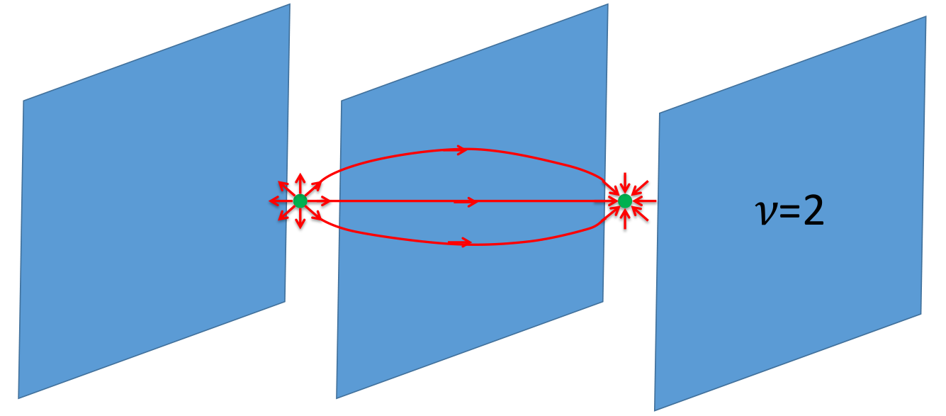
How does the symmetry in the bulk and on the surface interplay with symmetry? To answer this question, let us study the properties of the magnetic monopole in the D bulk of this phase. Imagine we have a pair of magnetic monopoles in the D bulk, each sitting between two consecutive planes and separated by a distance . When the planes are infinite, each plane between the two monopoles sees a total magnetic flux , while all other planes see magnetic flux . Now, a property of the SPT is that a flux carries a charge .33 3 Indeed, think of as two layers of IQH effect, one with and the other with . Only the electrons in the first layer are charged under . A flux induces charge in the first layer and charge in the second layer. Since only the first layer is charged under , this translates into a charge of (and charge of ). Therefore, the charge of the monopole-antimonopole configuration changes by as the distance is increased by . We conclude that and the generator of translations anti-commute on the monopole. What is the STO analogue of this effect? When a monopole tunnels across the surface of the 3+1D SPT, it leaves the anyon on the surface.44 4 Indeed, recall that the anyon created by the tunnelling event must satisfy for all anyons , where is the anyon charge. The anyons and are the only ones that satisfy this criterion. If we consider tunnelling of a neutral bulk monopole then the neutral anyon is left on the surface. As we saw in section IV, the generators of and anti-commute on , just as they do on the bulk monopole.
Appendix B Proof of existence of in a fermionic theory
Suppose we have a set of phases defined for anyons and satisfying for any with . Furthermore, assume . We claim that there exists an Abelian anyon with . Furthermore is unique up to fusion with . The proof proceeds along essentially the same lines as in the bosonic case (see section II of Ref. 20). Indeed, let . Then is a character of the fusion algebra of , i.e. it satisfies
| (78) |
Indeed, for contributing to the sum above and . Now, the algebra should admit exactly characters - the number of anyons in . By Verlinde formula, at least some of the characters can be obtained from the -matrix of : an anyon generates a character, . In fact, this generates all the characters with (of which there are ), i.e. the characters that we are interested in.
To see this, it is actually more convenient to work with an abstract theory where anyons and of are identified.[49] This theory, which we call , has half the anyons of . Fusion in is defined as , and does not depend on the representatives of equivalence classes . Fusion in is associative, commutative and each element possesses a unique inverse. We can also form a modified -matrix, , which again does not depend on the choice of representatives. In fact, is a unitary matrix.[49] Any character of with projects to a character of . Thus, are characters of . Since is unitary, this provides all distinct characters of . Therefore, we conclude that our can be written as for some , which is unique up to .
It remains to show that if is a pure phase for all then must be Abelian. As in the bosonic case,[20] this follows from unitarity of . Indeed,
| (79) | |||||
So .
References
- [1] X. Chen, Z.-C. Gu, Z.-X. Liu, and X.-G. Wen, Phys. Rev. B 87, 155114 (2013).
- [2] R. Dijkgraaf and E. Witten, Communications in Mathematical Physics 129, 393 (1990).
- [3] M. Levin and Z.-C. Gu, Phys. Rev. B 86, 115109 (2012).
- [4] X. Chen, Z.-X. Liu, and X.-G. Wen, Phys. Rev. B 84, 235141 (2011).
- [5] A. Vishwanath and T. Senthil, Phys. Rev. X 3, 011016 (2013).
- [6] M. A. Metlitski, C. L. Kane, and M. P. A. Fisher, Phys. Rev. B 92, 125111 (2015), 1306.3286.
- [7] X. Chen, L. Fidkowski, and A. Vishwanath, Phys. Rev. B 89, 165132 (2014).
- [8] P. Bonderson, C. Nayak, and X.-L. Qi, Journal of Statistical Mechanics: Theory and Experiment 2013, P09016 (2013).
- [9] C. Wang, A. C. Potter, and T. Senthil, Phys. Rev. B 88, 115137 (2013).
- [10] L. Fidkowski, X. Chen, and A. Vishwanath, Phys. Rev. X 3, 041016 (2013).
- [11] F. J. Burnell, X. Chen, L. Fidkowski, and A. Vishwanath, ArXiv e-prints (2013), 1302.7072.
- [12] X. Chen, F. J. Burnell, A. Vishwanath, and L. Fidkowski, Phys. Rev. X 5, 041013 (2015).
- [13] X. Chen, Z.-C. Gu, and X.-G. Wen, Phys. Rev. B 83, 035107 (2011).
- [14] L. Fidkowski and A. Kitaev, Phys. Rev. B 83, 075103 (2011).
- [15] F. Pollmann, A. M. Turner, E. Berg, and M. Oshikawa, Phys. Rev. B 81, 064439 (2010).
- [16] Y.-M. Lu and A. Vishwanath, Phys. Rev. B 86, 125119 (2012).
- [17] N. Bultinck, R. Vanhove, J. Haegeman, and F. Verstraete, ArXiv e-prints (2017), 1710.02314.
- [18] C.-M. Chang, Y.-H. Lin, S.-H. Shao, Y. Wang, and X. Yin, ArXiv e-prints (2018), 1802.04445.
- [19] C. Wang, C.-H. Lin, and M. Levin, Phys. Rev. X 6, 021015 (2016).
- [20] M. Barkeshli, P. Bonderson, M. Cheng, and Z. Wang, ArXiv e-prints (2014), 1410.4540.
- [21] J. C. Y. Teo, T. L. Hughes, and E. Fradkin, Annals of Physics 360, 349 (2015).
- [22] N. Tarantino, N. Lindner, and L. Fidkowski, New Journal of Physics 18, 035006 (2016).
- [23] P. Etingof, D. Nikshych, V. Ostrik, and Ehud Meir, ArXiv e-prints (2009), 0909.3140.
- [24] L. Fidkowski and A. Vishwanath, Phys. Rev. B 96, 045131 (2017).
- [25] R. Thorngren and C. von Keyserlingk, ArXiv e-prints (2015), 1511.02929.
- [26] A. Kapustin and R. Thorngren, ArXiv e-prints (2013), 1309.4721.
- [27] F. Benini, C. Cordova, and P.-S. Hsin, ArXiv e-prints (2018), 1803.09336.
- [28] M. Z. Hasan and C. L. Kane, Rev. Mod. Phys. 82, 3045 (2010).
- [29] A. Kitaev, Periodic table for topological insulators and superconductors, in American Institute of Physics Conference Series, edited by V. Lebedev and M. Feigel’Man, , American Institute of Physics Conference Series Vol. 1134, pp. 22–30, 2009, 0901.2686.
- [30] A. P. Schnyder, S. Ryu, A. Furusaki, and A. W. W. Ludwig, Phys. Rev. B 78, 195125 (2008).
- [31] A. Kapustin and R. Thorngren, Journal of High Energy Physics 2017, 80 (2017).
- [32] Q.-R. Wang and Z.-C. Gu, ArXiv e-prints (2017), 1703.10937.
- [33] M. Cheng, N. Tantivasadakarn, and C. Wang, ArXiv e-prints (2017), 1705.08911.
- [34] Z.-C. Gu and X.-G. Wen, Phys. Rev. B 90, 115141 (2014).
- [35] J. Wang et al., ArXiv e-prints (2018), 1801.05416.
- [36] X.-L. Qi, New Journal of Physics 15, 065002 (2013), 1202.3983.
- [37] S. Ryu and S.-C. Zhang, Phys. Rev. B 85, 245132 (2012).
- [38] Z.-C. Gu and M. Levin, Phys. Rev. B 89, 201113 (2014).
- [39] A. Kapustin and R. Thorngren, Phys. Rev. Lett. 112, 231602 (2014).
- [40] C. Wang and M. Levin, Phys. Rev. B 91, 165119 (2015).
- [41] X. Chen, Y.-M. Lu, and A. Vishwanath, Nature Communications 5 (2014).
- [42] C. Wang and M. Levin, Phys. Rev. Lett. 113, 080403 (2014).
- [43] Indeed, consider the topological order with the fermion parity gauged. There are 16 such modular extensions, corresponding to the 16 modular extensions of . By pasting on a suitable number of symmetric superconductors (e.g. constructed from fermions neutral under ) we can ensure that the modular extension is the toric code , with , - the fermion parity fluxes. Since the original anyons are not permuted by , consistency with fusion/braiding requires that under either or . In the second case, we can paste on an SPT. When the fermion parity in such an SPT is gauged, one gets the toric code with . So, pasting on this SPT makes and under . Then none of the anyons in the modular extension are permuted by , which means that the defect must be Abelian.
- [44] This is the first hint that the transformation has a mixed anomaly with the symmetry.
- [45] M. Cheng, M. Zaletel, M. Barkeshli, A. Vishwanath, and P. Bonderson, Phys. Rev. X 6, 041068 (2016).
- [46] J. Wang, X.-G. Wen, and E. Witten, ArXiv e-prints (2017), 1705.06728.
- [47] Indeed, think of as two layers of IQH effect, one with and the other with . Only the electrons in the first layer are charged under . A flux induces charge in the first layer and charge in the second layer. Since only the first layer is charged under , this translates into a charge of (and charge of ).
- [48] Indeed, recall that the anyon created by the tunnelling event must satisfy for all anyons , where is the anyon charge. The anyons and are the only ones that satisfy this criterion. If we consider tunnelling of a neutral bulk monopole then the neutral anyon is left on the surface.
- [49] T. Lan, L. Kong, and X.-G. Wen, Phys. Rev. B 94, 155113 (2016).