Bound on Eigenstate Thermalization from Transport

Thermalization of isolated quantum systems has attracted significant attention recently. For the quantum ergodic systems without local integrals of motion it is currently accepted that thermalization can be explained with the help of the Eigenstate Thermalization Hypothesis (ETH) [1, 2, 3, 4, 5, 6, 7, 8]. At the technical level the ETH can be understood as an ansatz for the matrix elements of observables in the energy eigenbasis [5],

Here $A$ is an observable satisfying ETH (1), $\Omega(E)dE$ is the density of states, $A^{\rm eth}$ and $f$ are smooth functions of their arguments, and $r_{ij}$ are pseudo-random fluctuations with unit variance. The diagonal part of the ETH ansatz explains thermalization, at least in the sense that the expectation value of $A$ in some initial state with mean energy $E$, after averaging over time, is equal to thermal expectation value of $A$ at the effective temperature $\beta^{-1}(E)=d\ln\Omega/dE$. The dynamics of thermalization is encoded in the off-diagonal matrix elements $r_{ij}$, as well as in the initial state $\Psi$, and is not universal. In this paper we show that macroscopic thermalization, in particular the type of transport present in the system, imposes constraints on the correlations of $r_{ij}$.

Numerical studies confirm that the $r_{ij}$ behave “randomly” and oscillate around zero mean seemingly without any obvious pattern. Certainly the $r_{ij}$ can not be random in the literal sense as the form of $A_{ij}$ is fixed once the Hamiltonian and $A$ are specified. Moreover, $A$ often has to satisfy various algebraic relations. For example, in a spin lattice model one can choose $A$ to be a Pauli matrix acting on a particular site. In this case $A^{2}={\mathbb{I}}$, which requires $r_{ij}$ to be correlated. Similarly, the $r_{ij}$ can be constrained by the expected behavior of the four-point correlation function [9, 10, 11, 12], etc.

While the whole matrix $r_{ij}$ can not be random, there is a strong expectation that fluctuations $r_{ij}$ can be treated as random if the indexes $i,j$ are restricted to belong to a sufficiently narrow energy interval. Assuming the interval is centered around some $E$, we define $\Delta E_{\rm RMT}$ as the largest possible interval such that all $r_{ij}$ with

can be treated for physical purposes as being random and independent (without necessary being normally distributed). The expectation that $r_{ij}$ reduces to a Gaussian Random Matrix inside a sufficiently narrow interval is consistent with numerical studies which confirm that the $r_{ij}$ are normally distributed [13, 14, 15] and that the form-factor $f$ becomes constant for $\omega$ smaller than inverse thermalization timescale $2\pi/\tau$, called Thouless energy¹¹ 1 Thouless energy $\Delta E_{\rm Th}$ is often defined as a scale of applicability of RMT to describe statistics of energy spectrum. Thermalization time $\tau$ is defined as time when the autocorrelation function of an operator $A$ approximately saturates to a constant. The inverse scale $2\pi/\tau$ is the size of the “plateau” of $f^{2}(\omega)$, and is also called Thouless energy in the literature. For certain systems and operators probing slowest thermalization mode both quantities are known to coincide $\Delta E_{\rm Th}\approx 2\pi/\tau$ [16, 17, 18]. [19, 17, 20, 21]. Furthermore, for real symmetric $A_{ij}$ the variances of the diagonal and off-diagonal elements have been numerically shown to satisfy $\langle r_{ii}^{2}\rangle=2\langle r_{ij}^{2}\rangle$ [22, 23, 24], which is consistent with and necessary for $r_{ij}$ to become a Gaussian Orthogonal Ensemble. Random behavior of $r_{ij}$ also naturally emerges in the recent attempt to justify ETH analytically [25]. From the physical point of view the “structureless” form of $A_{ij}$ inside a small energy interval is expected on the grounds of the hypothetical universal behavior of observables at late times [26, 27, 28, 29, 30, 31, 32, 33].

Reduction of $r_{ij}$ to an RMT below $2\pi/\tau$ is seemingly in agreement with the conventional picture of thermalization. Assuming $\tau$ is the characteristic time of the slowest transport mode probed by $A$, after the time $t\gtrsim\tau$ the system will be in the ergodic regime, i.e. value of $A$ will not be sensitive to the initial state. This suggests $r_{ij}$ should become structureless for $\Delta E_{\rm RMT}\sim 2\pi/\tau$ [17, 21]. In this Letter we show this is not the case, and $\Delta E_{\rm RMT}$ has to be parametrically smaller than the Thouless energy $2\pi/\tau$.

The key observation is that the ETH ansatz (1) with random mutually-independent $r_{ij}$ is constrained by presence of states with extensively long thermalization times. Let us consider an initial state $|\Psi\rangle$, which describes an out-of-equilibrium configuration with an order one overlap with the slowest mode probed by $A$. Then at late times

where

Here second term is simply the equilibrated value of $A$, such that $\delta A$ asymptotes to zero at late times. We also assume $|\Psi\rangle$ has less than extensive energy variance $\Delta E$. While our argument is more general, for concreteness one can think of a 1D spin chain of length $L$ exhibiting diffusive transport of energy, and $A$ would be a local operator coupled to energy. In this case the initial state can be taken to describe a quasi-classical configuration with an extensive displacement of energy, while timescale in (3) would be diffusive time $\tau\approx L^{2}/D$. An explicit construction of such a state $|\Psi\rangle$ is given in the Supplemental Materials (SM).

To connect thermalization time $\tau$ to matrix elements of $A$ we introduce a parameter-dependent average, which is somewhat similar to the “average distance” used in [34],

Here $T$ is a free parameter. When $T$ becomes large, (5) reduced to the conventional average over time $T$. After representing $A(t)$ in the energy eigenbasis using (1) and performing the integral in (5) we find

where the operator $\delta A_{T}$ written in the energy eigenbasis has the form

In other words the matrix $(\delta A_{T})_{ij}$ has a band structure, it coincides with $A_{ij}$ (after subtracting the non-random diagonal part) inside a diagonal band of size $2\pi/T$, and is zero outside. This is schematically shown in Fig. 1.

The expectation value $\langle\Psi|\delta A_{T}|\Psi\rangle$ can be bounded by the largest eigenvalue of $\delta A_{T}$, which we denote by $x(T)$,

Let us assume now that $T$ is sufficiently large such that $2\pi/T\leq\Delta E_{RMT}$. Then $(\delta A_{T})_{ij}$ is a band random matrix with independent matrix elements and its largest eigenvalue is controlled by the variance function $\overline{(\delta A_{T})^{2}_{ij}}=\Omega^{-1}f^{2}(\omega)$ [35]. In the limit of a narrow band $T\Delta E\gg 1$, see SM,

Technically, (11) assumes absence of correlations, while the definition of $\Delta E_{RMT}$ (2) does not exclude possible correlations of $r_{ij}$ and $r_{i^{\prime}j^{\prime}}$ along the diagonal, i.e. when $(E_{i}+E_{j})-(E_{i}^{\prime}+E_{j}^{\prime})$ is large while $|E_{i}-E_{j}|$ and $|E_{i^{\prime}}-E_{j^{\prime}}|$ are small. In SM we justify (11) rigorously, using the result of [22], by converting it into an inequality. Looking ahead, our main result, inequality (13), continue to hold with different numerical coefficients.

With help of (1) the integral in the right-hand-side of (11) can be expressed through the connected autocorrelation function of $A$ calculated at the effective inverse temperature $\beta^{-1}=d\ln\Omega/dE$ [19, 20, 17],

Now combining (10) with (11) written with help of (12) we find the inequality, which should be satisfied so far $T\geq T_{\rm RMT}\equiv 2\pi/\Delta E_{\rm RMT}$,

The inequality (13) is our main technical result, which implies strong limitations on $\Delta E_{\rm RMT}$. As the characteristic size $L$ of the system grows, the autocorrelation function of $A$ approaches its thermodynamic form, which follows from quasi-classical hydrodynamic description,

with some $L$-independent $\alpha>0$ and $t_{D}$. Coefficient $\alpha$ depends on the type of transport $A$ couples to. The behavior (14) applies for $t\gtrsim t_{D}$ and persists until $t\approx\tau$, after which the autocorrelation function becomes zero [17, 20]. Around the time $t\approx\tau$ the value of full autocorrelation function, i.e. without the asymptotic value subtracted, should be inverse proportional to volume, indicating that the conserved quantity coupled to $A$ has spread across the whole system

Here $L$ is a characteristic size of the system in dimensional units, e.g. the number of spins, while $d$ is the number of spatial dimensions. Using (14), and for $T\gg t_{D}$ the right-hand-side of (13) can be approximated as follows, where we dropped all numerical coefficients,

For late times $T\gg t_{D}$ (16) is very small irrespective of the value of $\tau/T$. Strictly speaking the estimate above is only correct far $\alpha<1$ such that the integral gets its main contribution for large $t$. In most cases this requires $d=1$.

The behavior of the left-hand-side of (13) is quite different. Starting from the expoential decay (3) we find for large $T\gg\tau$,

which is in agreement with the qualitative picture that $\delta A(t,\Psi)$ remains of order one for the time $t\sim\tau$ and then quickly approaches zero. When $T$ is large but not necessarily larger than $\tau$ (20) remains of order one and the inequality (13) can not be satisfied. For (13) to be satisfied $T$ has to be parametrically larger than $\tau$,

To summarize, we see that the inequality (13) imposes a stringent bound on the energy scale $\Delta E_{\rm RMT}=2\pi/T_{\rm RMT}$, which should be parametrically smaller than the Thouless energy $2\pi/\tau$. In particular, for a 1D diffusive system and a local operator $A$ coupled to conserved quantity we find

More generally, for any 1D system with local interactions transport can not be faster than ballistic, $\tau\propto L$, and therefore for any local operator, $T_{\rm RMT}\gtrsim\tau L\sim L^{2}$.

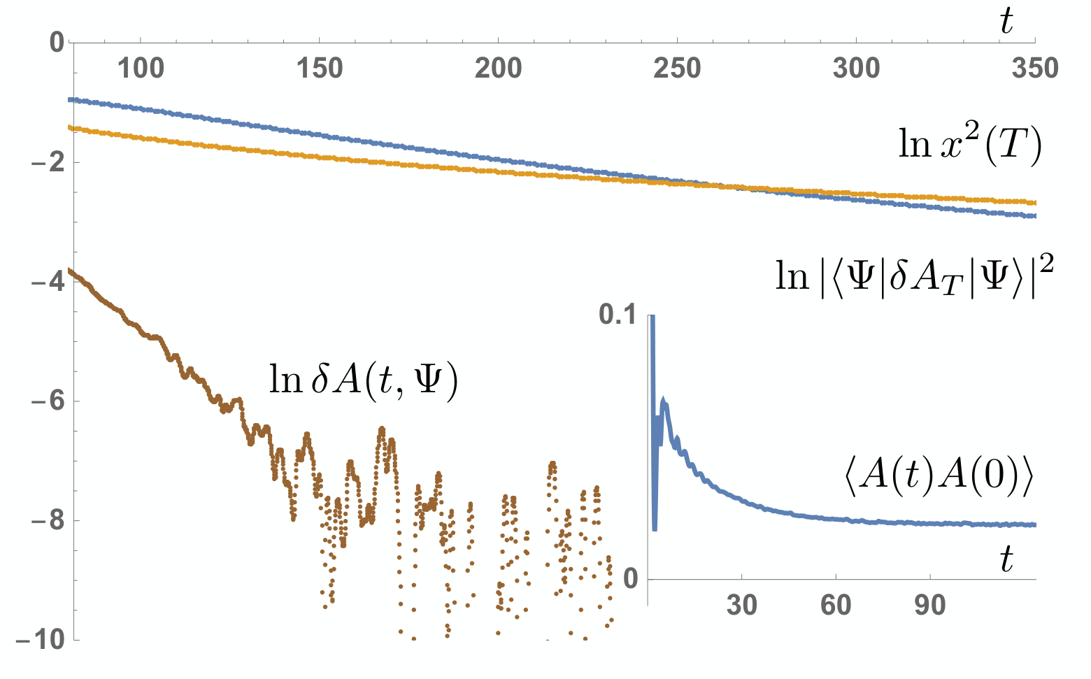
We illustrate the inequality (13) and the resulting difference between $\Delta E_{\rm RMT}$ and $\tau^{-1}$ with help of an open non-integrable 1D Ising spin-chain with two polarizations of magnetic field. The operator $A=\sigma_{x}^{1}$ is a one-site operator. This model is diffusive. In SM, where all technical details can be found, we numerically justify (3) as well as (14) with $\alpha=1/2$. The result, the left-hand-side and the right-hand-side of (13), is shown in Fig. 2. The inequality is saturated for times $T$ significantly larger than thermalization time $\tau$, when the autocorrelation function plateaus (see the inset). This confirms the conclusion that the RMT time scale $T_{\rm RMT}$ is much larger than thermalization time. Smallness of $\tau/T_{\rm RMT}\ll 1$ was also recently confirmed numerically in [24, 36].

For a translationally-invariant system it is also interesting to consider an operator $A_{k}$ with a constant momentum. Keeping in mind a 1D diffusive spin lattice system of length $L$, we denote by $A_{(m)}$ a local operator $A$ located at the site $m$. Then

where $L$ is dimensionless. The normalization factor $(2/L)^{1/2}$ is chosen such that the connected autocorrelation function is $L$-independent in the thermodynamic limit

With the same normalization the expectation value (4) in the state with a macroscopic amount of energy displaced will be

Although the $t$-dependence in (24) and (25) is the same, different $L$-dependent prefactor will result in a constraint for $T_{\rm RMT}$. For large $T\gg\tau_{k}$ we can estimate

After ignoring unimportant numerical prefactors (13) yields, in agreement with (21),

To conclude, we have shown that the energy scale $\Delta E_{\rm RMT}$ at which the ETH ansatz reduces to Random Matrix Theory has to be parametrically smaller than the inverse thermalization time, i.e. characteristic time of the slowest mode probed by the corresponding operator. For a 1D system and a local operator $A$ coupled to diffusive quantity we found $\Delta E_{\rm RMT}$ to be bounded by $(\tau L)^{-1}\sim L^{-3}$, where $L$ is the system size and $\tau\approx L^{2}/D$ is the diffusion time.

Our result (13,21) is an inequality, which raises the question of identifying the correct scaling of $\Delta E_{\rm RMT}$ with the system size and understanding significance of the associated timescale $T_{\rm RMT}=2\pi/\Delta E_{\rm RMT}^{-1}$ from the point of view of thermalization dynamics. We conjecture (21) reflects the correct scaling $T_{\rm RMT}\propto\tau L^{d}$ and propose the following interpretation. The timescale $T_{\rm RMT}$ which marks the onset of random matrix behavior for an observable $A$ coincides with the end of macroscopic thermalization, i.e. applicability of hydrodynamic description of transport. The expectation value $\delta A(t,\Psi)\sim e^{-t/\tau}$ will decay exponentially until it saturates into exponentially small fluctuations of order $e^{-S/2}$, where $S\propto L^{d}$ is entropy. This happens around time

which we conjecture to agree with $T_{\rm RMT}$ up to constant prefactors. This interpretation, and scaling, is consistent with the onset of RMT-defined universal behavior of autocorrelation function at late times [37, 38]. It is also consistent with the numerics shown in Fig. 2, where by the time the inequality (13) is satisfied the expectation value $\delta A(t,\Psi)$ has firmly saturated into the asymptotic fluctuation regime.

References

- [1] R. Jensen and R. Shankar, Physical review letters 54, 1879 (1985).
- [2] J. M. Deutsch, Physical Review A 43, 2046 (1991).
- [3] M. Srednicki, Physical Review E 50, 888 (1994).
- [4] M. Srednicki, Journal of Physics A: Mathematical and General 29, L75 (1996).
- [5] M. Srednicki, Journal of Physics A: Mathematical and General 32, 1163 (1999).
- [6] M. Rigol, V. Dunjko, and M. Olshanii, Nature 452, 854 (2008).
- [7] M. Rigol and M. Srednicki, Physical review letters 108, 110601 (2012).
- [8] G. De Palma, A. Serafini, V. Giovannetti, and M. Cramer, Physical review letters 115, 220401 (2015).
- [9] L. Foini and J. Kurchan, Phys. Rev. E 99, 042139 (2019a).
- [10] A. Chan, A. De Luca, and J. T. Chalker, Phys. Rev. Lett. 122, 220601 (2019).
- [11] L. Foini and J. Kurchan, Phys. Rev. Lett. 123, 260601 (2019b).
- [12] M. Brenes, S. Pappalardi, M. T. Mitchison, J. Goold, and A. Silva, Phys. Rev. E 104, 034120 (2021).
- [13] W. Beugeling, R. Moessner, and M. Haque, Physical Review E 89, 042112 (2014).
- [14] W. Beugeling, R. Moessner, and M. Haque, Physical Review E 91, 012144 (2015).
- [15] A. Dymarsky, N. Lashkari, and H. Liu, Physical Review E 97, 012140 (2018).
- [16] A. Altland, Y. Gefen, and G. Montambaux, Phys. Rev. Lett. 76, 1130 (1996).
- [17] L. D’Alessio, Y. Kafri, A. Polkovnikov, and M. Rigol, Advances in Physics 65, 239 (2016).
- [18] M. Sonner, M. Serbyn, Z. Papić, and D. A. Abanin, Phys. Rev. B 104, L081112 (2021).
- [19] E. Khatami, G. Pupillo, M. Srednicki, and M. Rigol, Physical review letters 111, 050403 (2013).
- [20] D. J. Luitz and Y. B. Lev, Physical review letters 117, 170404 (2016).
- [21] M. Serbyn, Z. Papić, and D. A. Abanin, Physical Review B 96, 104201 (2017).
- [22] A. Dymarsky and H. Liu, Phys. Rev. E 99, 010102 (2019).
- [23] R. Mondaini and M. Rigol, Physical Review E 96, 012157 (2017).
- [24] J. Richter, A. Dymarsky, R. Steinigeweg, and J. Gemmer, Phys. Rev. E 102, 042127 (2020), arXiv:2007.15070 [cond-mat.stat-mech] .
- [25] F. Anza, C. Gogolin, and M. Huber, Physical Review Letters 120, 150603 (2018).
- [26] J. S. Cotler, G. Gur-Ari, M. Hanada, J. Polchinski, P. Saad, S. H. Shenker, D. Stanford, A. Streicher, and M. Tezuka, Journal of High Energy Physics 2017, 118 (2017a).
- [27] J. Cotler, N. Hunter-Jones, J. Liu, and B. Yoshida, Journal of High Energy Physics 2017, 48 (2017b).
- [28] L. F. Santos and E. Torres-Herrera, arXiv preprint arXiv:1803.06012 (2018).
- [29] S. Moudgalya, T. Devakul, C. W. von Keyserlingk, and S. L. Sondhi, Phys. Rev. B 99, 094312 (2019).
- [30] M. Schiulaz, E. J. Torres-Herrera, and L. F. Santos, Phys. Rev. B 99, 174313 (2019).
- [31] A. Belin, J. de Boer, and D. Liska, (2021a), arXiv:2110.14649 [hep-th] .
- [32] A. Belin, J. de Boer, P. Nayak, and J. Sonner, (2021b), arXiv:2111.06373 [hep-th] .
- [33] C.-F. Chen and F. G. S. L. Brandão, (2021), arXiv:2112.07646 [quant-ph] .
- [34] L. P. García-Pintos, N. Linden, A. S. Malabarba, A. J. Short, and A. Winter, Physical Review X 7, 031027 (2017).
- [35] S. A. Molchanov, L. A. Pastur, and A. Khorunzhii, Theoretical and Mathematical Physics 90, 108 (1992).
- [36] J. Wang, M. H. Lamann, J. Richter, R. Steinigeweg, A. Dymarsky, and J. Gemmer, (2021), arXiv:2110.04085 [cond-mat.stat-mech] .
- [37] L. V. Delacretaz, SciPost Phys. 9, 34 (2020).
- [38] T. L. M. Lezama, E. J. Torres-Herrera, F. Pérez-Bernal, Y. Bar Lev, and L. F. Santos, Phys. Rev. B 104, 085117 (2021).
- [39] E. H. Lieb and D. W. Robinson, in Statistical Mechanics (Springer, 1972) pp. 425–431.
- [40] M. B. Hastings, Quantum Theory from Small to Large Scales 95, 171 (2010).
- [41] V. K. Varma, A. Lerose, F. Pietracaprina, J. Goold, and A. Scardicchio, Journal of Statistical Mechanics: Theory and Experiment 2017, 053101 (2017).
- [42] T. A. Elsayed and B. V. Fine, Phys. Rev. Lett. 110, 070404 (2013).
- [43] A. Stathopoulos and J. R. McCombs, ACM Transactions on Mathematical Software (TOMS) 37, 1 (2010).