Solutions of a two-particle interacting quantum walk
Abstract
We study the solutions of the interacting Fermionic cellular automaton introduced in Ref. Bisio et al. (2018). The automaton is the analogue of the Thirring model with both space and time discrete. We present a derivation of the two-particles solutions of the automaton, which exploits the symmetries of the evolution operator. In the two-particles sector, the evolution operator is given by the sequence of two steps, the first one corresponding to a unitary interaction activated by two-particle excitation at the same site, and the second one to two independent one-dimensional Dirac quantum walks. The interaction step can be regarded as the discrete-time version of the interacting term of some Hamiltonian integrable system, such as the Hubbard or the Thirring model. The present automaton exhibits scattering solutions with nontrivial momentum transfer, jumping between different regions of the Brillouin zone that can be interpreted as Fermion-doubled particles, in stark contrast with the customary momentum-exchange of the one dimensional Hamiltonian systems. A further difference compared to the Hamiltonian model is that there exist bound states for every value of the total momentum, and even for vanishing coupling constant. As a complement to the analytical derivations we show numerical simulations of the interacting evolution.
keywords
Quantum walks; Hubbard model; Thirring modelPACS
71.10.Fd, 03.67.Ac10.3390/—— \historyReceived: date; Accepted: date; Published: date \orcidauthorONE0000-0000-000-000X
1 Introduction
Quantum walks (QWs) describe the evolution of one-particle quantum states on a lattice, or more generally, on a graph. The quantum walk evolution is linear in the quantum state and the quantum aspect of the evolution occurs in the interference between the different paths available to the walker. There are two kinds of quantum walks: continuous time QWs, where the evolution operator of the system given in terms of an Hamiltonian can be applied at any time (see Farhi et al. Farhi et al. (2008)), and discrete-time QWs, where the evolution operator is applied in discrete unitary time-steps. The discrete-time model, which appeared already in the Feynman discretization of the Dirac equation Feynman et al. (1965), was later rediscovered in quantum information Grossing and Zeilinger (1988); Ambainis et al. (2001); Reitzner et al. (2011); Gross et al. (2012); Shikano (2013), and proved to be a versatile platform for various scopes. For example, QWs have been used for empowering quantum algorithms, such as database search Childs and Goldstone (2004); Portugal (2013), or graph isomorphism Douglas and Wang (2008); Gamble et al. (2010). Moreover, quantum walks have been studied as a simulation tool for relativistic quantum fields Bialynicki-Birula (1994); Meyer (1996); Yepez (2006); Arrighi and Facchini (2013); Bisio et al. (2015); D’Ariano and Perinotti (2014); D’Ariano et al. (2014); D’Ariano et al. (2015); Arrighi et al. (2016); Bisio et al. (2016); Arnault and Debbasch (2016); Bisio et al. (2016); Mallick et al. (2017); Molfetta and Pérez (2016); Brun and Mlodinow (2018a); Brun and Mlodinow (2018b), and they have been used as discrete models of spacetime Bibeau-Delisle et al. (2015); Bisio et al. (2016a); Bisio et al. (2016b); Arrighi et al. (2014).
QWs are among the most promising quantum simulators with possible realizations in a variety of physical systems, such as nuclear magnetic resonance Du et al. (2003); Ryan et al. (2005), trapped ions Xue et al. (2009), integrated photonics, and bulk optics Do et al. (2005); Sansoni et al. (2012); Crespi et al. (2013); Flamini et al. (2018).
New research perspectives are unfolding in the scenario of multi-particle interacting quantum walks where two or more walking particles are coupled via non-linear (in the field) unitary operators. The properties of these systems are still largely unexplored. Both continuous-time Childs (2009) and discrete-time Lovett et al. (2010) quantum walks on sparse unweighted graphs are equivalent in power to the quantum circuit model. However, it is highly non trivial to design a suitable architecture for universal quantum computation based on quantum walks. Within this perspective a possible route has been suggested in Ref. Childs et al. (2013) based on interacting multi-particle quantum walks with indistinguishable particles (Bosons or Fermions), proving that “almost any interaction” is universal. Among the universal interacting many-body systems are the models with coupling term of the form , with the number operator at site . The latter two-body interaction lies at the basis of notable integrable quantum systems in one space dimension such as the Hubbard and the Thirring Hamiltonian models.
The first attempt at the analysis of interacting quantum walks was carried out in Ref. Ahlbrecht et al. (2012). More recently, in Ref. Bisio et al. (2018), the authors proposed a discrete-time analogue of the Thirring model which is indeed a Fermionic quantum cellular automaton, whose dynamics in the two-particles sector reduces to an interacting two-particle quantum walk. As for its Hamiltonian counterpart, the discrete-time interacting walk has been solved analytically in the case of two Fermions. Analogously to any Hamiltonian integrable system, also in the discrete-time case the solution is based on the Bethe Ansatz technique. However, discreteness of the evolution prevents the application of the usual Ansatz, and a new Ansatz has been introduced successfully Bisio et al. (2018).
In this paper we present an original simplified derivation of the solution of Ref. Bisio et al. (2018) which exploits the symmetries of the interacting walk. We present the diagonalization of the evolution operator and the characterization of its spectrum. We explicitly write the two particle states corresponding to the scattering solutions of the system, having eigenvalues in the continuous spectrum of the evolution operator. We then show how the present model predicts the formation of bound states, which are eigenstates of the interacting walk corresponding to the discrete spectrum. We provide also in this case the analytic expression of such molecular states.
We remark the phenomenological differences between the Hamiltonian model and the discrete-time one. First we see that the set of possible scattering solutions is larger in the discrete-time case: for a fixed value total momentum, a non trivial transfer of relative momentum can occur besides the simple exchange of momentum between the two particles, differently from the Hamiltonian case. Also the family of bound states appearing in the discrete-time scenario is larger than the corresponding Hamiltonian one. Indeed, for any fixed value of the coupling constant, a bound state exists with any possible value of the total momentum, while for Hamiltonian systems bound states cannot have arbitrary total momentum.
Finally we show that in the set of solutions for the interacting walk there are perfectly localized states (namely states which lie on a finite number of lattice sites) and, differently from the Hamiltonian systems, bound states exist also for vanishing coupling constant. In addition to the exact analytical solution of the dynamics we show the simulation of some significant initial state.
2 The Dirac Quantum Walk
In this section, we review the Dirac walk on the line describing the free evolution of a two-component Fermionic field. The walk evolution is provided by the unitary operator acting on the single particle Hilbert space for which we employ the factorized basis , with and . Being the evolution of a quantum walk linear in the field operators, the single-step evolution is expressed by the following equation:
with given by
| (1) |
where denotes the translation operator on , defined by .
Since the walk is translation invariant (it commutes with the translation operator), it can be diagonalized in momentum space. In the momentum representation, defining , with , the walk operator can be written as
where . The spectrum of the walk is given by , where the dispersion relation is given by
| (2) |
where denotes the principal value of the arccosine function. The single-particle eigenstates, solving the eigenvalue problem
| (3) |
can be conveniently written as
with , .
3 The Thirring Quantum Walk
In this section we present a Fermionic cellular automaton in one spatial dimension with an on-site interaction, namely two particles interact only when they lie at the same lattice site. The linear part corresponds to the Dirac QW D’Ariano and Perinotti (2014) and the interaction term is the most general number-preserving coupling in one dimension Östlund and Mele (1991). The same kind of interaction characterizes also the most studied integrable quantum systems, such as the Thirring Thirring (1958) and the Hubbard Hubbard (1963) models.
The linear part of the -particle walk is described by the operator , acting on the Hilbert space and describing the free evolution of the particles. In order to introduce an interaction, we modify the update rule of the walk with an extra step : . In the present case the term has the form
where , , represents the particle number at site , namely , and is a real coupling constant. Since the interaction term preserves the total number operator we can study the walk dynamics for a fixed number of particles. In this work we focus on the two-particle sector whose solutions has been derived in Ref. Bisio et al. (2018). As we will see, the Thirring walk features molecule states besides scattering solutions. This features is shared also by the Hadamard walk with the same on-site interaction Ahlbrecht et al. (2011).
Since we focus on the solutions involving the interaction of two particles, it is convenient to write the walk in the centre of mass basis , with , and . Therefore in this basis the generic Fermionic state is with . Notice that only the pairs with and both even or odd correspond to physical points in the original basis .
We define the two-particle walk with both and in , so that the linear part of walk can be written as
| (4) |
where represents the translation operator in the relative coordinate , and the translation operator in the centre of mass coordinate , whereas the interacting term reads
This definition gives a walk that can be decomposed in two identical copies of the original walk. Indeed, defining as the projector on the physical center of mass coordinates, one has , where and are unitarily equivalent. We will then diagonalize the operator , reminding that the physical solutions will be given by projecting the eigenvectors with .
Introducing the (half) relative momentum and the (half) total momentum , the free evolution of the two particles is written in the momentum representation as
| where the matrix is defined as | ||||
| Furthermore, we introduce the vectors , with , such that | ||||
where is the dispersion relation of the two-particle walk. Explicitly, the vectors are given by
| (5) |
We focus in this work on Fermionic solutions satisfying the eigenvalue equation
| (6) |
with . In the centre of mass basis the antisymmetry condition reads
| being the exchange matrix | |||
4 Symmetries of the Thirring Quantum Walk
The Thirring walk manifests some symmetries that allow to simplify the derivation and the study of the solutions. First of all, as we already mentioned, one can show that the interaction commutes with the total number operator. This means that one can study the walk dynamics separately for each fixed number of particles. We focus here on the two-particle walk , where and .
Since the interacting walk commutes with the translations in the centre of mass coordinate , the total momentum is a conserved quantity, so it is convenient to study the walk parameterized by the total momentum . To this end we consider the basis , so that for fixed values of the interacting walk of two particles can be expressed in terms of a one-dimensional QW with a four dimensional coin:
Although the range of the variable is the interval , it is possible to show that one can restrict the study of the walk to the interval . On the one hand, the two-particle walk transforms unitarily under a parity transformation in the momentum space. Starting from the single particle walk, transforms under a parity transformation as
so that for the two-particle walk we have the relation
On the other hand, a translation of of the total momentum entails that
| (7) |
while the interaction term remains unaffected in both cases.
The Thirring walk features also another symmetry that can be exploited to simplify the derivation of the solutions. It is easy to check that the walk operator commutes with the projector defined by
| (8) |
where and are the projectors on the even and the odd subspaces, respectively:
The projector induces a splitting of the total Hilbert space in two subspaces and , with the interaction term acting non trivially only in the subspace . In the complementary subspace the evolution is free for Fermionic particles. This means that solutions of the free theory are also solutions of the interacting one, as opposed to the Bosonic case for which the interaction is non-trivial also in .
5 Review of the solutions
We focus in this section on the antisymmetric solutions of the Thirring walk which actually feel the interaction. From the remarks that we have made in the previous section, such solutions can only be found in the subspace . Formally, we have to solve the eigenvalue equation , with . Conveniently, we write a vector in the form
| (9) |
and the antisymmetry condition becomes:
The restriction of the walk to the subspace entails that the eigenvalue problem is equivalent to the following system of equations:
| (10) |
The most general solution of eq. 10 for has two forms:
| (11) | |||
| and | |||
| (12) | |||
| with , , and satisfying the condition | |||
Solving eq. 10 corresponds now to find the function . Let us now study the equation
Since has to be an eigenvalue of , must be real and thus or with , so we conveniently define the sets:
It is easy to see that for all , and , and the range of the function covers the entire unit circle except for the points . Therefore, we can discuss separately the case and the case . A solution with actually exists, corresponding to the function of eq. 11, and it will be discussed in section 5.3.
Let us start with the case which will lead to the characterization of the continuous spectrum of the Thirring walk and of the scattering solutions.
5.1 Scattering solutions
In this section we assume with . This implies that : indeed, as one can notice from fig. 1, the lines lie entirely in the gaps between the curves and . The solution is thus the one given in eq. 12. One can prove that and . Furthermore, as one can notice from fig. 2, there are four values of the triple such that for a given value of : if the triple is a solution, so are , and ; and if is a solution, then also , and are solutions. This result greatly simplifies eq. 12. Indeed the sum over and the integral over reduces to the sum of four terms:
| (13) | ||||||
As we will see, the original problem can be simplified in this way to an algebraic problem with a finite set of equations. We remark that the fact that the equation has a finite number of solutions is a consequence of the fact that we are considering a model in one spatial dimension. However, in analogous one-dimensional Hamiltonian models (e.g. the Hubbard model) the degeneracy of the eigenvalues is two.
Let us consider for the sake of simplicity the solution of the kind , since the other one can be analysed in a similar way. Using the notation of appendix A, eq. 13 reduces to the expressions (dropping the superscript)
| (14) | ||||
We notice that now the number of unknown parameters is further reduced to three, namely , , and . Clearly, one of the parameters can be fixed by choosing arbitrarily the normalization. From now on we fix and define . eq. 14 has to satisfy the recurrence relations of eq. 10 for and , while for it is automatically satisfied. For , eq. 10 becomes
| (15) | |||||
| (16) | |||||
| (17) | |||||
| (18) |
Starting from Eq. (15), we can notice that , where we employed the notation of appendix A, so that we obtain . We can then substitute this expression in Eq. (17) and use the relations
| to obtain the expression | |||
and thus
| (19) |
For these values of and one can verify that eq. 10 is satisfied also for , thus concluding the derivation. For the solution of the kind we can follow a similar reasoning, obtaining the analogous quantity :
| (20) |
It is worth noticing that is of unit modulus for .


The final form of the solution results to be
| (21) | ||||
which in terms of the relative coordinate can be written as
We can interpret such a solution as a scattering of plane waves for which the coefficient plays the role of the transmission coefficient. Being the total momentum a conserved quantity, the two particles can only exchange their momenta, as expected from a theory in one-dimension. Furthermore, for each value of the relative momentum, the two particles can also acquire an additional phase of . As the interaction is a compact perturbation of the free evolution, the continuous spectrum is the same as that of the free walk. eq. 21 provides the generalized eigenvector if corresponding to the continuous spectrum .
5.2 Bound states
In the previous section, we derived the solutions in the continuous spectrum, which can be interpreted as scattering plane waves in one spatial dimension. We seek now the solutions corresponding to the discrete spectrum, namely solutions with eigenvalue in any one of the sets . The derivation of the solution follows similar steps as for the scattering solutions. In particular, the degeneracy in is the same: there are four solutions to the equation even in this case, as proved in Ref. Bisio et al. (2018). Therefore the general form of the solution in this case can be written again as in eq. 13 and, following the same reasoning, one obtains the same set of solutions as in eq. 21. At this stage we did not imposed that the solution is a proper eigenvector in the Hilbert space . To this end, we have to set to eliminate the exponentially-divergent terms in eq. 21. As one can prove, the equation has only one solution for fixed values of and . More precisely, there is a unique , with and , such that either or .
In other words, for each pair of values the walk has one and only eigenvector corresponding to an eigenvalue in the point spectrum. Such eigenvector can be written as
| (22) | ||||
where is the solution of or and chosen accordingly. More compactly, in the coordinate, the solution can be written as
Referring to fig. 3, we show the evolution of two particles initially prepared in a singlet state localized at the origin. From the figure one can appreciate the appearance of the bound state component which has non-vanishing overlapping with the initial state. The bound state, being exponentially decaying in the relative coordinate , is localized on the diagonal of the plot, that is when the two particles lie at the same point.
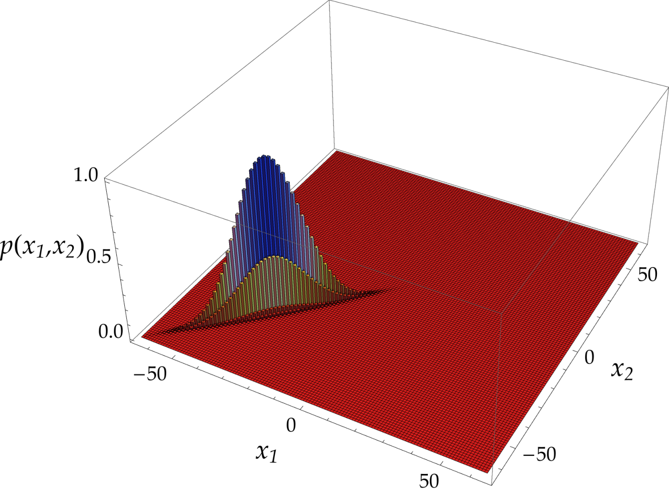
In fig. 5 is depicted the probability distribution of the bound state corresponding to choice of the parameters and . The plot highlights the exponential decay of the tails, which is the characterizing feature of the bound state.

5.3 Solution for
So far we have studied proper eigenvectors which decay exponentially as the two particles are further apart. However, the previous analysis failed to cover the particular case when , since the range of does not include the two points of the unit circle .
We study now the solutions with having the form given in eq. 11. One can prove that such solutions are non-vanishing only for on , namely we look for a solution of the form
| (23) |
Subtracting the first and the last equations of (10) using (23), we obtain the following equation:
| (24) |
If both and are non-zero, one can prove that a solution does not exist and thus we have to consider the two cases and separately. Starting from , eq. 24 imposes that , meaning that if a solution exists in this case, it is an eigenvector corresponding to the eigenvalue . From the second equation of (10) we obtain the relation
and, using the first equation of (10), it turns out that a solution exists only if , as expected since otherwise we would have been in the case of section 5.2 would hold. The other case, namely , can be studied analogously. Let us, then, denote as such proper eigenvectors with eigenvalue for and, choosing as the value for the free parameter , we obtain the following expression for :
Such solutions provide a special case of molecule states (namely, proper eigenvectors of ), being localized on few sites, and differ from the previous solutions showing an exponential decay in the relative coordinate.
5.4 Solutions for
The solutions that we presented in the previous discussion do not cover the extreme values (see Ref. Bisio et al. (2018) for a reference). Let us consider for definiteness the case since the other case is obtained in a similar way. For the previous analysis still holds. Indeed, noticing that , we have and if and only if , whereas for all . This means that the solutions of eq. 21 are actually eigenvectors of . Thus, the spectrum is made by a continuous part, given by the arc of the unit circle containing and having as extremes, and a point spectrum with two points: , where is the solution of for , and . As shown in Ref. Bisio et al. (2018), is a separated part of the spectrum of and the corresponding eigenspace is a separable Hilbert space of stationary bound states. This fact underlines an important feature of the Thirring walk not shared by analogous Hamiltonian models. It is remarkable that this behaviour occurs also for the free walk with . In fig. 6 we show the probability distribution of two states having he properties hereby discussed. It is worth noticing that all the states with are eigenvectors relative to the eigenvalue , and thus they generate a subspace on which the walk acts identically. We remark that this behaviour relies on the fact that the dispersion relation in one dimension is an even function of .
In fig. 4 is depicted the discrete spectrum of the interacting walk together with the continuous spectrum as a function of the total momentum . The solid curves in the gaps between the continuous bands denote the discrete spectrum for different values of the coupling constant . Molecule states appear also in the Hadamard walk with the same on-site interaction Ahlbrecht et al. (2011).
6 Conclusions
In this work we reviewed the Thirring quantum walk providing a simplified derivation of its solutions for Fermionic particles. The simplified derivation relies on the symmetric properties of the walk evolution operator allowing to separate the subspace of solutions affected by the interaction from the subspace where the interaction step acts trivially. The interaction term is the most general number-preserving interaction in one dimension, whereas the free evolution is provided by the Dirac QW D’Ariano and Perinotti (2014).
We showed the explicit derivation of the scattering solutions (solutions for the continuous spectrum) as well as for the bound-state solutions. The Thirring walk features also localized bound states (namely, states whose support is finite on the lattice) when . Such solutions exist only when the coupling constant is . In fig. 3 is depicted the evolution of a perfectly localized state showing the overlapping with bound states components. In fig. 5 we reported the evolution of a bound state of the two particles peaked around a certain value of the total momentum: one can appreciate that the probability distribution remains localized on the main diagonal during the evolution.
Finally, we discussed also the class of proper eigenvectors arising in the free theory highlighting another difference between the discrete model of the present work with analogous Hamiltonian models.
multiple
Appendix A Notation
For the single particle walk of eq. 1 the eigenstates can be written as
with . For the two-particle walk we define . If than we name the related eigenspace the even eigenspace; whereas, if we call the related eigenspace the odd eigenspace. As proven in item of Lemma of Ref. Bisio et al. (2018), for a given the degeneracy is both in the even and in the odd case. Namely, if the triple is a solution then also , and are solutions; if the triple is a solution, then also and are solutions.
Explicitly, for the even case we have:
Analogously for the odd case the eigenstates are
In order to simplify the derivation of the solution, we adopt the following notation:
References
- Bisio et al. (2018) Bisio, A.; D’Ariano, G.M.; Perinotti, P.; Tosini, A. Thirring quantum cellular automaton. Phys. Rev. A 2018, 97, 032132.
- Farhi et al. (2008) Farhi, E.; Goldstone, J.; Gutmann, S. A Quantum Algorithm for the Hamiltonian NAND Tree. Theory of Computing 2008, 4, 169–190.
- Feynman et al. (1965) Feynman, R.P.; Hibbs, A.R.; Styer, D.F. Quantum mechanics and path integrals; Vol. 2, International series in pure and applied physics, McGraw-Hill New York, 1965.
- Grossing and Zeilinger (1988) Grossing, G.; Zeilinger, A. Quantum cellular automata. Complex Systems 1988, 2, 197–208.
- Ambainis et al. (2001) Ambainis, A.; Bach, E.; Nayak, A.; Vishwanath, A.; Watrous, J. One-dimensional Quantum Walks. Proceedings of the Thirty-third Annual ACM Symposium on Theory of Computing; ACM: New York, NY, USA, 2001; STOC ’01, pp. 37–49.
- Reitzner et al. (2011) Reitzner, D.; Nagaj, D.; Buek, V. Quantum Walks. Acta Physica Slovaca. Reviews and Tutorials 2011, 61, 603–725.
- Gross et al. (2012) Gross, D.; Nesme, V.; Vogts, H.; Werner, R. Index theory of one dimensional quantum walks and cellular automata. Communications in Mathematical Physics 2012, pp. 1–36.
- Shikano (2013) Shikano, Y. From Discrete Time Quantum Walk to Continuous Time Quantum Walk in Limit Distribution. Journal of Computational and Theoretical Nanoscience 2013, 10, 1558–1570.
- Childs and Goldstone (2004) Childs, A.M.; Goldstone, J. Spatial search by quantum walk. Phys. Rev. A 2004, 70, 022314.
- Portugal (2013) Portugal, R. Quantum walks and search algorithms; Springer Science & Business Media, 2013.
- Douglas and Wang (2008) Douglas, B.L.; Wang, J.B. A classical approach to the graph isomorphism problem using quantum walks. Journal of Physics A: Mathematical and Theoretical 2008, 41, 075303.
- Gamble et al. (2010) Gamble, J.K.; Friesen, M.; Zhou, D.; Joynt, R.; Coppersmith, S.N. Two-particle quantum walks applied to the graph isomorphism problem. Phys. Rev. A 2010, 81, 052313.
- Bialynicki-Birula (1994) Bialynicki-Birula, I. Weyl, Dirac, and Maxwell equations on a lattice as unitary cellular automata. Physical Review D 1994, 49, 6920.
- Meyer (1996) Meyer, D. From quantum cellular automata to quantum lattice gases. Journal of Statistical Physics 1996, 85, 551–574.
- Yepez (2006) Yepez, J. Relativistic Path Integral as a Lattice-based Quantum Algorithm. Quantum Information Processing 2006, 4, 471–509.
- Arrighi and Facchini (2013) Arrighi, P.; Facchini, S. Decoupled quantum walks, models of the Klein-Gordon and wave equations. EPL (Europhysics Letters) 2013, 104, 60004.
- Bisio et al. (2015) Bisio, A.; D’Ariano, G.M.; Tosini, A. Quantum field as a quantum cellular automaton: The Dirac free evolution in one dimension. Annals of Physics 2015, 354, 244 – 264.
- D’Ariano and Perinotti (2014) D’Ariano, G.M.; Perinotti, P. Derivation of the Dirac equation from principles of information processing. Phys. Rev. A 2014, 90, 062106.
- D’Ariano et al. (2014) D’Ariano, G.M.; Mosco, N.; Perinotti, P.; Tosini, A. Path-integral solution of the one-dimensional Dirac quantum cellular automaton. Physics Letters A 2014, 378, 3165–3168.
- D’Ariano et al. (2015) D’Ariano, G.M.; Mosco, N.; Perinotti, P.; Tosini, A. Discrete Feynman propagator for the Weyl quantum walk in 2 + 1 dimensions. EPL 2015, 109, 40012.
- Arrighi et al. (2016) Arrighi, P.; Facchini, S.; Forets, M. Quantum walking in curved spacetime. Quantum Information Processing 2016, 15, 3467–3486.
- Bisio et al. (2016) Bisio, A.; D’Ariano, G.M.; Perinotti, P. Quantum cellular automaton theory of light. Annals of Physics 2016, 368, 177 – 190.
- Arnault and Debbasch (2016) Arnault, P.; Debbasch, F. Quantum walks and discrete gauge theories. Phys. Rev. A 2016, 93, 052301.
- Bisio et al. (2016) Bisio, A.; D’Ariano, G.M.; Erba, M.; Perinotti, P.; Tosini, A. Quantum walks with a one-dimensional coin. Phys. Rev. A 2016, 93, 062334.
- Mallick et al. (2017) Mallick, A.; Mandal, S.; Chandrashekar, C.M. Neutrino oscillations in discrete-time quantum walk framework. The European Physical Journal C 2017, 77, 85.
- Molfetta and Pérez (2016) Molfetta, G.D.; Pérez, A. Quantum walks as simulators of neutrino oscillations in a vacuum and matter. New Journal of Physics 2016, 18, 103038.
- Brun and Mlodinow (2018a) Brun, T.A.; Mlodinow, L. Discrete spacetime, quantum walks and relativistic wave equations. arXiv:1802.03910 [quant-ph] 2018.
- Brun and Mlodinow (2018b) Brun, T.A.; Mlodinow, L. Detection of discrete spacetime by matter interferometry. arXiv:1802.03911 [quant-ph] 2018.
- Bibeau-Delisle et al. (2015) Bibeau-Delisle, A.; Bisio, A.; D’Ariano, G.M.; Perinotti, P.; Tosini, A. Doubly special relativity from quantum cellular automata. EPL (Europhysics Letters) 2015, 109, 50003.
- Bisio et al. (2016a) Bisio, A.; D’Ariano, G.M.; Perinotti, P. Special relativity in a discrete quantum universe. Phys. Rev. A 2016, 94, 042120.
- Bisio et al. (2016b) Bisio, A.; D’Ariano, G.M.; Perinotti, P. Quantum walks, deformed relativity and Hopf algebra symmetries. Philosophical Transactions of the Royal Society of London A: Mathematical, Physical and Engineering Sciences 2016, 374, [http://rsta.royalsocietypublishing.org/content/374/2068/20150232.full.pdf].
- Arrighi et al. (2014) Arrighi, P.; Facchini, S.; Forets, M. Discrete Lorentz covariance for quantum walks and quantum cellular automata. New Journal of Physics 2014, 16, 093007.
- Du et al. (2003) Du, J.; Li, H.; Xu, X.; Shi, M.; Wu, J.; Zhou, X.; Han, R. Experimental implementation of the quantum random-walk algorithm. Phys. Rev. A 2003, 67, 042316.
- Ryan et al. (2005) Ryan, C.A.; Laforest, M.; Boileau, J.C.; Laflamme, R. Experimental implementation of a discrete-time quantum random walk on an NMR quantum-information processor. Phys. Rev. A 2005, 72, 062317.
- Xue et al. (2009) Xue, P.; Sanders, B.C.; Leibfried, D. Quantum Walk on a Line for a Trapped Ion. Phys. Rev. Lett. 2009, 103, 183602.
- Do et al. (2005) Do, B.; Stohler, M.L.; Balasubramanian, S.; Elliott, D.S.; Eash, C.; Fischbach, E.; Fischbach, M.A.; Mills, A.; Zwickl, B. Experimental realization of a quantum quincunx by use of linear optical elements. J. Opt. Soc. Am. B 2005, 22, 499–504.
- Sansoni et al. (2012) Sansoni, L.; Sciarrino, F.; Vallone, G.; Mataloni, P.; Crespi, A.; Ramponi, R.; Osellame, R. Two-Particle Bosonic-Fermionic Quantum Walk via Integrated Photonics. Phys. Rev. Lett. 2012, 108, 010502.
- Crespi et al. (2013) Crespi, A.; Osellame, R.; Ramponi, R.; Giovannetti, V.; Fazio, R.; Sansoni, L.; De Nicola, F.; Sciarrino, F.; Mataloni, P. Anderson localization of entangled photons in an integrated quantum walk. Nature Photonics 2013, 7, 322 EP –.
- Flamini et al. (2018) Flamini, F.; Spagnolo, N.; Sciarrino, F. Photonic quantum information processing: a review. arXiv preprint arXiv:1803.02790 2018.
- Childs (2009) Childs, A.M. Universal Computation by Quantum Walk. Phys. Rev. Lett. 2009, 102, 180501.
- Lovett et al. (2010) Lovett, N.B.; Cooper, S.; Everitt, M.; Trevers, M.; Kendon, V. Universal quantum computation using the discrete-time quantum walk. Phys. Rev. A 2010, 81, 042330.
- Childs et al. (2013) Childs, A.M.; Gosset, D.; Webb, Z. Universal computation by multiparticle quantum walk. Science 2013, 339, 791–794.
- Ahlbrecht et al. (2012) Ahlbrecht, A.; Alberti, A.; Meschede, D.; Scholz, V.B.; Werner, A.H.; Werner, R.F. Molecular binding in interacting quantum walks. New Journal of Physics 2012, 14, 073050.
- D’Ariano and Perinotti (2014) D’Ariano, G.M.; Perinotti, P. Derivation of the Dirac equation from principles of information processing. Physical Review A 2014, 90, 062106.
- Östlund and Mele (1991) Östlund, S.; Mele, E. Local canonical transformations of fermions. Phys. Rev. B 1991, 44, 12413–12416.
- Thirring (1958) Thirring, W.E. A soluble relativistic field theory. Annals of Physics 1958, 3, 91 – 112.
- Hubbard (1963) Hubbard, J. Electron correlations in narrow energy bands. Proceedings of the Royal Society of London A: Mathematical, Physical and Engineering Sciences 1963, 276, 238–257.
- Ahlbrecht et al. (2011) Ahlbrecht, A.; Alberti, A.; Meschede, D.; Scholz, V.B.; Werner, A.H.; Werner, R.F. Bound Molecules in an Interacting Quantum Walk. ArXiv preprint 2011, [arXiv:quant-ph/1105.1051].