Strong-coupling theory of counterions between symmetrically charged walls: from crystal to fluid phases
Abstract
We study thermal equilibrium of classical pointlike counterions confined between symmetrically charged walls at distance . At very large couplings when the counterion system is in its crystal phase, a harmonic expansion of particle deviations is made around the bilayer positions, with a free lattice parameter determined from a variational approach. For each of the two walls, the harmonic expansion implies an effective one-body potential at the root of all observables of interest in our Wigner Strong-Coupling expansion. Analytical results for the particle density profile and the pressure are in good agreement with numerical Monte Carlo data, for small as well as intermediate values of comparable with the Wigner lattice spacing. While the strong-coupling theory is extended to the fluid regime by using the concept of a correlation hole, the Wigner calculations appear trustworthy for all electrostatic couplings investigated. Our results significantly extend the range of accuracy of analytical equations of state for strongly interacting charged planar interfaces.
I Introduction
Large macromolecules such as colloids, immersed in polar solvents, are endowed with a surface density due to the release of bound ions, or the uptake of charged species. This exchange with the solution, together with the auto-protolysis of water in the case of aqueous solvents leads to a solution containing micro-ions of both signs. However, it is possible to approach the deionized limit where in addition to the colloids, the only charged species are counterions of opposite charge. The corresponding idealized “counterions only” (salt-free) case does describe well some experiments (see e.g. [1]), and furthermore, it is a useful and often advocated workbench for theoretical purposes, be they analytical or computational. In thermal equilibrium, the equation of state of salt-free models that we concentrate on in this work depends on the only free parameter, namely the coupling constant to be defined below. Such simplified models help us to understand the limiting weak-coupling (WC) and strong-coupling (SC) regimes of general Coulomb systems, and can be useful as a starting point in specific approaches to charged systems with salt.
The curved surface of large macromolecules can be replaced by an infinite plane in the first approximation. The counterions can be considered as identical classical (i.e., non-quantum) pointlike particles interacting via the three-dimensional Coulomb potential. The charged surface and surrounding counterions form in thermal equilibrium a neutral electric double layer, see reviews [2, 3, 4, 5]. The geometry of two parallel equivalently-charged walls with counterions in between provides the prototypical study of the effective interaction between like-charged macromolecules. At large enough electrostatic coupling, like-charged colloids can attract each other, as was shown in experiments [6, 7, 8, 9, 10, 11] as well as in numerical simulations [12, 13, 14, 15, 16, 17]. Like-charge attraction explains phenomena like the formation of DNA condensates [18] and colloidal aggregates [16]. On the other hand, like-charge attraction is precluded at small couplings, unless the microions acquire an internal structure [19, 20].
The WC limit of Coulomb fluids is described by the Poisson-Boltzmann (PB) mean-field theory [21, 22]. For systems with counterions only, the PB theory can be viewed as the leading term in a systematic loop-expansion [23]. The characteristic inverse-power-law form of mean-field results should hold exactly for the particle density profile at asymptotically large distances from one wall or the pressure for parallel walls at large distances [24, 25, 26].
In the opposite SC limit, one needs to make a distinction between the crystal and fluid regimes. For infinite and extremely large couplings , the counterions organize themselves into a crystal phase [27]. In the absence of dielectric wall images, according to Earnshaw’s theorem [28] the counterions stick on the wall surfaces in the ground state (infinite coupling). For one-wall geometry, they form a two-dimensional (2D) hexagonal, or equilateral triangular, Wigner crystal. In the case of two parallel walls, five distinct (staggered) Wigner bilayers were detected as the distance between the walls increases from zero to infinity [29, 30, 31, 32, 33, 34, 35]. The controversial aspects of the topic and the critical properties of the second-order phase transitions were revisited in Ref. [36] by using an analytic approach based on an expansion of the energy of the five structures in generalized Misra functions [37]. The same problem, with asymmetrically charged walls, displays baffling complexity [38]. In the presence of repulsive dielectric images, the ground-state Wigner layers (in the one-wall problem) and bilayers (in the two-walls problem) are localized at specific distances from the walls [39]. The ground-state bilayer Wigner crystal played a key role in the first theoretical attempts to construct a SC theory valid for large couplings [40, 24, 41].
The classical bilayer Wigner crystal is stable only at extremely large couplings. The problem of its melting to a fluid was studied within the harmonic approximation in Refs. [31, 32] where the charged particles were allowed to deviate around their ground-state positions only along the 2D Wigner planes. To describe the SC limit of the fluid phase, a field-theoretic treatment was proposed in [42, 43, 44], in the form of a virial (fugacity) expansion. While this approach yields the correct leading SC order in the form of a single-particle result, it does not capture the right correction to leading behavior [45, 46]. The single-particle SC theory was extended to general dielectric walls [47], asymmetrically charged walls [48, 49], and Coulomb models with salt [50]. For the one-wall geometry, an attempt was made in Ref. [51] to construct a universal theory which is operational for an arbitrary coupling. The theory is based on a mean-field approach to the response of counterions to the presence of a test charge. Other attempts were put forward in [25, 40, 52, 45, 53], discriminating short and long distance components of Coulomb forces. These interesting approaches do not yield analytical and explicit results, which are our core interest in this paper.
On the analytical side, a strong-coupling theory dwelling on the Wigner crystallization was proposed in Ref. [46], hereafter referred to as the Wigner strong-coupling (WSC) approach. It is based on the harmonic approximation for particle deviations from their ground-state positions in the Wigner layer or bilayer crystal, along all directions. The leading order turns out to be identical to the virial single-particle theory. The first correction to the particle density profile is much stronger than within the virial view, and in excellent agreement with Monte Carlo (MC) data [46]. Although the method starts from the existence of a Wigner crystal, it works surprisingly well also for intermediate and relatively small couplings when the counterion system is in its fluid phase [46]. The rationale behind such an agreement is that the precise structure of ions at the plate is not essential, except from the fact that it is strongly modulated. Hence the success of simplifying theories relying on a correlation hole, that can lead to accurate density profiles, up to relatively small coupling constants [54]. The idea can even be formulated in conjunction with a test-particle approach, to yield a self-consistent theory that has the property to be exact at both vanishing and infinite couplings [55].
In this paper, we restrict ourselves to the geometry of two parallel symmetrically charged walls with no image charges, at distance . Our main goal is to derive the equation of state of the system (inter-plate pressure), significantly extending the -range where analytical results are known. Indeed, the virial route of [42, 43, 44] yields the dominant small- pressure, and holds at small distances (less than the so-called Gouy-Chapman length). The subleading correction was computed in [46], with still a resulting domain of validity limited to very small . Here, we show that the definition of an effective one-body potential for each of the two walls allows to extend the affordable range up to the typical counterion-counterion separation. This represents a gain of a factor in the distance-range, an appreciable improvement. To this end, structural vibrations are taken in full in the present WSC approach, without any restriction on the distance between the two walls. Here, it should be kept in mind that at even larger distances, the mean-field PB theory takes over and inter-plate pressures are described accordingly [43, 25, 24].
Our technique is first put to work for very large values of the coupling constant, when the system stays in its crystal phase. The original approaches considering only vibrations along the Wigner surfaces [31, 32] were based on the harmonic expansions around the ground-state Wigner structure. Here, we leave the characteristic lattice parameter of the Wigner structure (around which the harmonic expansion is made) as free; it is determined variationally at the end of the calculations, minimizing the free energy. Thus the form of the Wigner bilayer depends not only on , but also on the coupling constant ; such a scenario is confirmed qualitatively as well as quantitatively by numerical simulations. As concerns the fluid phase at large and intermediate values of the coupling constant, and following similar lines as Ref. [54], we relinquish the crystal to invoke a correlation hole when calculating the effective one-body potential acting on particles close to each of the two walls. As before, the analytic results for the particle density profile and the pressure agree with numerical data up to intermediate inter-wall distances.
The paper is organized as follows. The definition of the model and a review of its ground-state features are presented in Sec. II. The numerical Monte Carlo method is discussed in Sec. III. Sec. IV concerns the large-coupling description of the crystal phase. We start by the harmonic expansion of deviations from the crystal positions in IV.1, continue by the leading WSC order and the first correction of the corresponding thermodynamics (IV.2) and then consider the particle density profile (IV.3). The pressure is obtained in two ways: from the thermodynamic route and by using the contact theorem. Comparison with the numerical results is given in Sec. IV.4. The correlation-hole SC approach to the fluid phase is constructed in Sec. V. We conclude in Sec. VI with a short summary and future plans.
II Model and its ground state
In 3D space of points , we consider two parallel walls (plates) at distance , say plate at and plate at . The plate surfaces along the plane are taken as infinite. The space between the plates will be denoted by . The plate surfaces carry the same fixed homogeneous surface charge density , where is the elementary charge and say . The electric field due to the charged plates is equal to 0 in the space between the plates. There are mobile particles constrained to , for simplicity with unit charge , coined as “counterions”. The system as a whole is electro-neutral, i.e. . The particles are immersed in a solution of dielectric constant , the dielectric constant of the walls is considered to be the same , so there are no image forces acting on particles. In Gaussian units, the charged plates and particles interact pairwisely by the 3D Coulomb potential .
At zero temperature, the particles organize themselves into a Wigner crystal structure with the minimal interaction energy. According to the Earnshaw theorem [28], a classical system of point charges in a domain, which is under the action of direct (not image) electrostatic forces, cannot be in an equilibrium position, i.e. the charges stick to the domain’s boundary. In our symmetric case, taking as an even number, particles stick on plate and the remaining particles stick on plate .
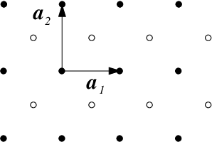
Depending on the dimensionless distance between the plates
| (2.1) |
five distinct bilayer Wigner structures were detected by numerical simulations [29, 30, 31, 32, 33, 34, 35]. In this paper, we study such intervals of -values where the staggered rectangular structures I–III prevail, see Fig. 1. A single layer of these structures corresponds to a rectangular lattice with the aspect ratio , defined by the primitive translation vectors
| (2.2) |
The lattice spacing is determined by the electroneutrality condition that the surface charge of a rectangle must compensate the charge of just one particle per rectangle. The identical structures on the two plates are shifted with respect to one another by a half period . The position vectors of the particles on the Wigner rectangular structure at plate will be denoted by
| (2.3) |
where run over all integers; the particle assignment is obvious. Similarly, the position vectors of the particles on the Wigner rectangular structure at plate are denoted by
| (2.4) |
where run again over all integers. Structure I with arises naturally in the single-layer limit which is known to be characterized by a hexagonal (equilateral triangular) lattice. The aspect ratio is from the interval for soft structure II and for structure III, i.e. the staggered square lattice. The phase transformation I–II, which is not a phase transition, takes place just at [34, 36] or, in other words, structure I exists only at . The phase transition between structures II and III at is of second order, with singularities of mean-field type [36]. Phase III has the lowest energy up to .
For all three structures I-III, the energy per particle, , is expressed as the lattice summation (6.1) in section A of the Supplementary Information. Writing
| (2.5) |
and using techniques introduced in Ref. [36], the function can be written as an integral over certain products of Jacobi theta functions, see Eq. (6.3), and subsequently as an infinite series of the generalized Misra functions
| (2.6) |
see Eq. (6.5). Note that the ordinary Misra functions correspond to [37]. The first few generalized Misra functions with half-integer -indices are expressed in terms of the complementary error function in Eq. (6.7) of section B in the Supplementary Information. This permits us to use very effectively symbolic softwares. The series in generalized Misra functions are rapidly converging; for the well known case of the hexagonal lattice with , the truncation of the series over at reproduces the exact value of the Madelung constant up to decimal digits, respectively [36]. In the present calculations, to keep a high accuracy of the results we truncate the series of the generalized Misra functions at . The evaluation of a series takes a fraction of second of CPU on a standard PC.
For a given dimensionless inter-plate distance , the actual value of the aspect ratio is determined by the energy minimization condition
| (2.7) |
This condition determines the dependence where the lower index means “in the ground-state” or, equivalently, at infinite coupling.
III Monte Carlo simulations
Let the system be in thermal equilibrium at some inverse temperature . There are two relevant length scales at nonzero temperature. The Bjerrum length is the distance at which two unit charges interact with thermal energy . The potential energy of a unit charge at distance from an isolated wall with the surface charge density is equal to . The unit charge has the potential energy equal to thermal energy at distance from the wall
| (3.1) |
known as the Gouy-Chapman length. Since this length is the relevant scale in the direction perpendicular to the surfaces of the two walls, the coordinate will be usually expressed in units of , . The dimensionless coupling parameter , quantifying the strength of electrostatic correlations, is defined as the ratio
| (3.2) |
The SC regime corresponds to either “low temperatures”, large surface charge densities, or equivalently small dielectric constant. The lattice spacing of the Wigner structure , which is the characteristic length scale in the longitudinal plane, is much larger than in the SC regime, .
MC simulations were carried out in a quasi-2D slab geometry for coupling parameters ranging between and , where 512 point charges were confined between two uniformly charged and flat surfaces, each with a surface charged density of , at various fixed separations . The system was periodic in all directions with an extra vacuum slab in the -direction perpendicular to the surfaces and between the slab images. This set-up allowed us to use standard 3D Ewald summation techniques to handle the long-ranged electrostatic interactions, with only minor re-adaptions to correct for the quasi-2D-dimensionality and extra vacuum space [56, 57]. We verified that our vacuum slab is sufficiently wide (typically much wider than the separation between the walls) so as not to influence the results. New MC configurations were either generated by trial displacement of the point charges or by volume preserving floppy-box moves. Two floppy-box moves were utilized: shear or combined biaxial compression/decompression (compression along one axis and decompression along the other such to preserve the box volume). Both deformations were performed in the -plane. All trial move parameters were set such that they each had an acceptance ratio of around 25-40%.
Pressures were estimated across the mid-plane and were collected over Monte Carlo cycles for a given separation and . We applied block averaging of ten blocks to estimate the errors in pressures. A Monte Carlo cycle consisted of either of 512 trial displacement of the point charges or a floppy-box move. Crystal structures were identified both by single configuration snapshots and ensemble averaged 2D-pair correlation maps (of the whole space, of each individual half-space, and across the half-spaces) in the -plane.
We found by numerical simulations that at finite coupling the particles form crystal of type I-III with the aspect-ratio parameter which depends on both the coupling constant and the interplate distance , i.e., . The lattice parameter was obtained by finding the positions of the first two peaks of the 1D-pair correlation functions (ensured that they indeed form crystal structures) where only nearest neighbours, identified by a Delaunay triangulation, been accounted for. The lattice parameter was then taken as the ratio between these two peak positions. Once the lattice parameter reaches unity it is not possible to extract it by this method as the two peaks coalesce to one peak, here we rely instead of inspection of both the 2D- and 1D-pair correlation functions as well as single configuration snapshots to indeed verify that we had square structures (i.e., ). Crystal structures could be identified for all studied ’s only for the largest . only gave crystal structures for . This is consistent with previous numerical results [58, 59, 60] which predict 2D crystallization at any for coupling parameters above and crystallization at contact () above . The factor of two between both thresholds stems from the fact that at , the two layers merge into one, with a double surface charge.
IV Large-coupling description of the crystal phase
For a bilayer Wigner crystal, experiments [59] and simulations [60] give the estimate for melting. This behavior follows from the restricted model in which counterions move only within the 2D Wigner single-layers. In this part, we shall consider to be large enough to localize particles near their Wigner-crystal positions. In our model, as soon as is non divergent (finite ), the particles are not constrained to the wall surfaces and can move in the whole slab domain . Within the canonical ensemble, the relevant thermodynamic quantities are the partition function and the corresponding (dimensionless) free energy per particle defined, up to some irrelevant constants due to the background-charge density, as follows
| (4.1) |
where is the Coulomb interaction energy of the particles and stands for the thermal de Broglie wavelength. We recall that the electric potential induced by the symmetrically charged plates is equal to 0 between the plates. The mean particle number density at point is defined as , where means the statistical average over the canonical ensemble. It fulfills the sum rule . For our particle density which depends only on the perpendicular -coordinate, , this sum rule reduces to the electro-neutrality condition . The particle number density will be considered in a rescaled form
| (4.2) |
in terms of which the electro-neutrality condition takes the form
| (4.3) |
IV.1 Harmonic expansion
The usual large-coupling approach to the counterion system between symmetrically charged plates is to make a harmonic expansion of particle coordinates around their Wigner bilayer positions [31]. We found by numerical simulations that such an approach is not fully adequate and one should assume that at non-infinite coupling, the particles form another reference crystal of type I-III with the aspect-ratio parameter depending, besides the inter-plate distance as it was in the ground state, also on the coupling constant : . In particular, the previously calculated infinite-coupling result in Refs. [31, 32, 34, 36] corresponds to . We aim at performing the harmonic expansion of particle coordinates around this reference crystal, evaluate the corresponding free energy and determine the -parameter of the reference crystal subsequently by minimizing the free energy with respect to . At finite coupling, the particles fluctuate around sites of the reference Wigner crystal, but as soon as the system is in its crystal phase, the particle are localized close to these sites and the reference crystal is not an auxiliary theoretical construction, but its parameters are clearly visible in numerical experiments.
Performing an expansion of the Coulombic energy up to quadratic order in particles displacements, we show in section C.1 of the Supplementary Information that
| (4.4) |
with
| (4.5) |
Here, the prefactor of the linear terms in or reads
| (4.6) | |||||
The quantities and are given by Eqs. (6.16), (6.17) and (6.18), while the Jacobi theta function is defined as (see the Supplementary Information where is also required).
The particle coordinates , and are decoupled within the harmonic expansion of the energy change (4.5). Within the present formalism, the particles have a well defined appurtenance to plate or in the Wigner bilayer. The leading term in the -subspace is linear in for particles and in for particles , with the prefactor function depending on and . This effective electric one-body potential subsumes the effects of the uniform surface charges on the two plates and the particle layer on the opposite plate, while particles on the same plate contribute to higher-order quadratic terms. In the limit of small inter-plate distance , we have
| (4.7) |
i.e. each particle feels the zero potential coming from the uniform surface charge densities on the two plates while the effect of the opposite particle layer with the lattice spacing is negligible; this description coincides with the standard one-body SC fugacity approach for two symmetrically charged plates at small distances [42, 43, 44]. In the large distance limit we have
| (4.8) |
i.e. each particle feels the linear electrostatic potential, or , coming from the surface charge at its own plate; at large distances the discrete counterion structure on the opposite plate is seen as a charge continuum neutralized by the opposite background charge on that plate. In this way the -function describes correctly a continuous interpolation from a two-plate picture at to a one-plate picture at . The contribution of quadratic terms in , which becomes negligible in comparison with the one-body ones in the SC limit , will be treated perturbatively for large . The quadratic terms in the -plane reflect strong particle correlations/repulsions in this plane. Due to the strong particle repulsions, it is reasonable to constrain the particle coordinates within one elementary cell, i.e.
| (4.9) |
The partition function (4.1), with the particle interaction energy given by Eqs. (4.4) and (4.5), factorizes into
| (4.10) |
where
| (4.11) | |||||
| (4.12) | |||||
| (4.13) |
From now on we shall automatically neglect irrelevant terms which do not depend on and . The free energy per particle is given in the harmonic approximation by
| (4.14) |
IV.2 Thermodynamics
Obtaining the partial partition functions , and is a non-trivial task, performed in section C.2 in the Supplementary Information. It relies on the diagonalization of the inverse variance-covariance matrices of fluctuations in the , , and coordinates, which is achieved by means of a 2D Fourier transform. The resulting free energy per particle is expressible in the harmonic approximation as
| (4.15) |
The leading WSC term reads as
| (4.16) | |||||
where the functions and are given by Eqs. (6.40) and (6.45). The prefactor function to the first correction is given by Eqs. (6.23)-(6.24). All quantities in the above formulas are expressed as fast converging series of generalized Misra functions. This means that the thermodynamics can be treated on the same footing as the ground-state energy, at least in the harmonic approximation.
According to the principle of minimum free energy, the aspect ratio of the rectangular lattice is fixed by the condition
| (4.17) |
which provides the explicit dependence of on the coupling constant and the plate distance , . Compare this relation with its ground-state counterpart Eq. (2.7) which reflects an analogous minimization of the interaction energy.
The pressure exerted on the plates can be obtained via the thermodynamic route as follows
| (4.18) |
Rescaling the pressure in the same way as the particle density in (4.2), we get
| (4.19) |
The positive/negative sign of the pressure means an effective repulsion/attraction between the charged walls.
IV.3 Particle density profile and pressure
To find the particle density, we add to each particle in the Hamiltonian the generating (source) one-body potential which will be set to 0 at the end of calculations. The partition function (4.1) is then transformed to
| (4.20) |
and it is a functional of the generating Boltzmann weight . The particle density at point is then obtained as the functional derivative:
| (4.21) |
We show in the Supplementary Information that the (rescaled) particle density takes the WSC expansion form
| (4.22) |
with the leading WSC order
| (4.23) |
This leading WSC particle density has the correct reflection symmetry and satisfies the expected normalization condition
| (4.24) |
The first correction to the particle density is given in Eq. (6.54). Note that The same property holds also in higher WSC orders, so that the electroneutrality condition (4.3) is ensured on the leading WSC order (4.24).
Invoking the contact theorem for planar walls [61, 62], we obtain the pressure as
| (4.25) |
Writing the WSC expansion for the “contact” pressure as , we have in the leading order
| (4.26) |
The first correction is given in section C.3 of the Supplementary Information.
Since for it is simple to show that the expansion coefficients and vanish in the asymptotic large-distance limit, as they should. The thermodynamic and contact pressures must coincide in an exact theory. In an approximate theory like ours, the difference between the two pressures indicates the accuracy of the approach.
IV.4 Comparison with numerical results

We compare the results of our WSC theory with MC data for two values of the coupling constant, namely for large when the system is in its crystal phase and small when the system behaves as a fluid. The distance dependence of the aspect ratio of the rectangular lattice is pictured in Fig. 2. The ground-state case () is represented by the blue curve. The results of the WSC theory are shown by the black curve for and by the red curve for ; note that on the scale of our graph the results of the leading order and the leading order plus the first correction are indistinguishable. In contrast to the ground state with phase I () occurring only at [34, 36], phase I exists in a finite interval of : up to for and up to for . The second-order phase transition between phases I and II is of mean-field type, with the order parameter. The MC data for are represented by open circles. They agree qualitatively with our theoretical results, namely phase I is dominant up to . For the smaller coupling constant , the -range where the structures I-II (and also III) prevail increases; in MC simulations, we did not identify any crystal phase and the counterion system behaves as a fluid. In the inset of Fig. 2, we plot the two theoretical curves and MC data for versus ; we see that the two theoretical curves differ much from one another in this representation. We recall here that the connexion between both scales reads .


The distance dependence of the pressure is presented in Fig. 3 for the coupling constant . The left panel corresponds to the leading WSC order, the right panel presents the results of the leading WSC order plus the first correction. The MC data are indicated by open circles. The WSC results obtained by the thermodynamic route and by the contact theorem are represented by the dashed and solid curves, respectively. It is seen that data obtained by the two methods are very close to one another, and to the MC measures. The location and the value of the pressure minimum is determined especially well by the WSC theory including the first SC correction (see the insets). A very good coincidence with the MC data lasts up to extremely large values of , corresponding to , well beyond the validity of the standard fugacity [42, 43, 44] and Wigner-crystal [46] SC approaches. The analogous plots of versus for the intermediate value of the coupling constant are presented in Fig. 4. In spite of the fact that the counterion system is in the fluid state for this value of , the analytic results agree surprisingly well with MC data. A similar conclusion holds at even smaller values, see section VI where we present data at . This points to the fact that what is relevant is not so much the detailed ionic configuration, but that it is strongly modulated. This gives support to the idea of a correlation hole, developed in section V.


At , some representative particle density profiles are pictured in Fig. 5. The MC data are indicated by open circles. The density profiles obtained in the leading WSC order, see Eq. (4.23), and with the first correction included, see Eqs. (4.22) and (6.55), are represented by the dashed and solid curves, respectively. The logarithmic plots in the insets illustrate that in the large interval of the present WSC theory predicts contact particle densities and the slopes of the density profile close to the walls which are in excellent agreement with MC data. This shows the relevance of the idea of an effective local field (an effective one-body potential), embodied in , which depends on the distance and on the geometry of the ionic arrangement, together with the accuracy of our approach for computing this non-trivial quantity. Besides, it is noteworthy that for the considered extremely large coupling constant, the inclusion of the correction to the leading WSC order improves substantially the results. For small distances and , the WSC density profiles agree with MC in the whole inter-plate slab, but with increasing there is a discrepancy between the WSC and MC results in the middle region between the walls characterized by extremely small particle densities.
V Strong-coupling theory for the fluid phase
The Wigner bilayer is stable at very large values of the coupling constant. For intermediate and small values of , the counterion system behaves as a fluid which is isotropic along the plane. The strong Coulomb repulsion leads to a depletion region around each particle, inaccessible to other particles, known as the correlation hole [25, 40, 52, 45, 53, 54].
Within the WSC theory, the Wigner structure in the plane underlies the calculation of the crucial effective local field , see Eq. (4.6). It determines the slope of the density profile close to the wall. To describe physically the fluid regime, the idea is to substitute the lattice representation of by its continuum counterpart, with a radial cut of the lattice summation at small distances due to the correlation hole. In particular, rewriting the lattice sum as
| (5.1) |
and regarding that there is surface per site on the Wigner lattice, we can express (5.1) as a continuum integral in the following way
| (5.2) |
To estimate the short-distance cut , i.e. the radius of the correlation hole around the reference particle, one has to realize that the reference particle on plate 1 is in the center of an elementary cell of the particle crystal on plate 2. Let us choose the symmetric square lattice, and apply the Voronoi construction of the Wigner-Seitz primitive cell which has surface . Thus, and we end up with
| (5.3) |
This fluid version of the -function has the correct limiting values for and for . We shall refer to this correlation-hole theory to as ch1.
Another phenomenological way to express the functional dependence of combines geometrical features, overall electroneutrality together with space fluctuations of charged particles in the fluid regime. We substitute the crystal bilayer structure by a couple of correlation holes with respect to a reference particle, which appertains say to plate 1. We thereby obtain one disk of radius at plate 1 and the other disk of radius at plate 2. Particles are smeared out on the plate regions outside of the correlation-hole disks; the corresponding “punctuated” planes are therefore taken as neutral. The charge of the reference particle must be compensated by the total surface charge on the disks which implies the constraint
| (5.4) |
The disk radiuses depend on the distance between the plates, and . If the two walls touch each other, , the correlation holes around the reference particle are the same on both sides, i.e.,
| (5.5) |
The plate-1 and plate-2 subspaces decouple at asymptotically large distances . From the point of view of the reference particle (attached to plate 1), the hole at plate 2 disappears due to thermal fluctuations of charged particles at plate 2, , while the charge conservation rule leads to an increase of the radius of the hole at plate 1: , like in the one-plate geometry. Respecting the constraint (5.4), the two limits are matched by the phenomenological interpolation formulas
| (5.6) |
where defines a crossover scale. For simplicity we set . For the reference particle at distance from plate 1 and at distance from plate 2, the electrostatic energy yielded by the two correlation holes is given by
| (5.7) | |||||
Within the single-particle picture, we can take the whole one-body Boltzmann factor or restrict ourselves to the linear term in the energy, , with
| (5.8) |
This coincides with the geometrical one (5.3) at small distances ; it furthermore shares with ch1 the correct limiting value 1 at . We shall refer to this correlation-hole theory to as ch2.

The dependences of different variants of the function on are pictured in Fig. 6. The crystal versions of with the extreme values of the aspect ratio and are represented by the black solid and dashed curves, respectively. The blue solid and dotted-dashed curves correspond to the correlation-hole ch1 formula (5.3) and the ch2 formula (5.8), respectively. Note that the four plots are relatively close to each other, which documents the robustness of the method.


Having an expression for the fluid , the leading SC estimate for the density profile is given by Eq. (4.23) and the pressure can be obtained by using the contact formula (4.26). For an intermediate coupling constant , the plot of the rescaled pressure on is pictured in the left panel of Fig. 7. We see that the results of our two correlation-hole approaches ch1 and ch2, represented respectively by the dashed and solid curves, are close to the MC data (open circle symbols). For the relatively small value of the coupling constant , the analogous plot is presented in the right panel, with again a fair agreement.


The density profiles for at the four distances between the walls , , and are pictured in Fig. 8. MC results are compared to the WSC predictions (with and without the first correction) as well as to the two correlation hole theories. A conclusion that emerges is that while all approaches proposed yield acceptable quantitative results, the Wigner SC method is the most accurate. This is somewhat surprising since we sit here in a coupling-range where no crystal is formed. Yet, accuracy requires that the correction is included, and it stems from a rather demanding analytical work. Here, a fair assessment of ch performance would be to compare to WSC without correction, in which case ch is quite superior.
VI Conclusion
The aim of this paper was to construct a strong-coupling theory for thermal equilibrium of pointlike counterions between parallel and symmetrically charged plates. The goal was to extend significantly the range of interplate distances where a trustworthy analytical effective force is available. This range was hitherto reduced to smaller than a couple of Gouy-Chapman lengths [44, 46], meaning of order unity. To this end, we studied the counterion system in both the crystal phase at extremely large Coulombic couplings and in the fluid phase, at large and intermediate couplings.
A new type of the Wigner SC theory of the crystal phase is proposed in Sec. IV, in a perturbative fashion. At infinite coupling, the counterions stick to the plate surfaces and as increases from 0, they form successively bilayer Wigner crystals of rectangular type with the aspect ratio decreasing from (hexagonal monolayer coined I) to 1 (staggered square structure III), see Fig. 1. At finite couplings, our MC simulations indicate that counterions are still localized around sites of a bilayer structure where depends, besides distance , also on the coupling constant . In particular, structure I with , which exists only at in the ground state, prevails in a nonzero interval of values for finite couplings, see open circles in Fig. 2. We thus constructed a Wigner-type SC theory based on a harmonic expansion of particle coordinates around the sites of the Wigner bilayer, with a free aspect ratio , fixed at the end of calculations by minimizing the free energy. Two variants of the WSC expansion were obtained. The leading-order one is characterized by an effective one-body potential where the prefactor function , which is -dependent, vanishes for (two-plates problem at small distance) and goes to unity for (two separated one-plate problems). The second variant involves the first correction term and, in general, improves substantially the results of the leading-order version, even for extremely large coupling constants. We have reported a good agreement with Monte Carlo simulation results, be it for the interplate pressure, or for the ionic density profiles. This is the case, expectedly, at very large coupling parameters, where the system becomes a (bilayer) Wigner crystal as assumed in our treatment. Yet, the predicted pressures and profiles also appear to be reliable at much smaller values, where crystals are completely melted. We illustrate this point in Fig. 9, where and , well below the coupling constant of the crystal-fluid transition ( on the order of 30 000).


Guided by the structure of the WSC results, we also derived a strong-coupling description of the fluid regime in Sec. V. Here, the lattice representation of the effective field is replaced by the continuum one based on the idea of a correlation hole, that has already proven useful in related contexts [54, 55]. We proposed two phenomenological constructions of , with the results (5.3) and (5.8); the corresponding correlation-hole theories were coined as ch1 and ch2. As is seen in Fig. 6, the approximate plot of on distance depends only slightly on the choice of the correlation-hole theory, and ends up close to the WSC derivation. The correlation hole program leads to observables like pressure and densities that fare reasonably against numerical simulations. Fig. 9 shows that the ch2 form (slightly better for the chosen couplings than ch1), performs as well as the WSC method, while its effective field is simpler to compute (compare Eqs. (4.6) and (5.8)). This completes our goal, since our approach allows to reach distances (in Gouy-Chapman units) of order , i.e. the typical scale of inter-ionic distance. To put it differently, no analytical theory could so far account for the increasing part of the pressure profile (see e.g. Fig. 9, or the other pressure plots in this paper) after the pressure minimum. Previous theories [44, 46] did only describe well the decreasing branch of the pressure curve, located at smaller separations. We recall that the large-distance regime is accounted for by the PB mean-field theory. The latter is repulsive, meaning that the pressure should vanish at a specific large but finite distance, a phenomenon that is particularly difficult to study analytically, and beyond our scope here.
In our treatment, we considered as eligible WSC structures rectangle types of phases only. As is seen in Fig. 2, the decrease of the coupling constant increases the -range where the structures I-II (and also III) prevail. In the ground state, at intermediate to large distances, two different structures (staggered rhombic, so-called structure IV, and staggered hexagonal, structure V) were also observed. These candidates a priori impinge on the large-distance WSC calculations (i.e. for value of order unity and beyond), but presumably in a modest way. Finally, future plans include extending the present SC methods to asymmetrically charged planes and to ions having some structure, starting with a hard core. A difficulty for the former problem lies in the extreme complexity of the ground-state phase diagram [38]. Another venue concerns the inclusion of salt (microions with charges of both signs).
Acknowledgements.
We would like to dedicate this work to the memory of Per Linse who was a true expert in both electrostatics and computer simulations. M.T. especially wants to honor Per Linse for having been a great teacher and a dear colleague, who always showed a genuine interest in other people’s work. This work was supported by the Grant VEGA No. 2/0003/18 and by the European Union’s Horizon 2020 research and innovation programme under ETN grant 674979-NANOTRANS. M.T. acknowledges financial support by the Swedish Research Council (621-2014-4387).Supplementary material for “Strong-coupling theory of counterions between symmetrically charged walls: from crystal to fluid phases”
We present below some results from previous work for self-containedness (sections A and B), and calculations explaining the results presented in the main text (sections C and D). Section C reports the bulk of our analysis. We start by ground state features, before working out the harmonic expansion treatment leading to the free energy in the crystal phase, from which thermodynamic properties and ionic profiles follow.
A Series representations of the ground-state energy
Taking the particle at point of plate 1 as a reference, the Coulomb interaction energy per particle of structures I-III can be written as
| (6.1) |
where the first sum corresponds to the interactions with particles on the same plate 1 and the second sum with particles on plate 2. The background term cancels an infinite constant due to the slow decay of the Coulomb potential at large distances.
The energy can be reexpressed in terms of a rapidly converging series by using the method presented in Ref. [36]. We rewrite the ground-state energy per particle as in Eq. (2.5). First, using the gamma identity
| (6.2) |
( denotes the Gamma function) with , the -function is expressed in terms of Jacobi theta functions with zero argument [64] and as follows
| (6.3) | |||||
Here, the effect of the background charge density on the plates is to subtract the singularity of the product of theta functions as . Using the Poisson summation formula
| (6.4) |
one can reduce the integration support to . Applying then once more the Poisson summation formula, the -function can be expressed as a series in the generalized Misra functions (2.6):
| (6.5) | |||||
B Generalized Misra functions
C Large-coupling description of the crystal phase
C.1 Harmonic expansion of the energy
Starting from a crystalline configuration, let us shift each particle at plate from its reference Wigner-lattice position (2.3) to
| (6.9) |
where the coordinate shifts , and are assumed to be small. Similarly, we shift the Wigner position (2.4) of each particle at plate to the one
| (6.10) |
where now , and are assumed to be small.
If the particles and are localized on the same plate, either or , the change of the Coulomb energy due to the particle shifts reads as
| (6.11) |
If both particles are at plate , the expansion of in small deviations , and is straightforward. Since , the same holds for two particles being at plate where the deviations and are small. If particles and belong to different plates, say and , the energy change is given by
| (6.12) | |||||
In this case, we write and perform the expansion of the energy change in the small quantities and . The total energy is expressible as
| (6.13) |
Within the harmonic approximation, we expand every up to quadratic terms in small deviations, supposing that the ratios , , are small variables for particles and that , , are small variables for particles . Many terms disappear because of the symmetry of the energy with respect to the reflection transformations and . The final result for the energy change is Eq. (4.5) in the main text:
| (6.14) |
with
| (6.15) | |||||
The quantity involves all terms quadratic in variables if and if ,
| (6.16) | |||||
and the expansion coefficients in the -plane are given by
| (6.17) |
if particles and belong to the same plate and by
| (6.18) |
if particles and belong to different plates.
C.2 Thermodynamics
To express as a perturbative series in , we introduce the counterpart of (4.11) for non-interacting particles in the external potential only:
| (6.19) |
We have
| (6.20) |
where denotes the statistical averaging over the system of non-interacting particles defined by the partition sum . The quantity can be written as the cumulant expansion:
| (6.21) |
where each term of the expansion is extensive, i.e. proportional to the particle number . Restricting ourselves to the lowest cumulant order, we obtain
| (6.22) |
with . The evaluation of yields:
| (6.23) | |||||
where corresponds to the lattice sum
| (6.24) |
and the one-body averages
| (6.25) |
In particular, we shall need
| (6.26) | |||||
| (6.27) |
To calculate the integral in (4.12), we respect the -coordinate constraint (4.9) and rescale the particle -coordinates by the factor to obtain
| (6.28) |
where goes to infinity in the large- limit. Here, going back to dimensioned lengths, a new relevant length scale arises, . It is readily checked that it measures the amplitude of in plane -fluctuations around a lattice position. Incidentally, we note first that a similar scaling arises for the minimum of the pressure curves, in the regime of like-charge attraction, that is largely met here [25, 46]. Second, this provides a new light on the melting criterion alluded to above, where the critical coupling in the 2D-confined problem is around 15000. This yields , a value close to Lindeman type of criteria [63]. To avoid the divergence of the consequent integral manifesting itself by the invariance of with respect to a uniform coordinate shift , we shall make provision for finiteness of the -bound for a large but finite and ignore the zero Fourier mode, see below. Omitting in (6.28) irrelevant prefactors we end up with the integral of Gaussian type
| (6.29) |
where the -matrix is defined by
| (6.30) |
According to Fig. 1, within the plane we can represent the Wigner bilayer as the regular 2D lattice of alternating white (belonging to plate ) and black (belonging to ) points, with the primitive translation vectors
| (6.31) |
and the surface of the elementary cell . The matrix elements depend only on the distance of lattice points and therefore is an circulant matrix with known eigenvalue spectrum. Let us define the 2D Fourier transform of any lattice function as follows
| (6.32) |
where the vectors belong to the first Brillouin zone (BZ) of the reciprocal lattice with the primitive vectors , defined by the relations
| (6.33) |
In particular,
| (6.34) |
and the surface of the BZ is given by . Since the with are the eigenvalues of the matrix , we have
| (6.35) |
the zero-mode being excluded. In the thermodynamic limit , the -vectors cover uniformly the BZ defined by the primitive vectors (6.34) and we can write
| (6.36) | |||||
Consequently,
| (6.37) |
Now we want to express appropriately the Fourier component , the elements of the -matrix being defined in terms of those of the -matrix [see formulas (6.17) and (6.18)] in Eq. (6.30). We introduce the auxiliary Fourier lattice functions
| (6.38) | |||||
| (6.39) |
Note that the previous lattice sum (6.24) is expressible as . The Misra series representations of and are given in Eqs. (6.61) and (6.62) in section D, respectively. Introducing the function
| (6.40) | |||||
it holds that
| (6.41) |
C.3 Particle density profile and pressure
We start from
| (6.46) |
a functional of the generating Boltzmann weight , such that
| (6.47) |
For our -dependent density one can ignore harmonic modes along the plane as well as -independent terms. After simple algebra, we find that
| (6.48) |
where the functional is given by Eq. (6.23) with the moments redefined as follows
| (6.49) |
Then the (rescaled) particle density can be represented as the WSC expansion
| (6.50) |
Since
| (6.51) |
and , we have in the leading WSC order
| (6.52) |
The first correction to the particle density is generated from by using the functional derivatives of the moments
| (6.53) | |||||
| (6.54) |
In particular,
| (6.55) | |||||
Because of the equalities
| (6.56) |
we have
| (6.57) |
so that the electroneutrality condition is met.
Finally, the contact theorem for planar walls [61] relates the total contact density of particles on the wall and the pressure. Within our notation, it is expressible as
| (6.58) |
Writing the WSC expansion for the “contact” pressure as , we get
| (6.59) |
and the first correction reads as
| (6.60) | |||||
D Series representations of certain lattice functions
References
- [1] T. Palberg, M. Medebach, N. Garbow, M. Evers, A. Barreira Fontecha, H. Reiber, and E. Bartsch, J. Phys.: Condens. Matter 16, S4039 (2004).
- [2] Ph. Attard, Adv. Chem. Phys. 92, 1 (1996).
- [3] J.P. Hansen and H. Löwen, Annu. Rev. Phys. Chem. 51, 209 (2000).
- [4] Y. Levin, Rep. Prog. Phys. 65, 1577 (2002).
- [5] R. Messina, J. Phys.: Condens. Matter 21, 113102 (2009).
- [6] A. Khan, B. Jönsson, and H. Wennerström, J. Chem. Phys. 89, 5180 (1985).
- [7] R. Kjellander, S. Marčelja, and J. P. Quirk, J. Colloid Interface Sci. 126, 194 (1988).
- [8] V. A. Bloomfield, Biopolymers 31, 1471 (1991).
- [9] D. C. Rau and A. Pargesian, Biophys. J. 61, 246 (1992); ibid. 61, 260 (1992).
- [10] P. Kékicheff, S. Marčelja, T. J. Senden, and V. E. Shubin, J. Chem. Phys. 99, 6098 (1993).
- [11] M. Dubois, T. Zemb, N. Fuller, R. P. Rand, and V. A. Pargesian, J. Chem. Phys. 108, 7855 (1998).
- [12] L. Gulbrand, B. Jönsson, H. Wennerström, and P. Linse, J. Chem. Phys. 80, 2221 (1984).
- [13] R. Kjellander and S. Marčelja, Chem. Phys. Lett. 112, 49 (1984).
- [14] D. Bratko, B. Jönsson, and H. Wennerström, Chem. Phys. Lett. 128, 449 (1986).
- [15] N. Grønbech-Jensen, R. J. Mashl, R. F. Bruinsma, and W. M. Gelbart, Phys. Rev. Lett. 78, 2477 (1997).
- [16] P. Linse and V. Lobaskin, Phys. Rev. Lett. 83, 4208 (1999).
- [17] P. Linse and V. Lobaskin, J. Chem. Phys. 112, 3917 (2000).
- [18] V. A. Bloomfield, Curr. Opin. Struct. Biol. 6, 334 (1996).
- [19] S. May, A. Iglic, J. Rescic, S. Maset, and K. Bohinc, J. Phys. Chem. B 112, 1685 (2008).
- [20] Y. W. Kim, J. Yi, and P. A. Pincus, Phys. Rev. Lett. 101, 208305 (2008).
- [21] V. Lobaskin and P. Linse, J. Chem. Phys. 111, 4300 (1999).
- [22] D. Andelman, in Soft Condensed Matter Physics in Molecular and Cell Biology, edited by W.C.K. Poon and D Andelman (Taylor & Francis, New York, 2006).
- [23] Ph. Attard, D. J. Mitchell, and B. W. Ninham, J. Chem Phys. 88, 4987 (1988); 89, 4358 (1988); R. Podgornik, J. Phys. A 23, 275 (1990); R. R. Netz and H. Orland, Eur. Phys. J. E 1, 203 (2000).
- [24] B. I. Shklovskii, Phys. Rev. E 60, 5802 (1999); Phys. Rev. Lett. 82, 3268 (1999).
- [25] Y. G. Chen and J. D. Weeks, Proc. Natl. Acad. Sci. U. S. A. 103, 7560 (2006); J. M. Rodgers, C. Kaur, and Y. G. Chen, Phys. Rev. Lett. 97, 097801 (2006).
- [26] A. P. dos Santos, A. Diehl, and Y. Levin, J. Chem. Phys. 130, 124110 (2009).
- [27] M. Baus and J.-P. Hansen, Phys. Rep. 59, 1 (1980).
- [28] S. Earnshaw, Trans. Cambridge Philos. Soc. 7, 97 (1842).
- [29] V.I. Falko, Phys. Rev. B 49, 7774 (1994).
- [30] K. Esfarjani and Y. Kawazoe, J. Phys.: Condens. Matter 7 7217 (1995).
- [31] G. Goldoni and F.M. Peeters, Phys. Rev. B 53, 4591 (1996).
- [32] I. V. Schweigert, V. A. Schweigert, and F. M. Peeters, Phys. Rev. Lett. 82, 5293 (1999); Phys. Rev. B 60, 14 665 (1999).
- [33] J. J. Weis, D. Levesque, and S. Jorge, Phys. Rev. B 63, 045308 (2001).
- [34] R. Messina and H. Löwen, Phys. Rev. Lett. 91, 146101 (2003); E. C. Oǧuz, R. Messina, and H. Löwen, Europhys. Lett. 86, 28002 (2009).
- [35] V. Lobaskin and R. R. Netz, Europhys. Lett. 77, 38003 (2007).
- [36] L. Šamaj and E. Trizac, Europhys. Lett. 98, 36004 (2012); Phys. Rev. B 85, 205131 (2012).
- [37] R. D. Misra, Math. Proc. Cambridge Philos. Soc. 36, 173 (1940); M. Born and R. D. Misra, Math. Proc. Cambridge Philos. Soc. 36, 466 (1940).
- [38] M. Antlanger, G. Kahl, M. Mazars, L. Šamaj, and E. Trizac, Phys. Rev. Lett. 117, 118002 (2016).
- [39] L. Šamaj and E. Trizac, Contrib. Plasma Phys. 52, 53 (2012); Europhys. Lett. 100, 56005 (2012).
- [40] I. Rouzina and V. A. Bloomfield, J. Phys. Chem. 100, 9977 (1996).
- [41] V. I. Perel and B. I. Shklovskii, Physica A 274, 446 (1999).
- [42] A.G. Moreira and R.R. Netz: Europhys. Lett. 52, 705 (2000); Phys. Rev. Lett. 87, 078301 (2001).
- [43] R.R. Netz: Eur. Phys. J. E 5, 557 (2001).
- [44] A.G. Moreira and R.R. Netz: Eur. Phys. J. E 8, 33 (2002).
- [45] C. D. Santangelo, Phys. Rev. E 73, 041512 (2006).
- [46] L. Šamaj and E. Trizac, Phys. Rev. Lett. 106, 078301 (2011); Phys. Rev. E 84, 041401 (2011).
- [47] M. Kanduč and R. Podgornik, Eur. Phys. J. E 23, 265 (2007); Y. S. Jho, M. Kanduč, A. Naji, R. Podgornik, M. W. Kim, and P. A. Pincus, Phys. Rev. Lett. 101, 188101 (2008).
- [48] M. Kanduč, M. Trulsson, A. Naji, Y. Burak, J. Forsman, and R. Podgornik, Phys. Rev. E 78, 061105 (2008).
- [49] F. Paillusson and E. Trizac, Phys. Rev. E 84, 011407 (2011).
- [50] M. Kanduč, A. Naji, J. Forsman, and R. Podgornik, J. Chem. Phys. 132, 124701 (2010); Phys. Rev. E 84, 011502 (2011).
- [51] Y. Burak, D. Andelman, and H. Orland, Phys. Rev. E 70, 016102 (2004).
- [52] S. Nordholm, Chem. Phys. Lett. 105, 302 (1984).
- [53] M. M. Hatlo and L. Lue, EPL 89, 25002 (2010).
- [54] L. Šamaj, A. P. dos Santos, Y. Levin, and E. Trizac, Soft Matter 12, 8768 (2016).
- [55] I. Palia, M. Trulsson, L. Šamaj, and E. Trizac, arXiv:1803.00359, submitted (2018).
- [56] I.-C. Yeh and M. L. Berkowitz, J. Chem. Phys. 111, 3155 (1999).
- [57] M. Mazars, J.-M. Caillol, J.-J. Weis, and D. Levesque, Condens. Matter Phys. 4, 697 (2001).
- [58] H. Boroudjerdi, Y.-W. Kim, A. Naji, R. R. Netz, X. Schlagberger, and A. Serr, Phys. Rep. 416, 129 (2005).
- [59] C. C. Grimes and G. Adams, Phys. Rev. Lett. 42, 795 (1979).
- [60] R. H. Morf, Phys. Rev. Lett. 43, 931 (1979).
- [61] D. Henderson and L. Blum, J. Chem. Phys. 69, 5441 (1978); D. Henderson, L. Blum, and J.L. Lebowitz, J. Electroanal. Chem. 102, 315 (1979); S.L. Carnie, D.Y.C. Chan, J. Chem. Phys. 74, 1293 (1981); H. Wennerström, B. Jönsson, and P. Linse, J. Chem. Phys. 76, 4665 (1982).
- [62] J.-P. Mallarino, G. Téllez, E. Trizac, Mol. Phys. 113, 2409 (2015).
- [63] J.-P. Hansen and I. R. McDonald, Theory of Simple Liquids, Academic Press, Amsterdam (2007).
- [64] I. S. Gradshteyn and I. M. Ryzhik, Table of Integrals, Series, and Products, 6th ed. (Academic, London, 2000).
- [65] I. Travěnec and L. Šamaj, Phys. Rev. E 92, 022306 (2015).