跳到论文正文
W Papers独立论文阅读器 arXiv:1804.08432 论文正文 计算阅读时间 · 0%
引用这篇论文根据当前论文元数据生成,正式投稿前建议核对。


License: arXiv.org perpetual non-exclusive license
arXiv:1804.08432v2 [math.PR] 14 May 2018

Nesting Monte Carlo for high-dimensional Non Linear PDEs

Xavier Warin ††thanks: EDF R&D & FiME, Laboratoire de Finance des Marchés de l’Energie, xavier.warin@edf.fr
Abstract

A new method based on nesting Monte Carlo is developed to solve high-dimensional semi-linear PDEs. Convergence of the method is proved and its convergence rate studied. Results in high dimension for different kind of non-linearities show its efficiency.

1 Introduction

The resolution of Non Linear PDEs in high dimension is a challenging task due to the so-called ”curse of dimensionality”. Deterministic method can’t cope with dimensions higher than 4 even using super-computers. In order to solve problems in higher dimension, effective resolution of Semi-Linear PDEs based on the BSDE approach first proposed by [21] were developed in [16] and [20]. A lot of literature on the subject has developed in recent years and the methodology has been extended to solve full non linear PDEs in [13], [24].
However because the methodology needs some basis functions to project conditional expectation, it faces the curse of dimensionality too by not being able to solve PDEs in dimension higher than six or seven.
Recently two new approaches have emerged in very high dimensions:

  • •

    The first is based on Deep Learning and uses deep neural networks [10], [9], [15]. The method seems to be effective in dimension over 100 but no proof of convergence is currently available and therefore we don’t know its limitations.

  • •

    The second is based on branching methods and is effective for non linearities polynomial in the solution uu and its gradient D​uDu. Convergence results are given in [18] and numerical results show that the PDEs can be solved in dimension 100. However the authors showed that the variance of the method explodes rapidly when the maturity grows or when the non linearity becomes important: numerical tests confirm that it is in fact the case. This methodology has being extended for other non linearities in [4] and [3] and the maturity problem is solved but at the price of the introduction of some grids meaning that the ”curse of dimensionality” is back.

  • •

    The third is developed in [12], [11], [19] with an algorithm based on Picard iterations, multi-level techniques and automatic differentiation permitting to solve some high dimensional PDEs with non linearity in uu and D​uDu. The convergence of the algorithm is given and a lot of numerical examples show its efficiency in high dimension.

As for the branching method, the methodology proposed here is based on the Feynman-Kac representation of the PDEs coupled with the randomization of the time step proposed in [18]. This approach is combined with nesting Monte Carlo with a given depth. Then it is possible to get effective schemes to solve non-linear PDEs.
Because a truncation after a given number mm of nesting is achieved, the method is biased.
For the demonstration of the convergence of the proposed schemes it is possible to follow classical approaches as the one used in [22]. It permits to understand how many particles to use at each nesting level and the number of nesting level mm to take.
Classically the error is composed of a biased term and a variance term. It can be shown than the bias term goes to zero very quickly with mm but to be effective we need to be able to take mm below 5 or 6 such that the nesting Monte Carlo can be used. Therefore, as we will see, a limitation of the method will be that the maturity cannot be too large.

However the methodology proposed here has a lot of good properties :

  • •

    It is very simple to implement,

  • •

    It needs a very low memory to run on computers,

  • •

    Its convergence is independent on the dimension dd of the problem,

  • •

    It is embarrassingly parallel so it can be run easily on super computers,

  • •

    If the different Lipschitz constants associated to the non-linearity are not too large, then the number of particles to take at each level to get a given accuracy is decreasing very fast giving a method very quickly converging.

Practically we will show that the method can be used on a wide set of cases and that we are able for example to solve all test cases proposed in [10], [9] for example.
The article has two parts :

  • •

    The first part is devoted to the resolution of the problem with linearity in uu. The scheme is given, its convergence studied and numerical results in dimension 6 and 100 show the efficiency of the scheme.

  • •

    The second part is devoted to non linearities in D​uDu. Based on automatic differentiation [14], we give a first scheme and show its convergence. We then introduce a second scheme using ideas in [26]. The second scheme permits to gain little theoretically but numerically we show that is is far more effective than the first proposed. We test the methods on problems with dimensions 10 to 100.

In the sequel we use the classical notation for Y∈ℝdY\in\mathbb{R}^{d} , ‖Y‖2=∑i=1dYi2||Y||_{2}=\sqrt{\sum_{i=1}^{d}Y_{i}^{2}}.
Given two matrix A,B∈𝕄dA,B\in\mathbb{M}^{d}, denote A:B:=Trace​(A​B⊤)A:B:=\mbox{Trace}(AB^{\top}), 1​Id1\hskip-2.84526pt{\rm I}_{d} is the unit vector of ℝd\mathbb{R}^{d} and 𝐈d{\bf I}_{d} the identity matrix of 𝕄d\mathbb{M}^{d}.
All numerical experiments are achieved on a cluster using 8 nodes with a total of 224 cores and MPI is used for parallelization. The generation of random numbers is achieved using Tina’s Random Number Generator Library [1]. All computational times are given for a configuration of Intel Xeon CPU E5-2680 v4 2.40GHz (Broadwell).

2 A first non linear case

In this section we study the case of a non linearity in uu and we aim at solving the PDE for t<T,x∈ℝdt<T,~x\in\mathbb{R}^{d}:

(−∂tu−ℒu)(t,x)\displaystyle(-\partial_{t}u-{\cal L}u)(t,x) =f⁡(t,x,u⁡(t,x)),\displaystyle=f(t,x,u(t,x)),
uT\displaystyle u_{T} =g,\displaystyle=g, (1)

where

ℒ​u​(t,x):=μ​D​u​(t,x)+12​σ​σ⊤:D2​u​(t,x),\displaystyle{\cal L}u(t,x):=\mu Du(t,x)+\frac{1}{2}\sigma\sigma^{\top}\!:\!D^{2}u(t,x), (2)

so that ℒ{\cal L} is the generator associated to

X^t=x+μ​t+σ​d​Wt,\displaystyle\hat{X}_{t}=x+\mu t+\sigma dW_{t}, (3)

with μ∈ℝd\mu\in\mathbb{R}^{d}, σ∈𝕄d\sigma\in\mathbb{M}^{d} is some constant matrix and WtW_{t} a dd-dimensional Brownian motion.
We will use the following assumptions:

Assumption 2.1

ff is uniformly Lipschitz in uu with constant KK :

|f⁡(t,x,y)−f⁡(t,x,w)|≤K​|y−w|∀t∈ℝ+,x∈ℝd,(w,y)∈ℝ2.\displaystyle|f(t,x,y)-f(t,x,w)|\leq K|y-w|\quad\forall t\in\mathbb{R}^{+},x\in\mathbb{R}^{d},(w,y)\in\mathbb{R}^{2}. (4)
Assumption 2.2

Equation (1) has a solution u∈C1,2​([0,T]×ℝd)u\in C^{1,2}([0,T]\times\mathbb{R}^{d}), such that

  • •

    uu is θ\theta-Hölder with θ∈(0,1]\theta\in(0,1] in time with constant K^\hat{K} :

    |u⁡(t,x)−u⁡(t~,x)|≤K^​|t−t~|θ∀(t,t~,x)∈[0,T]×[0,T]×ℝd,\displaystyle|u(t,x)-u(\tilde{t},x)|\leq\hat{K}|t-\tilde{t}|^{\theta}\quad\quad\quad\forall(t,\tilde{t},x)\in[0,T]\times[0,T]\times\mathbb{R}^{d},
  • •

    u⁡(t,x)u(t,x) has a quadratic growth in xx uniformly in tt,

In this section ρ⁡(x)=λ​e−λ​x\rho(x)=\lambda e^{-\lambda x} is the density of a random variable with exponential law.
Denote

F¯​(t):=∫t∞ρ⁡(s)​𝑑s=e−λ​t=1−F⁡(t),\overline{F}(t):=\int_{t}^{\infty}\rho(s)ds=e^{-\lambda t}=1-F(t),

so that FF is the cumulative distribution function of a random variable with density ρ\rho.

2.1 Idea of the algorithm

We consider a sequence of i.i.d. random variables (τm)m≥1(\tau_{m})_{m\geq 1} of density ρ\rho.
We consider the sequence defined by:

{T0=0,Tk+1=(Tk+τk)∧T.\left\{\begin{array}[]{lll}T_{0}&=&0,\\ T_{k+1}&=&(T_{k}+\tau_{k})\wedge T.\end{array}\right. (5)

We further define NT=inf{n|Tn+1≥T}N_{T}=\inf\{n|T_{n+1}\geq T\}.
We also consider a sequence of independent dd-dimensional Brownian motion (Wtm)m≥1(W^{m}_{t})_{m\geq 1}, which are independent of (τm)m≥1(\tau_{m})_{m\geq 1}.

Define Wt=Wt1W_{t}=W^{1}_{t} for all t∈[0,T1]t\in\big[0,T_{1}\big] and then for each kk, define

Wt:=WTk+Wt−Tkk+1,for all​t∈[Tk,Tk+1].\displaystyle W_{t}~:=~W_{T_{k}}+W^{k+1}_{t-T_{k}},~~\mbox{for all}~t\in[T_{k},T_{k+1}]. (6)

We define an associated diffusion process (Xt)t∈[Tk,Tk+1](X_{t})_{t\in[T_{k},T_{k+1}]} by means of the following SDE:

Xt=XTk+μ⁡(t−Tk)+σ​Wt−Tkk+1​t∈[Tk,Tk+1],​-a.s.,\displaystyle X_{t}~=~X_{T_{k}}+\mu(t-T_{k})+\sigma W^{k+1}_{t-T_{k}}~~t\in[T_{k},T_{k+1}],~~\lx@paragraphsign\mbox{-a.s.,} (7)

with X0=xX_{0}=x.

Denoting by 𝔼t,x\mathbb{E}_{t,x} the expectation operator conditional on Xt=xX_{t}=x at time tt, from the Feynman-Kac formula the representation of the solution uu valid under assumption 2.2 is given by:

u⁡(0,x)=\displaystyle u(0,x)= 𝔼0,x​[F¯​(T)​g⁡(XT)F¯​(T)+∫0Tf⁡(t,Xt,u⁡(t,Xt))ρ⁡(t)​ρ​(t)​𝑑t]\displaystyle\mathbb{E}_{0,x}\Big[\overline{F}(T)\frac{g(X_{T})}{\overline{F}(T)}+\int_{0}^{T}\frac{f(t,X_{t},u(t,X_{t}))}{\rho(t)}\rho(t)dt\Big]
=\displaystyle= 𝔼0,x​[ϕ⁡(0,T1,XT1,u⁡(T1,XT1))],\displaystyle\mathbb{E}_{0,x}\big[\phi\big(0,T_{1},X_{T_{1}},u(T_{1},X_{T_{1}})\big)\big],
ϕ⁡(s,t,y,z)\displaystyle\phi(s,t,y,z) :=𝟏{t≥T}F¯​(T−s)​g​(y)+𝟏{t<T}ρ⁡(t−s)​f​(t,y,z).\displaystyle:=\frac{{\bf 1}_{\{t\geq T\}}}{\overline{F}(T-s)}g(y)\!+\!\frac{{\bf 1}_{\{t<T\}}}{\rho(t-s)}f(t,y,z).

Recursively we have for n<NTn<N_{T}, noting un=u⁡(Tn,XTn)u_{n}=u(T_{n},X_{T_{n}}) :

un=\displaystyle u_{n}= 𝔼Tn,XTn​[ϕ⁡(Tn,Tn+1,XTn+1,un+1)],\displaystyle\mathbb{E}_{T_{n},X_{T_{n}}}\big[\phi\big(T_{n},T_{n+1},X_{T_{n+1}},u_{n+1}\big)\big], (8)

We further consider the truncated operator after pp switches :

upp=\displaystyle u_{p}^{p}= g⁡(XTp),\displaystyle g(X_{T_{p}}),
unp=\displaystyle u_{n}^{p}= 𝔼Tn,XTnn​[ϕ⁡(Tn,Tn+1,XTn+1,un+1p)],n<p, defined if ​Tn<T\displaystyle\mathbb{E}_{T_{n},X^{n}_{T_{n}}}\big[\phi\big(T_{n},T_{n+1},X_{T_{n+1}},u_{n+1}^{p}\big)\big],\quad n<p,\quad\mbox{ defined if }T_{n}<T (9)

The goal of this section is to study the underlying algorithm when the resolution of equation (9) is achieved by nesting Monte Carlo. Starting from the ideas used in [18] we propose a nesting algorithm calculating all unpu_{n}^{p} by Monte Carlo. We have to show the bias associated to the algorithm goes to zero and that the global variance induced is controlled. In order to get a useful algorithm, we have to show that the bias goes to zero very quickly so that the number of switches to take is low: indeed it is well known that nesting Monte Carlo is subject to an explosion of the computer time. We will show that for many useful cases it is an effective approach.

2.2 Estimator and global error

Let set p∈ℕ+p\in\mathbb{N}^{+}. For (N0,..,Np−1)∈ℕp(N_{0},..,N_{p-1})\in\mathbb{N}^{p}, we introduce the sets of i-tuple Qi={k=(k1,…,ki)}Q_{i}=\{k=(k_{1},...,k_{i})\} for i∈{1,..,p}i\in\{1,..,p\} where all components kj∈[1,Nj−1]k_{j}\in[1,N_{j-1}]. Besides we define Qp=∪i=1pQiQ^{p}=\cup_{i=1}^{p}Q_{i}.
For k=(k1,…,ki)∈Qik=(k_{1},...,k_{i})\in Q_{i} we introduce the set Q~(k)={l=(k1,..,ki,m)/m∈{1,..,Ni}}⊂Qi+1\tilde{Q}(k)=\{l=(k_{1},..,k_{i},m)/m\in\{1,..,N_{i}\}\}\subset Q_{i+1}. By convention Q~(∅)={l=(m)/m∈{1,..,N0}}=Q1.\tilde{Q}(\emptyset)=\{l=(m)/m\in\{1,..,N_{0}\}\}=Q_{1}.
We define the following sequence τk\tau_{k} of switching increments always i.i.d. random variables with density ρ\rho for k∈Qpk\in Q^{p}, and a sequence of independent dd-dimensional Brownian motion (W¯k)(\bar{W}^{k}), which are independent of the (τk)k∈Qp(\tau_{k})_{k\in Q^{p}}. Let us define the switching dates:

{T(j)=τ(j)∧T,j∈{1,.,N0}Tk~=(Tk+τk~)∧T,k=(k1,..ki)∈Qi,k~∈Q~(k)\left\{\begin{array}[]{lll}T_{(j)}&=&\tau_{(j)}\wedge T,j\in\{1,.,N_{0}\}\\ T_{\tilde{k}}&=&(T_{k}+\tau_{\tilde{k}})\wedge T,k=(k_{1},..k_{i})\in Q_{i},\tilde{k}\in\tilde{Q}(k)\end{array}\right. (10)

We define an associated diffusion process (Xtk~)t≥0(X^{\tilde{k}}_{t})_{t\geq 0} by means of the following SDE

Xt(i)=\displaystyle X^{(i)}_{t}~=~ X0∅+μ​t+σ​W¯t(i),t∈[0,T(i)],i=1,N0\displaystyle X_{0}^{\emptyset}+\mu t+\sigma\bar{W}^{(i)}_{t},~~t\in[0,T_{(i)}],i=1,N_{0}
Xtk~=\displaystyle X^{\tilde{k}}_{t}~=~ XTkk+μ⁡(t−Tk)+σ​W¯t−Tkk~, for ​k~∈Q~​(k),t∈[Tk,Tk~],​-a.s.,\displaystyle X^{k}_{T_{k}}+\mu(t-T_{k})+\sigma\bar{W}^{\tilde{k}}_{t-T_{k}},\mbox{ for }\tilde{k}\in\tilde{Q}(k),~~t\in[T_{k},T_{\tilde{k}}],~~\lx@paragraphsign\mbox{-a.s.,} (11)

with X0∅=xX_{0}^{\emptyset}=x.

We consider the estimator defined by:

{u¯∅p=1N0​∑j=1N0ϕ⁡(0,T(j),XT(j)(j),u¯(j)p),u¯kp=1Ni​∑k~∈Q~​(k)ϕ⁡(Tk,Tk~,XTk~k~,u¯k~p), for k=(k1,..ki)∈Qi,1<i<p,Tk<T,u¯k~p=g⁡(XTk~k~) for ​k~∈Qp.\displaystyle\left\{\begin{array}[]{ll}\bar{u}_{\emptyset}^{p}=&\frac{1}{N_{0}}\sum_{j=1}^{N_{0}}\phi\big(0,T_{(j)},X^{(j)}_{T_{(j)}},\bar{u}_{(j)}^{p}\big),\\ \bar{u}_{k}^{p}=&\frac{1}{N_{i}}\sum_{\tilde{k}\in\tilde{Q}(k)}\phi\big(T_{k},T_{\tilde{k}},X^{\tilde{k}}_{T_{\tilde{k}}},\bar{u}_{\tilde{k}}^{p}\big),\\ &\quad\mbox{ for }k=(k_{1},..k_{i})\in Q_{i},1<i<p,T_{k}<T,\\ \bar{u}_{\tilde{k}}^{p}=&g(X^{\tilde{k}}_{T_{\tilde{k}}})\quad\mbox{ for }\tilde{k}\in Q_{p}.\end{array}\right.

Note that in the case where Tk~=TT_{\tilde{k}}=T then ϕ⁡(Tk,Tk~,XTk~k~,u¯k~p)\phi\big(T_{k},T_{\tilde{k}},X^{\tilde{k}}_{T_{\tilde{k}}},\bar{u}_{\tilde{k}}^{p}\big) is independent of u¯k~p\bar{u}_{\tilde{k}}^{p} so that the recursion is stopped.

Proposition 2.3

Under assumption 2.1, 2.2 , we have the following error given by the estimator (2.2) :

𝔼⁡((u¯∅p−u⁡(0,x))2)≤∏i=1p(1+8Ni−1)​K2​p​eλ​Tλp​T2​θ​K^2​Tpp​Γ​(p)+\displaystyle\mathbb{E}\big((\bar{u}_{\emptyset}^{p}-u(0,x))^{2}\big)\leq\prod_{i=1}^{p}(1+\frac{8}{N_{i-1}})\frac{K^{2p}e^{\lambda T}}{\lambda^{p}}T^{2\theta}\hat{K}^{2}\frac{T^{p}}{p\Gamma(p)}+
∑i=0p−1K2​iNi​∏j=1i(1+8Nj−1)​Ti​eλ​Tλi​κi\displaystyle\sum_{i=0}^{p-1}\frac{K^{2i}}{N_{i}}\prod_{j=1}^{i}(1+\frac{8}{N_{j-1}})\frac{T^{i}e^{\lambda T}}{\lambda^{i}}\kappa_{i}

with

κi=(4​Tλ⁡(i+1)!​supt∈[0,T]𝔼⁡(f​(t,Xt,u⁡(t,Xt))2)+2​𝔼​(g​(XT)2)​(1i>0i​Γ​(i)+1i=0))\displaystyle\kappa_{i}=\big(\frac{4T}{\lambda(i+1)!}\sup_{t\in[0,T]}\mathbb{E}\big(f(t,X_{t},u(t,X_{t}))^{2}\big)+2\mathbb{E}\big(g(X_{T})^{2}\big)(\frac{1_{i>0}}{i\Gamma(i)}+1_{i=0})\big)

and Γ⁡(s)=∫0∞ts−1​e−t​𝑑t\Gamma(s)=\int_{0}^{\infty}t^{s-1}e^{-t}dt is the gamma function.

Proof. First notice that due to the Lipschitz property in assumption 2.1 and the growth assumption on uu, 𝔼⁡(∫0T|f⁡(t,Xt,u⁡(t,Xt))|​𝑑t)<∞\mathbb{E}\big(\int_{0}^{T}|f(t,X_{t},u(t,X_{t}))|dt\big)<\infty. Then notice that under assumption 2.2, the solution uu of (1) satisfies a Feynman-Kac relation (see an adaptation of proposition 1.7 in [25] ) so that for all k∈Qik\in Q_{i}, and ∀k~∈Q~​(k)\forall\tilde{k}\in\tilde{Q}(k),

u⁡(Tk,XTkk)=\displaystyle u(T_{k},X^{k}_{T_{k}})= 𝔼Tk,XTkk​[ϕ⁡(Tk,Tk~,XTk~k~,u⁡(Tk~,XTk~k~))],\displaystyle\mathbb{E}_{T_{k},X^{k}_{T_{k}}}\big[\phi\big(T_{k},T_{\tilde{k}},X_{T_{\tilde{k}}^{\tilde{k}}},u(T_{\tilde{k}},X_{T_{\tilde{k}}^{\tilde{k}}}))\big], (16)

Then for k∈Qik\in Q_{i}, i<pi<p, let us define:

Ek:=\displaystyle E_{k}:= 𝔼Tk,XTkk​((u¯kp−u⁡(Tk,XTkk))2​1Tk<T)\displaystyle\mathbb{E}_{T_{k},X^{k}_{T_{k}}}\big((\bar{u}_{k}^{p}-u(T_{k},X^{k}_{T_{k}}))^{2}1_{T_{k}<T}\big)
=\displaystyle= Vk+Bk2\displaystyle V_{k}+B_{k}^{2} (17)

where we note BkB_{k} the bias error for index kk as:

Bk:=(𝔼Tk,XTkk​(u¯kp)−u⁡(Tk,XTkk))​1Tk<T,\displaystyle B_{k}:=\big(\mathbb{E}_{T_{k},X^{k}_{T_{k}}}(\bar{u}_{k}^{p})-u(T_{k},X^{k}_{T_{k}})\big)1_{T_{k}<T}, (18)

and the variance term vkv_{k} of the estimator:

Vk:=𝔼Tk,XTkk​(1Tk<T​(u¯kp−𝔼Tk,XTkk​(u¯kp))2).\displaystyle V_{k}:=\mathbb{E}_{T_{k},X^{k}_{T_{k}}}\big(1_{T_{k}<T}(\bar{u}_{k}^{p}-\mathbb{E}_{T_{k},X^{k}_{T_{k}}}(\bar{u}_{k}^{p}))^{2}). (19)

Let us begin with the variance term.
Note that using the equation (16) and the u¯kp\bar{u}_{k}^{p} definition given by equation (2.2):

(u¯kp−𝔼Tk,XTkk​(u¯kp))2​1Tk<T\displaystyle(\bar{u}_{k}^{p}-\mathbb{E}_{T_{k},X^{k}_{T_{k}}}(\bar{u}_{k}^{p}))^{2}1_{T_{k}<T} =[1Ni∑k~∈Q~​(k)(1Tk~<Tf⁡(Tk~,XTk~k~,u¯k~p)ρ⁡(τk~)−𝔼Tk,XTkk(1Tk~<Tf⁡(Tk~,XTk~k~,u¯k~p)ρ⁡(τk~)))+\displaystyle=\big[\frac{1}{N_{i}}\sum_{\tilde{k}\in\tilde{Q}(k)}(1_{T_{\tilde{k}<T}}\frac{f(T_{\tilde{k}},X^{\tilde{k}}_{T_{\tilde{k}}},\bar{u}_{\tilde{k}}^{p})}{\rho(\tau_{\tilde{k}})}-\mathbb{E}_{T_{k},X^{k}_{T_{k}}}(1_{T_{\tilde{k}<T}}\frac{f(T_{\tilde{k}},X^{\tilde{k}}_{T_{\tilde{k}}},\bar{u}_{\tilde{k}}^{p})}{\rho(\tau_{\tilde{k}})}))+
1Ni∑k~∈Q~​(k)(1Tk~≥Tg⁡(XTk~)F¯​(T−Tk)−𝔼Tk,XTkk(1Tk~≥Tg⁡(XTk~)F¯​(T−Tk)))]2\displaystyle\frac{1}{N_{i}}\sum_{\tilde{k}\in\tilde{Q}(k)}(1_{T_{\tilde{k}\geq T}}\frac{g(X^{\tilde{k}}_{T})}{\overline{F}(T-T_{k})}-\mathbb{E}_{T_{k},X^{k}_{T_{k}}}(1_{T_{\tilde{k}\geq T}}\frac{g(X^{\tilde{k}}_{T})}{\overline{F}(T-T_{k})}))\big]^{2}

so that

Vk≤\displaystyle V_{k}\leq 2​𝔼Tk,XTkk​[(1Ni​∑k~∈Q~​(k)(1Tk~<T​f⁡(Tk~,XTk~k~,u¯k~p)ρ⁡(τk~)−𝔼Tk,XTkk​(1Tk~<T​f⁡(Tk~,XTk~k~,u¯k~p)ρ⁡(τk~))))2]+\displaystyle 2\mathbb{E}_{T_{k},X^{k}_{T_{k}}}\big[\big(\frac{1}{N_{i}}\sum_{\tilde{k}\in\tilde{Q}(k)}(1_{T_{\tilde{k}<T}}\frac{f(T_{\tilde{k}},X^{\tilde{k}}_{T_{\tilde{k}}},\bar{u}_{\tilde{k}}^{p})}{\rho(\tau_{\tilde{k}})}-\mathbb{E}_{T_{k},X^{k}_{T_{k}}}(1_{T_{\tilde{k}<T}}\frac{f(T_{\tilde{k}},X^{\tilde{k}}_{T_{\tilde{k}}},\bar{u}_{\tilde{k}}^{p})}{\rho(\tau_{\tilde{k}})}))\big)^{2}\big]+
2​𝔼Tk,XTkk​[(1Ni​∑k~∈Q~​(k)(1Tk~≥T​g⁡(XTk~)F¯​(T−Tk)−𝔼Tk,XTkk​(1Tk~≥T​g⁡(XTk~)F¯​(T−Tk))))2]\displaystyle 2\mathbb{E}_{T_{k},X^{k}_{T_{k}}}\big[\big(\frac{1}{N_{i}}\sum_{\tilde{k}\in\tilde{Q}(k)}(1_{T_{\tilde{k}\geq T}}\frac{g(X^{\tilde{k}}_{T})}{\overline{F}(T-T_{k})}-\mathbb{E}_{T_{k},X^{k}_{T_{k}}}(1_{T_{\tilde{k}\geq T}}\frac{g(X^{\tilde{k}}_{T})}{\overline{F}(T-T_{k})}))\big)^{2}\big]

and using that for independent random variables xix_{i}

𝔼⁡[(1N​∑i=1N(xi−E⁡(xi)))2]=1N2​∑i=1N𝔼⁡[(xi−𝔼⁡(xi))2]\displaystyle\mathbb{E}[(\frac{1}{N}\sum_{i=1}^{N}(x_{i}-E(x_{i})))^{2}]=\frac{1}{N^{2}}\sum_{i=1}^{N}\mathbb{E}[(x_{i}-\mathbb{E}(x_{i}))^{2}]
Vk≤\displaystyle V_{k}\leq 2Ni2​∑k~∈Q~​(k)𝔼Tk,XTkk​[(1Tk~<T​f⁡(Tk~,XTk~k~,u¯k~p)ρ⁡(τk~)−𝔼Tk,XTkk​(1Tk~<T​f⁡(Tk~,XTk~k~,u¯k~p)ρ⁡(τk~)))2]+\displaystyle\frac{2}{N_{i}^{2}}\sum_{\tilde{k}\in\tilde{Q}(k)}\mathbb{E}_{T_{k},X^{k}_{T_{k}}}\big[\big(1_{T_{\tilde{k}<T}}\frac{f(T_{\tilde{k}},X^{\tilde{k}}_{T_{\tilde{k}}},\bar{u}_{\tilde{k}}^{p})}{\rho(\tau_{\tilde{k}})}-\mathbb{E}_{T_{k},X^{k}_{T_{k}}}(1_{T_{\tilde{k}<T}}\frac{f(T_{\tilde{k}},X^{\tilde{k}}_{T_{\tilde{k}}},\bar{u}_{\tilde{k}}^{p})}{\rho(\tau_{\tilde{k}})})\big)^{2}\big]+
2Ni2​∑k~∈Q~​(k)𝔼Tk,XTkk​[(1Tk~≥T​g⁡(XTk~)F¯​(T−Tk)−𝔼Tk,XTkk​(1Tk~≥T​g⁡(XTk~)F¯​(T−Tk)))2].\displaystyle\frac{2}{N_{i}^{2}}\sum_{\tilde{k}\in\tilde{Q}(k)}\mathbb{E}_{T_{k},X^{k}_{T_{k}}}\big[\big(1_{T_{\tilde{k}\geq T}}\frac{g(X^{\tilde{k}}_{T})}{\overline{F}(T-T_{k})}-\mathbb{E}_{T_{k},X^{k}_{T_{k}}}(1_{T_{\tilde{k}\geq T}}\frac{g(X^{\tilde{k}}_{T})}{\overline{F}(T-T_{k})})\big)^{2}\big]. (20)

Developing

A=\displaystyle A= 1Tk~<T​f⁡(Tk~,XTk~k~,u¯k~p)ρ⁡(τk~)−𝔼Tk,XTkk​(1Tk~<T​f⁡(Tk~,XTk~k~,u¯k~p)ρ⁡(τk~))\displaystyle 1_{T_{\tilde{k}<T}}\frac{f(T_{\tilde{k}},X^{\tilde{k}}_{T_{\tilde{k}}},\bar{u}_{\tilde{k}}^{p})}{\rho(\tau_{\tilde{k}})}-\mathbb{E}_{T_{k},X^{k}_{T_{k}}}(1_{T_{\tilde{k}<T}}\frac{f(T_{\tilde{k}},X^{\tilde{k}}_{T_{\tilde{k}}},\bar{u}_{\tilde{k}}^{p})}{\rho(\tau_{\tilde{k}})})
=(1Tk~<T​f⁡(Tk~,XTk~k~,u¯k~p)−f⁡(Tk~,XTk~k~,u⁡(Tk~,XTk~k~))ρ⁡(τk~))+\displaystyle=(1_{T_{\tilde{k}<T}}\frac{f(T_{\tilde{k}},X^{\tilde{k}}_{T_{\tilde{k}}},\bar{u}_{\tilde{k}}^{p})-f(T_{\tilde{k}},X^{\tilde{k}}_{T_{\tilde{k}}},u(T_{\tilde{k}},X^{\tilde{k}}_{T_{\tilde{k}}}))}{\rho(\tau_{\tilde{k}})})+
(1Tk~<T​f⁡(Tk~,XTk~k~,u⁡(Tk~,XTk~k~))ρ⁡(τk~)−𝔼Tk,XTkk​(1Tk~<T​f⁡(Tk~,XTk~k~,u¯k~p)ρ⁡(τk~)))\displaystyle(1_{T_{\tilde{k}<T}}\frac{f(T_{\tilde{k}},X^{\tilde{k}}_{T_{\tilde{k}}},u(T_{\tilde{k}},X^{\tilde{k}}_{T_{\tilde{k}}}))}{\rho(\tau_{\tilde{k}})}-\mathbb{E}_{T_{k},X^{k}_{T_{k}}}(1_{T_{\tilde{k}<T}}\frac{f(T_{\tilde{k}},X^{\tilde{k}}_{T_{\tilde{k}}},\bar{u}_{\tilde{k}}^{p})}{\rho(\tau_{\tilde{k}})}))

that we inject in (20) so that using the relation 𝔼⁡(|x−𝔼⁡(x)|2)≤𝔼⁡(x2)\mathbb{E}(|x-\mathbb{E}(x)|^{2})\leq\mathbb{E}(x^{2}), VkV_{k} is bounded following:

Vk≤\displaystyle V_{k}\leq 4​1Ni2​∑k~∈Q~​(k)𝔼Tk,XTkk​(1Tk~<T​(f⁡(Tk~,XTk~k~,u¯k~p)−f⁡(Tk~,XTk~k~,u⁡(Tk~,XTk~k~))ρ⁡(τk~))2)+\displaystyle 4\frac{1}{N_{i}^{2}}\sum_{\tilde{k}\in\tilde{Q}(k)}\mathbb{E}_{T_{k},X^{k}_{T_{k}}}\big(1_{T_{\tilde{k}<T}}(\frac{f(T_{\tilde{k}},X^{\tilde{k}}_{T_{\tilde{k}}},\bar{u}_{\tilde{k}}^{p})-f(T_{\tilde{k}},X^{\tilde{k}}_{T_{\tilde{k}}},u(T_{\tilde{k}},X^{\tilde{k}}_{T_{\tilde{k}}}))}{\rho(\tau_{\tilde{k}})})^{2}\big)+
4​1Ni2​∑k~∈Q~​(k)𝔼Tk,XTkk​((1Tk~<T​f⁡(Tk~,XTk~k~,u⁡(Tk~,XTk~k~))OPENρ⁡(τk~))−𝔼Tk,XTkk​(1Tk~<T​f⁡(Tk~,XTk~k~,u¯k~p)ρ⁡(τk~)))2)+\displaystyle 4\frac{1}{N_{i}^{2}}\sum_{\tilde{k}\in\tilde{Q}(k)}\mathbb{E}_{T_{k},X^{k}_{T_{k}}}\big((1_{T_{\tilde{k}<T}}\frac{f(T_{\tilde{k}},X^{\tilde{k}}_{T_{\tilde{k}}},u(T_{\tilde{k}},X^{\tilde{k}}_{T_{\tilde{k}}}))}{\rho(\tau_{\tilde{k}}))}-\mathbb{E}_{T_{k},X^{k}_{T_{k}}}(1_{T_{\tilde{k}<T}}\frac{f(T_{\tilde{k}},X^{\tilde{k}}_{T_{\tilde{k}}},\bar{u}_{\tilde{k}}^{p})}{\rho(\tau_{\tilde{k}})}))^{2}\big)+
2​1Ni2​∑k~∈Q~​(k)𝔼Tk,XTkk​(1Tk~≥T​g​(XTk~)2F¯​(T−Tk)2).\displaystyle 2\frac{1}{N_{i}^{2}}\sum_{\tilde{k}\in\tilde{Q}(k)}\mathbb{E}_{T_{k},X^{k}_{T_{k}}}\big(1_{T_{\tilde{k}\geq T}}\frac{g(X^{\tilde{k}}_{T})^{2}}{\overline{F}(T-T_{k})^{2}}\big). (21)

Using that for XX, YY random variables 𝔼⁡((X−E⁡(Y))2)=𝔼⁡((X−E⁡(X))2)+(𝔼⁡(X−Y))2\mathbb{E}\big((X-E(Y))^{2}\big)=\mathbb{E}\big((X-E(X))^{2}\big)+\big(\mathbb{E}(X-Y)\big)^{2}, then for k~∈Q~​(k)\tilde{k}\in\tilde{Q}(k):

I=\displaystyle I= 𝔼Tk,XTkk​((1Tk~<T​f⁡(Tk~,XTk~k~,u⁡(Tk~,XTk~k~))ρ⁡(τk~)−𝔼Tk,XTkk​(1Tk~<T​f⁡(Tk~,XTk~k~,u¯k~p)ρ⁡(τk~)))2)\displaystyle\mathbb{E}_{T_{k},X^{k}_{T_{k}}}\big((1_{T_{\tilde{k}<T}}\frac{f(T_{\tilde{k}},X^{\tilde{k}}_{T_{\tilde{k}}},u(T_{\tilde{k}},X^{\tilde{k}}_{T_{\tilde{k}}}))}{\rho(\tau_{\tilde{k}})}-\mathbb{E}_{T_{k},X^{k}_{T_{k}}}(1_{T_{\tilde{k}<T}}\frac{f(T_{\tilde{k}},X^{\tilde{k}}_{T_{\tilde{k}}},\bar{u}_{\tilde{k}}^{p})}{\rho(\tau_{\tilde{k}})}))^{2}\big)
=\displaystyle= 𝔼Tk,XTkk​((1Tk~<T​f⁡(Tk~,XTk~k~,u⁡(Tk~,XTk~k~))ρ⁡(τk~)−𝔼Tk,XTkk​(1Tk~<T​f⁡(Tk~,XTk~k~,u⁡(Tk~,XTk~k~))ρ⁡(τk~)))2)+\displaystyle\mathbb{E}_{T_{k},X^{k}_{T_{k}}}\big((1_{T_{\tilde{k}<T}}\frac{f(T_{\tilde{k}},X^{\tilde{k}}_{T_{\tilde{k}}},u(T_{\tilde{k}},X^{\tilde{k}}_{T_{\tilde{k}}}))}{\rho(\tau_{\tilde{k}})}-\mathbb{E}_{T_{k},X^{k}_{T_{k}}}(1_{T_{\tilde{k}<T}}\frac{f(T_{\tilde{k}},X^{\tilde{k}}_{T_{\tilde{k}}},u(T_{\tilde{k}},X^{\tilde{k}}_{T_{\tilde{k}}}))}{\rho(\tau_{\tilde{k}})}))^{2}\big)+
(𝔼Tk,XTkk​(1Tk~<T​f⁡(Tk~,XTk~k~,u⁡(Tk~,XTk~k~))ρ⁡(τk~))−𝔼Tk,XTkk​(1Tk~<T​OPENf⁡(Tk~,XTk~k~,u¯k~p))ρ⁡(τk~)))2\displaystyle(\mathbb{E}_{T_{k},X^{k}_{T_{k}}}(1_{T_{\tilde{k}<T}}\frac{f(T_{\tilde{k}},X^{\tilde{k}}_{T_{\tilde{k}}},u(T_{\tilde{k}},X^{\tilde{k}}_{T_{\tilde{k}}}))}{\rho(\tau_{\tilde{k}})})-\mathbb{E}_{T_{k},X^{k}_{T_{k}}}(1_{T_{\tilde{k}<T}}\frac{f(T_{\tilde{k}},X^{\tilde{k}}_{T_{\tilde{k}}},\bar{u}_{\tilde{k}}^{p}))}{\rho(\tau_{\tilde{k}})}))^{2}
≤\displaystyle\leq 𝔼Tk,XTkk​((1Tk~<T​f⁡(Tk~,XTk~(~​k,u⁡(Tk~,XTk~k~))ρ⁡(τk~)−𝔼Tk,XTkk​(1Tk~<T​f⁡(Tk~,XTk~k~,u⁡(Tk~,XTk~k~))ρ⁡(τk~)))2)+\displaystyle\mathbb{E}_{T_{k},X^{k}_{T_{k}}}\big((1_{T_{\tilde{k}<T}}\frac{f(T_{\tilde{k}},X^{\tilde{(}k}_{T_{\tilde{k}}},u(T_{\tilde{k}},X^{\tilde{k}}_{T_{\tilde{k}}}))}{\rho(\tau_{\tilde{k}})}-\mathbb{E}_{T_{k},X^{k}_{T_{k}}}(1_{T_{\tilde{k}<T}}\frac{f(T_{\tilde{k}},X^{\tilde{k}}_{T_{\tilde{k}}},u(T_{\tilde{k}},X^{\tilde{k}}_{T_{\tilde{k}}}))}{\rho(\tau_{\tilde{k}})}))^{2}\big)+
𝔼Tk,XTkk​(1Tk~<T​(f⁡(Tk~,XTk~k~,u¯k~p)−f⁡(Tk~,XTk~k~,u⁡(Tk~,XTk~k~))ρ⁡(τk~))2)\displaystyle\mathbb{E}_{T_{k},X^{k}_{T_{k}}}\big(1_{T_{\tilde{k}<T}}(\frac{f(T_{\tilde{k}},X^{\tilde{k}}_{T_{\tilde{k}}},\bar{u}_{\tilde{k}}^{p})-f(T_{\tilde{k}},X^{\tilde{k}}_{T_{\tilde{k}}},u(T_{\tilde{k}},X^{\tilde{k}}_{T_{\tilde{k}}}))}{\rho(\tau_{\tilde{k}})})^{2}\big) (22)

where the last inequality is obtained by Jensen.
Plugging (22) in (21) and using the relation 𝔼⁡(|x−𝔼⁡(x)|2)≤𝔼⁡(x2)\mathbb{E}(|x-\mathbb{E}(x)|^{2})\leq\mathbb{E}(x^{2}) we get :

Vk≤\displaystyle V_{k}\leq 8​1Ni2​∑k~∈Q~​(k)𝔼Tk,XTkk​(1Tk~<T​(f⁡(Tk~,XTk~k~,u¯k~p)−f⁡(Tk~,XTk~k~,u⁡(Tk~,XTk~k~))ρ⁡(τk~))2)+\displaystyle 8\frac{1}{N_{i}^{2}}\sum_{\tilde{k}\in\tilde{Q}(k)}\mathbb{E}_{T_{k},X^{k}_{T_{k}}}\big(1_{T_{\tilde{k}<T}}(\frac{f(T_{\tilde{k}},X^{\tilde{k}}_{T_{\tilde{k}}},\bar{u}_{\tilde{k}}^{p})-f(T_{\tilde{k}},X^{\tilde{k}}_{T_{\tilde{k}}},u(T_{\tilde{k}},X^{\tilde{k}}_{T_{\tilde{k}}}))}{\rho(\tau_{\tilde{k}})})^{2}\big)+
4​1Ni2​∑k~∈Q~​(k)𝔼Tk,XTkk​(1Tk~<T​(f⁡(Tk~,XTk~k~,u⁡(Tk~,XTk~k~))ρ⁡(τk~))2)+\displaystyle 4\frac{1}{N_{i}^{2}}\sum_{\tilde{k}\in\tilde{Q}(k)}\mathbb{E}_{T_{k},X^{k}_{T_{k}}}\big(1_{T_{\tilde{k}<T}}(\frac{f(T_{\tilde{k}},X^{\tilde{k}}_{T_{\tilde{k}}},u(T_{\tilde{k}},X^{\tilde{k}}_{T_{\tilde{k}}}))}{\rho(\tau_{\tilde{k}})})^{2}\big)+
2​1Ni2​∑k~∈Q~​(k)𝔼Tk,XTkk​(1Tk~≥T​g​(XTk~)2F¯​(T−Tk)2).\displaystyle 2\frac{1}{N_{i}^{2}}\sum_{\tilde{k}\in\tilde{Q}(k)}\mathbb{E}_{T_{k},X^{k}_{T_{k}}}\big(1_{T_{\tilde{k}\geq T}}\frac{g(X^{\tilde{k}}_{T})^{2}}{\overline{F}(T-T_{k})^{2}}\big). (23)

Using the Lipschitz property of ff and the tower property :

Vk≤\displaystyle V_{k}\leq 8​1Ni2​∑k~∈Q~​(k)𝔼Tk,XTkk​((Kρ⁡(τk~))2​Ek~)+\displaystyle 8\frac{1}{N_{i}^{2}}\sum_{\tilde{k}\in\tilde{Q}(k)}\mathbb{E}_{T_{k},X^{k}_{T_{k}}}\big((\frac{K}{\rho(\tau_{\tilde{k}})})^{2}E_{\tilde{k}}\big)+
4​1Ni2​∑k~∈Q~​(k)𝔼Tk,XTkk​(1Tk~<T​(f⁡(Tk~,XTk~k~,u⁡(Tk~,XTk~k~))ρ⁡(τk~))2)+\displaystyle 4\frac{1}{N_{i}^{2}}\sum_{\tilde{k}\in\tilde{Q}(k)}\mathbb{E}_{T_{k},X^{k}_{T_{k}}}\big(1_{T_{\tilde{k}<T}}(\frac{f(T_{\tilde{k}},X^{\tilde{k}}_{T_{\tilde{k}}},u(T_{\tilde{k}},X^{\tilde{k}}_{T_{\tilde{k}}}))}{\rho(\tau_{\tilde{k}})})^{2}\big)+
2​1Ni2​∑k~∈Q~​(k)𝔼Tk,XTkk​(1Tk~≥T​g​(XTk~)2F¯​(T−Tk)2).\displaystyle 2\frac{1}{N_{i}^{2}}\sum_{\tilde{k}\in\tilde{Q}(k)}\mathbb{E}_{T_{k},X^{k}_{T_{k}}}\big(1_{T_{\tilde{k}\geq T}}\frac{g(X^{\tilde{k}}_{T})^{2}}{\overline{F}(T-T_{k})^{2}}\big). (24)

Now we take care of the bias term.

Bk2=\displaystyle B_{k}^{2}= (1Ni​∑k~∈Q~​(k)ETk,XTkk​(1Tk~<T​(f⁡(Tk~,XTk~k~,u¯k~p)ρ⁡(τk~)−f⁡(Tk~,XTk~k~,u⁡(Tk~,XTk~k~))ρ⁡(τk~))))2\displaystyle(\frac{1}{N_{i}}\sum_{\tilde{k}\in\tilde{Q}(k)}E_{T_{k},X^{k}_{T_{k}}}\big(1_{T_{\tilde{k}<T}}\big(\frac{f(T_{\tilde{k}},X^{\tilde{k}}_{T_{\tilde{k}}},\bar{u}_{\tilde{k}}^{p})}{\rho(\tau_{\tilde{k}})}-\frac{f(T_{\tilde{k}},X^{\tilde{k}}_{T_{\tilde{k}}},u(T_{\tilde{k}},X^{\tilde{k}}_{T_{\tilde{k}}}))}{\rho(\tau_{\tilde{k}})}\big)\big)\big)^{2} (25)

Using the fact that all expectations for the k~\tilde{k} are the same, we get :

Bk2=\displaystyle B_{k}^{2}= 1Ni​∑k~∈Q~​(k)ETk,XTkk​(1Tk~<T​(f⁡(Tk~,XTk~k~,u¯k~p)ρ⁡(τk~)−f⁡(Tk~,XTk~k~,u⁡(Tk~,XTk~k~))ρ⁡(τk~)))2.\displaystyle\frac{1}{N_{i}}\sum_{\tilde{k}\in\tilde{Q}(k)}E_{T_{k},X^{k}_{T_{k}}}\big(1_{T_{\tilde{k}<T}}\big(\frac{f(T_{\tilde{k}},X^{\tilde{k}}_{T_{\tilde{k}}},\bar{u}_{\tilde{k}}^{p})}{\rho(\tau_{\tilde{k}})}-\frac{f(T_{\tilde{k}},X^{\tilde{k}}_{T_{\tilde{k}}},u(T_{\tilde{k}},X^{\tilde{k}}_{T_{\tilde{k}}}))}{\rho(\tau_{\tilde{k}})}\big)\big)^{2}.

Then using Jensen :

Bk2≤\displaystyle B_{k}^{2}\leq 1Ni​∑k~∈Q~​(k)ETk,XTkk​(1Tk~<T​(f⁡(Tk~,XTk~k~,u¯k~p)ρ⁡(τk~)−f⁡(Tk~,XTk~k~,u⁡(Tk~,XTk~k~))ρ⁡(τk~))2).\displaystyle\frac{1}{N_{i}}\sum_{\tilde{k}\in\tilde{Q}(k)}E_{T_{k},X^{k}_{T_{k}}}\big(1_{T_{\tilde{k}<T}}\big(\frac{f(T_{\tilde{k}},X^{\tilde{k}}_{T_{\tilde{k}}},\bar{u}_{\tilde{k}}^{p})}{\rho(\tau_{\tilde{k}})}-\frac{f(T_{\tilde{k}},X^{\tilde{k}}_{T_{\tilde{k}}},u(T_{\tilde{k}},X^{\tilde{k}}_{T_{\tilde{k}}}))}{\rho(\tau_{\tilde{k}})}\big)^{2}\big).

So that using the Lipschitz property of ff and the tower property :

Bk2≤\displaystyle B_{k}^{2}\leq 1Ni​∑k~∈Q~​(k)ETk,XTkk​(K2ρ​(τk~)2​Ek~).\displaystyle\frac{1}{N_{i}}\sum_{\tilde{k}\in\tilde{Q}(k)}E_{T_{k},X^{k}_{T_{k}}}\big(\frac{K^{2}}{\rho(\tau_{\tilde{k}})^{2}}E_{\tilde{k}}\big). (26)

Plugging (24) and (26) in (17) we get:

Ek≤\displaystyle E_{k}\leq 1Ni​(1+8Ni)​∑k~∈Q~​(k)ETk,XTkk​(K2ρ​(τk~)2​Ek~)+\displaystyle\frac{1}{N_{i}}(1+\frac{8}{N_{i}})\sum_{\tilde{k}\in\tilde{Q}(k)}E_{T_{k},X^{k}_{T_{k}}}\big(\frac{K^{2}}{\rho(\tau_{\tilde{k}})^{2}}E_{\tilde{k}}\big)+
4​1Ni2​∑k~∈Q~​(k)𝔼Tk,XTkk​(1Tk~<T​(f⁡(Tk~,XTk~k~,u⁡(Tk~,XTk~k~))ρ⁡(τk~))2)+\displaystyle 4\frac{1}{N_{i}^{2}}\sum_{\tilde{k}\in\tilde{Q}(k)}\mathbb{E}_{T_{k},X^{k}_{T_{k}}}\big(1_{T_{\tilde{k}<T}}(\frac{f(T_{\tilde{k}},X^{\tilde{k}}_{T_{\tilde{k}}},u(T_{\tilde{k}},X^{\tilde{k}}_{T_{\tilde{k}}}))}{\rho(\tau_{\tilde{k}})})^{2}\big)+
2​1Ni2​∑k~∈Q~​(k)𝔼Tk,XTkk​(1Tk~≥T​g​(XTk~)2F¯​(T−Tk)2).\displaystyle 2\frac{1}{N_{i}^{2}}\sum_{\tilde{k}\in\tilde{Q}(k)}\mathbb{E}_{T_{k},X^{k}_{T_{k}}}\big(1_{T_{\tilde{k}\geq T}}\frac{g(X^{\tilde{k}}_{T})^{2}}{\overline{F}(T-T_{k})^{2}}\big). (27)

We can iterate to get E∅E_{\emptyset} using the tower property

E∅≤\displaystyle E_{\emptyset}\leq ∏i=1p1Ni−1​(1+8Ni−1)​∑k~1∈Q~​(∅)…​∑k~p∈Q~​(k~p−1)𝔼⁡[K2​p∏j=1pρ​(τk~j)2​Ek~p]+\displaystyle\prod_{i=1}^{p}\frac{1}{N_{i-1}}(1+\frac{8}{N_{i-1}})\sum_{\tilde{k}^{1}\in\tilde{Q}(\emptyset)}...\sum_{\tilde{k}^{p}\in\tilde{Q}(\tilde{k}^{p-1})}\mathbb{E}[\frac{K^{2p}}{\prod_{j=1}^{p}\rho(\tau_{\tilde{k}^{j}})^{2}}E_{\tilde{k}^{p}}]+
∑i=0p−1K2​iNi2∏j=1i1Nj−1(1+8Nj−1)∑k~1∈Q~​(∅)…∑k~i+1∈Q~​(k~i)𝔼[1Tk~i+1<T4​f​(Tk~i+1,XTk~i+1k~i+1,u⁡(Tk~i+1,XTk~i+1k~i+1))2∏j=1i+1ρ​(τk~j)2+\displaystyle\sum_{i=0}^{p-1}\frac{K^{2i}}{N_{i}^{2}}\prod_{j=1}^{i}\frac{1}{N_{j-1}}(1+\frac{8}{N_{j-1}})\sum_{\tilde{k}^{1}\in\tilde{Q}(\emptyset)}...\sum_{\tilde{k}^{i+1}\in\tilde{Q}(\tilde{k}^{i})}\mathbb{E}\big[1_{T_{\tilde{k}^{i+1}<T}}\frac{4f(T_{\tilde{k}^{i+1}},X^{\tilde{k}^{i+1}}_{T_{\tilde{k}^{i+1}}},u(T_{\tilde{k}^{i+1}},X^{\tilde{k}^{i+1}}_{T_{\tilde{k}^{i+1}}}))^{2}}{\prod_{j=1}^{i+1}\rho(\tau_{\tilde{k}^{j}})^{2}}+
1Tk~i+1>T1Tk~i<T2​g​(XTk~i+1)2∏j=1iρ​(τk~j)2​F¯​(T−Tk~i)2]\displaystyle 1_{T_{\tilde{k}^{i+1}>T}}1_{T_{\tilde{k}^{i}<T}}\frac{2g(X^{\tilde{k}^{i+1}}_{T})^{2}}{\prod_{j=1}^{i}\rho(\tau_{\tilde{k}^{j}})^{2}\bar{F}(T-T_{\tilde{k}^{i}})^{2}}\big] (28)

where Ek~p=1Tk~p<T​(g⁡(XTk~pk~p)−u⁡(Tk~p,XTk~pk~p))2E_{\tilde{k}^{p}}=1_{T_{\tilde{k}^{p}<T}}(g(X_{T_{\tilde{k}^{p}}}^{\tilde{k}^{p}})-u(T_{\tilde{k}^{p}},X_{T_{\tilde{k}^{p}}}^{\tilde{k}^{p}}))^{2}.
We now bound the two terms in the last summation. Using the fact that ρ\rho corresponds to the density of an exponential law:

D:=\displaystyle D:= 𝔼⁡[1Tk~i+1<T​f​(Tk~i+1,XTk~i+1k~i+1,u⁡(Tk~i+1,XTk~i+1k~i+1))2∏j=1i+1ρ​(τk~j)2]\displaystyle\mathbb{E}\big[1_{T_{\tilde{k}^{i+1}<T}}\frac{f(T_{\tilde{k}^{i+1}},X^{\tilde{k}^{i+1}}_{T_{\tilde{k}^{i+1}}},u(T_{\tilde{k}^{i+1}},X^{\tilde{k}^{i+1}}_{T_{\tilde{k}^{i+1}}}))^{2}}{\prod_{j=1}^{i+1}\rho(\tau_{\tilde{k}^{j}})^{2}}\big]
≤\displaystyle\leq 𝔼⁡[1Tk~i+1<T∏j=1i+1ρ⁡(τk~j)​f​(Tk~i+1,XTk~i+1k~i+1,u⁡(Tk~i+1,XTk~i+1k~i+1))2∏j=1i+1ρ⁡(τk~j)]\displaystyle\mathbb{E}\big[\frac{1_{T_{\tilde{k}^{i+1}<T}}}{\prod_{j=1}^{i+1}\rho(\tau_{\tilde{k}^{j}})}\frac{f(T_{\tilde{k}^{i+1}},X^{\tilde{k}^{i+1}}_{T_{\tilde{k}^{i+1}}},u(T_{\tilde{k}^{i+1}},X^{\tilde{k}^{i+1}}_{T_{\tilde{k}^{i+1}}}))^{2}}{\prod_{j=1}^{i+1}\rho(\tau_{\tilde{k}^{j}})}\big]
≤\displaystyle\leq eλ​Tλi+1​𝔼​[1Tk~i+1<T​f​(Tk~i+1,XTk~i+1k~i+1,u⁡(Tk~i+1,XTk~i+1k~i+1))2∏j=1i+1ρ⁡(τk~j)]\displaystyle\frac{e^{\lambda T}}{\lambda^{i+1}}\mathbb{E}\big[1_{T_{\tilde{k}^{i+1}<T}}\frac{f(T_{\tilde{k}^{i+1}},X^{\tilde{k}^{i+1}}_{T_{\tilde{k}^{i+1}}},u(T_{\tilde{k}^{i+1}},X^{\tilde{k}^{i+1}}_{T_{\tilde{k}^{i+1}}}))^{2}}{\prod_{j=1}^{i+1}\rho(\tau_{\tilde{k}^{j}})}\big]
=\displaystyle= eλ​Tλi+1∫0T∫0T−t1..∫0T−t1−..−ti𝔼[f(∑j=1i+1tj,X∑j=1i+1tjk~i+1,u(∑j=1i+1tj,X∑j=1i+1tjk~i+1))2]dt1..dti+1\displaystyle\frac{e^{\lambda T}}{\lambda^{i+1}}\int_{0}^{T}\int_{0}^{T-t^{1}}..\int_{0}^{T-t^{1}-..-t^{i}}\mathbb{E}[f(\sum_{j=1}^{i+1}t_{j},X_{\sum_{j=1}^{i+1}t^{j}}^{\tilde{k}^{i+1}},u(\sum_{j=1}^{i+1}t^{j},X_{\sum_{j=1}^{i+1}t^{j}}^{\tilde{k}^{i+1}}))^{2}]dt^{1}..dt^{i+1}
≤\displaystyle\leq eλ​Tλi+1​Ti+1(i+1)!​supt∈[0,T]𝔼⁡(f​(t,Xt,u⁡(t,Xt))2),\displaystyle\frac{e^{\lambda T}}{\lambda^{i+1}}\frac{T^{i+1}}{(i+1)!}\sup_{t\in[0,T]}\mathbb{E}\big(f(t,X_{t},u(t,X_{t}))^{2}), (29)

where 𝔼⁡(f​(t,Xt,u⁡(t,Xt))2)<∞\mathbb{E}\big(f(t,X_{t},u(t,X_{t}))^{2})<\infty due to the Lipschitz condition on ff and the quadratic growth of uu.
We know deal with the last term using the fact that distribution of XTX_{T} is independent of the switching dates :

Hi:=\displaystyle H_{i}:= 𝔼⁡[1Tk~i+1>T​1Tk~i<T​g​(XTk~i+1k~i+1)2∏j=1iρ​(τk~j)2​F¯​(T−Tk~i)2]\displaystyle\mathbb{E}\big[1_{T_{\tilde{k}^{i+1}>T}}1_{T_{\tilde{k}^{i}<T}}\frac{g(X^{\tilde{k}^{i+1}}_{T_{\tilde{k}^{i+1}}})^{2}}{\prod_{j=1}^{i}\rho(\tau_{\tilde{k}^{j}})^{2}\bar{F}(T-T_{\tilde{k}^{i}})^{2}}\big]
=\displaystyle= 𝔼⁡[1Tk~i+1>T​1Tk~i<T∏j=1iρ​(τk~j)2​F¯​(T−Tk~i)2]​𝔼​(g​(XT)2)\displaystyle\mathbb{E}\big[1_{T_{\tilde{k}^{i+1}>T}}\frac{1_{T_{\tilde{k}^{i}}<T}}{\prod_{j=1}^{i}\rho(\tau_{\tilde{k}^{j}})^{2}\bar{F}(T-T_{\tilde{k}^{i}})^{2}}\big]\mathbb{E}\big(g(X_{T})^{2}\big)
=\displaystyle= 𝔼⁡[1Tk~i+1>T​1Tk~i<T​e2​λ​Tk~iλ2​i​e2​λ​(T−Tk~i)]​𝔼​(g​(XT)2)\displaystyle\mathbb{E}\big[1_{T_{\tilde{k}^{i+1}>T}}1_{T_{\tilde{k}^{i}}<T}\frac{e^{2\lambda T_{\tilde{k}^{i}}}}{\lambda^{2i}}e^{2\lambda(T-T_{\tilde{k}^{i}})}\big]\mathbb{E}\big(g(X_{T})^{2}\big)
=\displaystyle= e2​λ​Tλ2​i​𝔼​[1Tk~i+1>T​1Tk~i<T]​𝔼​(g​(XT)2)\displaystyle\frac{e^{2\lambda T}}{\lambda^{2i}}\mathbb{E}\big[1_{T_{\tilde{k}^{i+1}>T}}1_{T_{\tilde{k}^{i}}<T}\big]\mathbb{E}\big(g(X_{T})^{2}\big)
=\displaystyle= e2​λ​Tλ2​i​𝔼​(g​(XT)2)​∫0Tλi​xi−1​e−λ​xΓ⁡(i)​∫T−x∞λ​e−λ​y​𝑑y​𝑑x\displaystyle\frac{e^{2\lambda T}}{\lambda^{2i}}\mathbb{E}\big(g(X_{T})^{2}\big)\int_{0}^{T}\lambda^{i}x^{i-1}\frac{e^{-\lambda x}}{\Gamma(i)}\int_{T-x}^{\infty}\lambda e^{-\lambda y}dydx
=\displaystyle= eλ​Tλi​Tii​Γ​(i)​𝔼​(g​(XT)2) for ​i>0,\displaystyle\frac{e^{\lambda T}}{\lambda^{i}}\frac{T^{i}}{i\Gamma(i)}\mathbb{E}\big(g(X_{T})^{2}\big)\quad\mbox{ for }i>0,
H0=\displaystyle H_{0}= 𝔼⁡[1Tk~1>T​g​(XTk~i+1k~i+1)2F¯​(T)2]\displaystyle\mathbb{E}\big[1_{T_{\tilde{k}^{1}}>T}\frac{g(X^{\tilde{k}^{i+1}}_{T_{\tilde{k}^{i+1}}})^{2}}{\bar{F}(T)^{2}}\big]
=\displaystyle= eλ​T​𝔼​(g​(XT)2).\displaystyle e^{\lambda T}\mathbb{E}\big(g(X_{T})^{2}\big). (30)

where we have used the fact that Tk~iT_{\tilde{k}^{i}} follows a gamma law with density λi​xi−1​e−λ​xΓ⁡(i)\lambda^{i}x^{i-1}\frac{e^{-\lambda x}}{\Gamma(i)}.
At last using the Hölder property of uu with respect to tt:

F:=\displaystyle F:= 𝔼⁡[1Tk~p<T​K2​p∏j=1pρ​(τk~j)2​Ek~p]\displaystyle\mathbb{E}[1_{T_{\tilde{k}^{p}<T}}\frac{K^{2p}}{\prod_{j=1}^{p}\rho(\tau_{\tilde{k}^{j}})^{2}}E_{\tilde{k}^{p}}]
=\displaystyle= 𝔼⁡[1Tk~p<T​K2​p∏j=1pρ​(τk~j)2​(g⁡(XTk~pk~p)−u⁡(Tkp~,XTk~pk~p))2]\displaystyle\mathbb{E}[1_{T_{\tilde{k}^{p}<T}}\frac{K^{2p}}{\prod_{j=1}^{p}\rho(\tau_{\tilde{k}^{j}})^{2}}(g(X^{\tilde{k}^{p}}_{T_{\tilde{k}^{p}}})-u(T_{\tilde{k^{p}}},X^{\tilde{k}^{p}}_{T_{\tilde{k}^{p}}}))^{2}]
≤\displaystyle\leq K2​p​T2​θ​K^2​𝔼​[1Tk~p<T​1∏j=1pρ​(τk~j)2]\displaystyle K^{2p}T^{2\theta}\hat{K}^{2}\mathbb{E}[1_{T_{\tilde{k}^{p}<T}}\frac{1}{\prod_{j=1}^{p}\rho(\tau_{\tilde{k}^{j}})^{2}}]
=\displaystyle= K2​pλ2​p​T2​θ​K^2​𝔼​[1Tk~p<T​e2​λ​Tk~p]=K2​pλ2​p​T2​θ​K^2​∫0Teλ​x​λp​xp−1Γ⁡(p)​𝑑x\displaystyle\frac{K^{2p}}{\lambda^{2p}}T^{2\theta}\hat{K}^{2}\mathbb{E}[1_{T_{\tilde{k}^{p}}<T}e^{2\lambda T_{\tilde{k}^{p}}}]=\frac{K^{2p}}{\lambda^{2p}}T^{2\theta}\hat{K}^{2}\int_{0}^{T}e^{\lambda x}\frac{\lambda^{p}x^{p-1}}{\Gamma(p)}dx
≤\displaystyle\leq K2​p​eλ​Tλp​T2​θ​K^2​Tpp​Γ​(p).\displaystyle\frac{K^{2p}e^{\lambda T}}{\lambda^{p}}T^{2\theta}\hat{K}^{2}\frac{T^{p}}{p\Gamma(p)}. (31)

Plugging (29),(30) and (31) in (28)

E∅≤\displaystyle E_{\emptyset}\leq ∏i=1p1Ni−1​(1+8Ni−1)​∑k~1∈Q~​(∅)…​∑k~p∈Q~​(k~p−1)K2​p​eλ​Tλp​T2​θ​K^2​Tpp​Γ​(p)+\displaystyle\prod_{i=1}^{p}\frac{1}{N_{i-1}}(1+\frac{8}{N_{i-1}})\sum_{\tilde{k}^{1}\in\tilde{Q}(\emptyset)}...\sum_{\tilde{k}^{p}\in\tilde{Q}(\tilde{k}^{p-1})}\frac{K^{2p}e^{\lambda T}}{\lambda^{p}}T^{2\theta}\hat{K}^{2}\frac{T^{p}}{p\Gamma(p)}+
∑i=0p−1K2​iNi​∏j=1i(1+8Nj−1)​Ti​eλ​Tλi​(4​Tλ⁡(i+1)!​supt∈[0,T]𝔼⁡(f​(t,Xt,u⁡(t,Xt))2)+CLOSE\displaystyle\sum_{i=0}^{p-1}\frac{K^{2i}}{N_{i}}\prod_{j=1}^{i}(1+\frac{8}{N_{j-1}})\frac{T^{i}e^{\lambda T}}{\lambda^{i}}\big(\frac{4T}{\lambda(i+1)!}\sup_{t\in[0,T]}\mathbb{E}\big(f(t,X_{t},u(t,X_{t}))^{2})+
OPEN2​𝔼​(g​(XT)2)​(1i>0i​Γ​(i)+1i=0))\displaystyle 2\mathbb{E}\big(g(X_{T})^{2}\big)(\frac{1_{i>0}}{i\Gamma(i)}+1_{i=0})\big)
=\displaystyle= ∏i=1p(1+8Ni−1)​K2​p​eλ​Tλp​T2​θ​K^2​Tpp​Γ​(p)+\displaystyle\prod_{i=1}^{p}(1+\frac{8}{N_{i-1}})\frac{K^{2p}e^{\lambda T}}{\lambda^{p}}T^{2\theta}\hat{K}^{2}\frac{T^{p}}{p\Gamma(p)}+
∑i=0p−1K2​iNi​∏j=1i(1+8Nj−1)​Ti​eλ​Tλi​(4​Tλ⁡(i+1)!​supt∈[0,T]𝔼⁡(f​(t,Xt,u⁡(t,Xt))2)+CLOSE\displaystyle\sum_{i=0}^{p-1}\frac{K^{2i}}{N_{i}}\prod_{j=1}^{i}(1+\frac{8}{N_{j-1}})\frac{T^{i}e^{\lambda T}}{\lambda^{i}}\big(\frac{4T}{\lambda(i+1)!}\sup_{t\in[0,T]}\mathbb{E}\big(f(t,X_{t},u(t,X_{t}))^{2})+
OPEN2​𝔼​(g​(XT)2)​(1i>0i​Γ​(i)+1i=0))\displaystyle 2\mathbb{E}\big(g(X_{T})^{2}\big)(\frac{1_{i>0}}{i\Gamma(i)}+1_{i=0})\big) (32)

which is the desired result.    Observe that it is necessary to solve accurately each inner iteration with enough simulations in order to get convergence. This is due to the BkB_{k} estimation (26) for which we have to take enough simulations to avoid bias propagation. The result is classical in nested Monte Carlo : not enough convergence in inner iteration can lead to a bias on upper iterations.
The convergence result is quite obvious:

  • •

    the bias propagates multiplied at each switching dates by a square of the Lipschitz constant but decrease due to the fact that the probability that the branching dates doesn’t reach TT goes to zero. In fact using Stirling formula Γ⁡(p)≃2​π​(p−1)​(p−1e)p−1\Gamma(p)\simeq\sqrt{2\pi(p-1)}\big(\frac{p-1}{e}\big)^{p-1} we see that the bias term goes to 00 exponentially fast meaning that for not too long maturities only small values of pp are needed to reach a very good accuracy.

  • •

    The variance term can be bounded by

    ∑i=0p−1CiNi\displaystyle\sum_{i=0}^{p-1}\frac{C_{i}}{N_{i}}

    with CiC_{i} going to zero very quickly meaning that we should take NiN_{i} with decreasing values.
    Besides if we consider series {(N0j,..,Np−1j)}j>0\{(N_{0}^{j},..,N_{p-1}^{j})\}_{j>0} such that the corresponding (u¯∅p)j(\bar{u}^{p}_{\emptyset})^{j} goes to the bias term, it is reasonable to take (N0j,..,Np−1j)=Mj(N00,..,Np−10)(N_{0}^{j},..,N_{p-1}^{j})=M^{j}(N_{0}^{0},..,N_{p-1}^{0}) where MjM^{j} goes to infinity.

Remark 2.4

For ff regular it could be tempting to try to use the ideas developed in [22]. The approximation in this article for ff regular uses the fact the bias goes to 00 in order to declare that terms depending on the square of the bias are negligible compared to terms depending on the bias at each iteration of the nesting procedure. This is not true in our case.

Remark 2.5

The previous result in proposition 2.3 is also valid for more complex SDE as soon as the SDE can be simulated exactly.

Remark 2.6

We could have a tighter expression for the variance terms by keeping
‖g⁡(XT)−𝔼⁡(g⁡(XT))‖22||g(X_{T})-\mathbb{E}\big(g(X_{T})\big)||_{2}^{2} and ‖f⁡(t,Xt,u⁡(t,Xt))−𝔼⁡(f⁡(t,Xt,u⁡(t,Xt)))‖22||f(t,X_{t},u(t,X_{t}))-\mathbb{E}\big(f(t,X_{t},u(t,X_{t}))\big)||_{2}^{2} instead of ‖g⁡(XT)‖22||g(X_{T})||_{2}^{2} and ‖f⁡(t,Xt,u⁡(t,Xt))‖22||f(t,X_{t},u(t,X_{t}))||_{2}^{2} respectively.

Remark 2.7

When the coefficients μ\mu and σ\sigma are not constant the methodology is exactly the same except that the SDE has to be approximated by an Euler Scheme. Two ways to implement it can be used :

  • •

    the first consists in getting the coefficients of the SDE on a fixed grid with a given time step picking the values from the grid. Then the error added due to the discretization is classical [23].

  • •

    a second numerically more effective consists in using an Euler scheme between the switching dates essentially meaning that the Euler grid depends on the trajectory. This approach is suggested in [26].

At last we see that the method converges with a speed independent of the dimension of the problem meaning that it is possible to solve non linear PDEs in very high dimension.

2.3 Numerical results for the first non linear case

We will first study a first toy case in high dimension then we will move to a realistic test case in finance.

2.3.1 A first toy example

In this first case we take 2 maturities T=1T=1, T=2T=2. The SDE coefficients are μ=μ0d​1​Id\mu=\frac{\mu_{0}}{d}1\hskip-2.84526pt{\rm I}_{d}, σ=σ0d​𝐈d\sigma=\frac{\sigma_{0}}{\sqrt{d}}{\bf I}_{d} with μ0=0.2\mu_{0}=0.2, σ0=1\sigma_{0}=1.
We take for x∈ℝdx\in\mathbb{R}^{d}, g⁡(x)=cos⁡(∑i=1dxi)g(x)=\cos(\sum_{i=1}^{d}x_{i}) and the non linearity:

f⁡(t,x,u)=\displaystyle f(t,x,u)= cos⁡(∑i=1dxi)​(a+σ022)​ea⁡(T−t)+sin⁡(∑i=1dxi)​μ0​ea⁡(T−t)−\displaystyle\cos(\sum_{i=1}^{d}x_{i})(a+\frac{\sigma_{0}^{2}}{2})e^{a(T-t)}+\sin(\sum_{i=1}^{d}x_{i})\mu_{0}e^{a(T-t)}-
rcos(∑i=1dxi)2e2​a​(T−t)+r(−ea⁡(T−t)∨(u∧ea⁡(T−t)))2\displaystyle r\cos(\sum_{i=1}^{d}x_{i})^{2}e^{2a(T-t)}+r(-e^{a(T-t)}\vee(u\wedge e^{a(T-t)}))^{2}

with a=0.1a=0.1, r=0.1r=0.1,d=100d=100.
Equation (1) admits the classical solution u⁡(t,x)=ea⁡(T−t)​c​o​s​(∑i=1dxi)u(t,x)=e^{a(T-t)}cos(\sum_{i=1}^{d}x_{i}). The Lipschitz constant associated to ff is K=2​r​ea​TK=2re^{aT} and the solution is Lipschitz in time (θ=1\theta=1) with a Lipschitz constant K^=a​ea​T\hat{K}=ae^{aT}.
Notice that

𝔼⁡(g​(XT)2)≤1,\mathbb{E}(g(X_{T})^{2})\leq 1,

and

supt∈[0,T]𝔼⁡(f​(t,Xt,u⁡(t,Xt))2)≤(a+σ022+μ0)2​e2​a​(T−t).\sup_{t\in[0,T]}\mathbb{E}(f(t,X_{t},u(t,X_{t}))^{2})\leq(a+\frac{\sigma_{0}^{2}}{2}+\mu_{0})^{2}e^{2a(T-t)}.

In tables 1, 2 we give the different coefficients associated to error expression in proposition 2.3:

  • •

    Bias pp corresponds to term

    b⁡(p)=K2​p​eλ​Tλp​T2​θ​K^2​Tpp​Γ​(p),\displaystyle b(p)=\frac{K^{2p}e^{\lambda T}}{\lambda^{p}}T^{2\theta}\hat{K}^{2}\frac{T^{p}}{p\Gamma(p)}, (33)
  • •

    Var ii corresponds to the variance term

    v⁡(i)=K2​i​Ti​eλ​Tλi​κi.\displaystyle v(i)=K^{2i}\frac{T^{i}e^{\lambda T}}{\lambda^{i}}\kappa_{i}. (34)
λ\lambda 0.2 0.4 0.8
Bias p= 1 0.01458 0.008902 0.00664
Bias p= 2 0.00178 0.0005437 0.0002028
Bias p= 3 0.000145 2.213e-05 4.128e-06
Bias p= 4 8.854e-06 6.759e-07 6.302e-08
Bias p= 5 4.326e-07 1.651e-08 7.697e-10
Var i = 0 21.54 14.65 13.15
Var i = 1 2.929 1.077 0.5374
Var i = 2 0.2628 0.05125 0.01371
Var i = 3 0.01753 0.001791 0.0002515
Var i = 4 0.0009291 4.93e-05 3.588e-06
Table 1: Coefficient in the error analysis in proposition 2.3 for T=1T=1
λ\lambda 0.2 0.4 0.8
Bias p= 1 0.2125 0.1585 0.1764
Bias p= 2 0.0634 0.02364 0.01316
Bias p= 3 0.01261 0.002352 0.0006542
Bias p= 4 0.001881 0.0001754 2.44e-05
Bias p= 5 0.0002245 1.047e-05 7.28e-07
Var i = 0 59.96 46.95 57.2
Var i = 1 18.78 7.668 5.005
Var i = 2 3.912 0.8287 0.2856
Var i = 3 0.6101 0.06674 0.01202
Var i = 4 0.07596 0.004276 0.0003996
Table 2: Coefficient in the error analysis in proposition 2.3 for T=2T=2

We check that the bias and the variance terms decrease rapidly with pp for small maturities.
In tables 3 and 4, for T=1T=1 and T=2T=2, λ=0.4\lambda=0.4, we give the level pp and the number of particles to take at each level to reach a given accuracy.

ii 0 1
NiN_{i} 129684 5299
Table 3: Number of particles to take for p=2,λ=0.4,T=1p=2,\lambda=0.4,T=1, an accuracy Bp+∑i=0p−1v⁡(i)Ni​∏j=0i(1+8Nj−1)=1.088​E−03B_{p}+\sum_{i=0}^{p-1}\frac{v(i)}{N_{i}}\prod_{j=0}^{i}(1+\frac{8}{N_{j-1}})=1.088E-03.
ii 0 1 2
NiN_{i} 59885 9780 1057
Table 4: Number of particles to take for p=3,λ=0.4,T=2p=3,\lambda=0.4,T=2, an accuracy Bp+∑i=0p−1v⁡(i)Ni​∏j=0i(1+8Nj−1)=4.720​E−03B_{p}+\sum_{i=0}^{p-1}\frac{v(i)}{N_{i}}\prod_{j=0}^{i}(1+\frac{8}{N_{j-1}})=4.720E-03.

On figure 1, we plot for different values of λ\lambda the solution with T=1T=1 obtained with one or two switches with a number of particles N0=1000×2 ipartN_{0}=1000\times 2^{\mbox{ ipart}} and N1=50×2 ipartN_{1}=50\times 2^{\mbox{ ipart}}. With one switch the solution is clearly biased while the bias is indistinguishable from 0 with 22 switches whatever the λ\lambda taken.

Refer to caption
λ=0.2\lambda=0.2.
Refer to caption
λ=0.4\lambda=0.4.
Refer to caption
λ=0.8\lambda=0.8.
Figure 1: Convergence for different number of switches for case 1, T=1T=1.

On figure 2, we plot for different values of λ\lambda the solution with T=2T=2 obtained with one, two or three switches with a number of particles N0=1100×2 ipartN_{0}=1100\times 2^{\mbox{ ipart}}, N1=110×2 ipartN_{1}=110\times 2^{\mbox{ ipart}}, N2=25×2 ipartN_{2}=25\times 2^{\mbox{ ipart}}. For all λ\lambda, we have to take three switches to have a good precision. The best solution seem to be reached with λ=0.2\lambda=0.2.

Refer to caption
λ=0.2\lambda=0.2.
Refer to caption
λ=0.4\lambda=0.4.
Refer to caption
λ=0.8\lambda=0.8.
Figure 2: Convergence for different number of switches for case 1, T=2T=2.

2.3.2 A second test case

We use the test case presented in [17]. This is a test case in low dimension but the author gives some numerical bounds on the solution so that we can compare our methodology to some deep learning solution.
The author considers the PDE obtained from a CVA valuation problem.

ℒ​u​(t,x):=μ​D​u​(t,x)+12​σ​σ⊤:D2​u​(t,x),\displaystyle{\cal L}u(t,x):=\mu Du(t,x)+\frac{1}{2}\sigma\sigma^{\top}\!:\!D^{2}u(t,x), (35)

taking μ=−σ022​1​Id\mu=-\frac{\sigma_{0}^{2}}{2}1\hskip-2.84526pt{\rm I}_{d}, σ=σ0​𝐈d\sigma=\sigma_{0}{\bf I}_{d}, and a non-linearity

f⁡(t,x,u)=β⁡(u+−u),\displaystyle f(t,x,u)=\beta(u^{+}-u),

with β=0.03,σ0=0.2\beta=0.03,\sigma_{0}=0.2. The initial value for the SDE is X0=1​IdX_{0}=1\hskip-2.84526pt{\rm I}_{d} . The final function g⁡(x)=∑i=1d(1−21exi>1)g(x)=\sum_{i=1}^{d}(1-21_{e^{x_{i}}>1}) and T=1.T=1. Some bounds on the solution in dimension till 6 are given. For d=6d=6 a lower bound calculated is 48.8048.80, an upper bound is 48.8348.83 whereas with β=0\beta=0 the solution is 47.7347.73.
On this simple problem we don’t try to optimize the number of particles taken at each level nor the λ\lambda taken. On figure 3, we plot for λ=0.1\lambda=0.1 and λ=0.2\lambda=0.2, the solution obtained with one, two or three switches with a number of particles N0=36000×2 ipartN_{0}=36000\times 2^{\mbox{ ipart}}, N1=140×2 ipartN_{1}=140\times 2^{\mbox{ ipart}}, N2=2 ipartN_{2}=2^{\mbox{ ipart}}.

Refer to caption
λ=0.1\lambda=0.1.
Refer to caption
λ=0.2\lambda=0.2.
Figure 3: Convergence of the scheme on the CVA case.

With λ=0.1\lambda=0.1 with 3 switches and i​p​a​r​t=8ipart=8 we get 0.48800.4880 while with λ=0.2\lambda=0.2 we get 0.48820.4882 so that both values are in the very tight bounds proposed in [17].

2.3.3 A third test case

In this part we take a test case coming from [10] modeling the valuation of an European claim in dimension 100 using a Black-Scholes dynamic of the assets supposing the existence of a default risk. The default is modeled by the first jump time of a Poisson process with intensity Q. When a default occurs, the claim’s holder receive only a fraction δ∈[0,1]\delta\in[0,1] of the current value. We want to valuate the claim conditionally that the default hasn’t occurred yet. The dynamic of an asset StS_{t} with trend μ0\mu_{0} and volatility σ0\sigma_{0} following the BS model satisfies

St=S0​e(μ0−σ022)​t+σ0​Wt,\displaystyle S_{t}=S_{0}e^{(\mu_{0}-\frac{\sigma_{0}^{2}}{2})t+\sigma_{0}W_{t}}, (36)

such that taking Xt=log⁡(St)X_{t}=\log(S_{t}), the XtX_{t} dynamic follows

d​Xt=(μ0−σ022)​d​t+σ0​d​Wt.\displaystyle dX_{t}=(\mu_{0}-\frac{\sigma_{0}^{2}}{2})dt+\sigma_{0}dW_{t}. (37)

Supposing that all the assets are independent and follow the same equation (36), the value of the claim given by [10] can be equivalently given as the solution at date 00 and point x=log⁡(100)​1​Idx=\log(100)1\hskip-2.84526pt{\rm I}_{d} of (1) where

ℒ​u​(t,x):=μ​D​u​(t,x)+12​σ​σ⊤:D2​u​(t,x),\displaystyle{\cal L}u(t,x):=\mu Du(t,x)+\frac{1}{2}\sigma\sigma^{\top}\!:\!D^{2}u(t,x), (38)

with μ=(μ0−σ022)​1​Id\mu=(\mu_{0}-\frac{\sigma_{0}^{2}}{2})1\hskip-2.84526pt{\rm I}_{d}, σ=σ0​𝐈d\sigma=\sigma_{0}{\bf I}_{d}.
Following [10], the final function gg satisfies for x∈ℝdx\in\mathbb{R}^{d},

g⁡(x)=mini=1100⁡(exi),g(x)=\min_{i=1}^{100}(e^{x_{i}}),

while the non-linearity is given by

f⁡(t,x,u)=−((1−δ)​min⁡{γh,max⁡{γl,γh−γlvh−vl​(u−vh)+γh}}+R)​u\displaystyle f(t,x,u)=-\left((1-\delta)\min\{\gamma^{h},\max\{\gamma^{l},\frac{\gamma^{h}-\gamma^{l}}{v^{h}-v^{l}}(u-v^{h})+\gamma^{h}\}\}+R\right)u

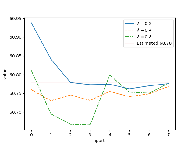
where RR is the interest rate of the riskless asset (see [2]). We take the same parameters as in [10] so T=1T=1, δ=23\delta=\frac{2}{3}, μ0=0.02\mu_{0}=0.02, σ0=0.2\sigma_{0}=0.2, vh=50v^{h}=50, vl=70v^{l}=70, γh=0.2\gamma^{h}=0.2, γl=0.02\gamma^{l}=0.02. As pointed out by [10], the solution obtained by Monte Carlo ignoring the default risk is approximately 60.7860.78. This reference can also be obtained by the algorithm taking f=0f=0 as shown on figure 4.

Refer to caption
Figure 4: Convergence of the scheme on the Black Scholes case without default taking f=0f=0 in the algorithm with a number of particle N=100000×2ipartN=100000\times 2^{\mbox{ipart}}.

Let us study the value of the different terms :

  • •

    K=(1−δ)​γh+R=0.086K=(1-\delta)\gamma^{h}+R=0.086,

  • •

    𝔼⁡(g​(XT)2)≤𝔼⁡((XT1)2)=S02​e(2​μ+σ02)​T≃10000\mathbb{E}(g(X_{T})^{2})\leq\mathbb{E}((X^{1}_{T})^{2})=S_{0}^{2}e^{(2\mu+\sigma_{0}^{2})T}\simeq 10000 where X1X^{1} stands for the first asset log value,

  • •

    Noting u^\hat{u} the solution without default

    supt∈[0,1]𝔼⁡(f​(t,Xt,u⁡(t,Xt))2)≤\displaystyle\sup_{t\in[0,1]}\mathbb{E}(f(t,X_{t},u(t,X_{t}))^{2})\leq K2​supt∈[0,1]𝔼⁡(u​(t,Xt)2)\displaystyle K^{2}\sup_{t\in[0,1]}\mathbb{E}(u(t,X_{t})^{2})
    ≤\displaystyle\leq K2​supt∈[0,1]𝔼⁡(u^​(t,Xt)2)≤K2​supt∈[0,1]𝔼⁡((Xt1)2)\displaystyle K^{2}\sup_{t\in[0,1]}\mathbb{E}(\hat{u}(t,X_{t})^{2})\leq K^{2}\sup_{t\in[0,1]}\mathbb{E}((X^{1}_{t})^{2})
    =\displaystyle= K2​S02​supt∈[0,1]e(2​μ+σ02)​t≃50.\displaystyle K^{2}S_{0}^{2}\sup_{t\in[0,1]}e^{(2\mu+\sigma_{0}^{2})t}\simeq 50.
  • •

    At last the solution may not be uniformly Lipschitz in time but remember that K^2​T2​θ\hat{K}^{2}T^{2\theta} is a bound from an expression ψ=supt∈[0,T]𝔼⁡((u^​(t,Xt)−g⁡(Xt))2)\psi=\sup_{t\in[0,T]}\mathbb{E}((\hat{u}(t,X_{t})-g(X_{t}))^{2}) so that using the previous estimations

    ψ≤2​supt∈[0,T]𝔼⁡(u​(t,Xt)2+g​(Xt)2)\displaystyle\psi\leq 2\sup_{t\in[0,T]}\mathbb{E}(u(t,X_{t})^{2}+g(X_{t})^{2})
    ≤2​S02​supt∈[0,1](e(2​μ+σ02)​t+e(2​μ+σ02)​t)≃40000\displaystyle\leq 2S_{0}^{2}\sup_{t\in[0,1]}(e^{(2\mu+\sigma_{0}^{2})t}+e^{(2\mu+\sigma_{0}^{2})t})\simeq 40000

    so that K^2​T2​θ\hat{K}^{2}T^{2\theta} can be replace 40000.40000.

In table 5, we give the coefficients of equations (33) and (34) involved in proposition 2.3.

λ\lambda 0.2 0.4 0.8
Bias p= 1 1988.0 1214.0 905.4
Bias p= 2 37.32 11.4 4.25
Bias p= 3 0.4672 0.07134 0.0133
Bias p= 4 0.004387 0.0003349 3.122e-05
Bias p= 5 3.295e-05 1.258e-06 5.863e-08
Var i = 0 28450.0 33540.0 49120.0
Var i = 1 1031.0 618.3 457.0
Var i = 2 19.13 5.77 2.139
Var i = 3 0.238 0.036 0.006682
Var i = 4 0.002226 0.0001687 1.567e-05
Table 5: Coefficient in the error analysis in proposition 2.3 for the Black Scholes case with default risk.

By taking λ=0.8\lambda=0.8 , p=3p=3, on table 6 we give the number of particles to take to have an accuracy of 0.010.01.

ii 0 1 2
NiN_{i} 110796 1030 4
Table 6: Number of particles to take for p=3,λ=0.8p=3,\lambda=0.8, an accuracy Bp+∑i=0p−1v⁡(i)Ni​∏j=0i(1+8Nj−1)=4.1​E−2.B_{p}+\sum_{i=0}^{p-1}\frac{v(i)}{N_{i}}\prod_{j=0}^{i}(1+\frac{8}{N_{j-1}})=4.1E-2.
Refer to caption
λ=0.2\lambda=0.2.
Refer to caption
λ=0.4\lambda=0.4.
Refer to caption
λ=0.8\lambda=0.8.
Figure 5: Convergence of the scheme on the Black Scholes case with default

On figure 5, we plot for different values of λ\lambda the solution obtained with one, two or three switches with a number of particles N0=36000×2 ipartN_{0}=36000\times 2^{\mbox{ ipart}}, N1=40×2 ipartN_{1}=40\times 2^{\mbox{ ipart}}, N2=2 ipartN_{2}=2^{\mbox{ ipart}}. The solution seems to be 57.2857.28 (value obtained for 33 switches with both λ=0.1\lambda=0.1 and λ=0.2\lambda=0.2 and also obtained with deep learning techniques [5]) and close to the value obtained in [10] who game 57.3057.30.
Two switches are enough to get a good accuracy. For example 57.2757.27 is reached with two switches taking N0=1152000N_{0}=1152000, N1=4480N_{1}=4480 in 9090 seconds with λ=0.2\lambda=0.2.

3 The semi linear case

In this section we extend the previous scheme obtained to the semi-linear case. To simplify the setting, without restriction, we just take a function depending on D​uDu:

(−∂tu−ℒu)(t,x)\displaystyle(-\partial_{t}u-{\cal L}u)(t,x) =f⁡(t,x,D​u​(t,x)),\displaystyle=f(t,x,Du(t,x)),
uT\displaystyle u_{T} =g,t<T,x∈ℝd,\displaystyle=g,\quad t<T,~x\in\mathbb{R}^{d}, (39)

where ℒ{\cal L} is always given by equation (2) and the dynamic of the underlying SDE is still given by (3) with μ∈ℝd\mu\in\mathbb{R}^{d}, and σ∈𝕄d\sigma\in\mathbb{M}^{d} is here some constant non-degenerated matrix.
We will take the same kind of assumption as in the previous section:

Assumption 3.1

ff is uniformly Lipschitz in D​uDu with constant KK :

|f⁡(t,x,y)−f⁡(t,x,w)|≤K​‖y−w‖2∀t∈[0,T],x∈ℝd,(w,y)∈ℝd×ℝd.\displaystyle|f(t,x,y)-f(t,x,w)|\leq K||y-w||_{2}\quad\quad\forall t\in[0,T],x\in\mathbb{R}^{d},(w,y)\in\mathbb{R}^{d}\times\mathbb{R}^{d}. (40)
Assumption 3.2

Equation (39) has a solution u∈C1,2​([0,T]×ℝd)u\in C^{1,2}([0,T]\times\mathbb{R}^{d}), such that

  • •

    D​uDu is θ\theta-Hölder with θ∈(0,1]\theta\in(0,1] in time with constant K^\hat{K} :

    ‖D​u​(t,x)−D​u​(t~,x)‖≤K^​|t−t~|θ∀(t,t~,x)∈[0,T]×[0,T]×ℝd,\displaystyle||Du(t,x)-Du(\tilde{t},x)||\leq\hat{K}|t-\tilde{t}|^{\theta}\quad\quad\quad\forall(t,\tilde{t},x)\in[0,T]\times[0,T]\times\mathbb{R}^{d},
  • •

    u⁡(t,x)u(t,x) and D​u​(t,x)Du(t,x) have a quadratic growth in xx uniformly in tt.

Assumption 3.3

gg is uniformly Lipschitz such that for K~>0\tilde{K}>0:

|g⁡(x)−g⁡(y)|≤K~​‖x−y‖2∀(x,y)∈ℝd×ℝd.\displaystyle|g(x)-g(y)|\leq\tilde{K}||x-y||_{2}\quad\forall(x,y)\in\mathbb{R}^{d}\times\mathbb{R}^{d}.

3.1 General idea of the algorithm

We will propose two algorithms that are some extensions of the algorithm previously given.
As in the previous section, the sequence (Ti)i≥0(T_{i})_{i\geq 0} is defined by equation (5) but the (τm)m≥1(\tau_{m})_{m\geq 1} are i.i.d. random variables of density ρ\rho which follow a general gamma distribution so that

ρ⁡(x)=λu​xu−1​e−λ​xΓ⁡(u),u>0\displaystyle\rho(x)=\lambda^{u}x^{u-1}\frac{e^{-\lambda x}}{\Gamma(u)},u>0 (41)

and the associated cumulated distribution function is

F⁡(x)=γ⁡(u,λ​x)Γ⁡(u),F(x)=\frac{\gamma(u,\lambda x)}{\Gamma(u)},

where γ⁡(s,x)=∫0xts−1​e−t​𝑑t\gamma(s,x)=\int_{0}^{x}t^{s-1}e^{-t}dt is the incomplete gamma function.
In order to have a converging method we will see that we will have to take u<1u<1 in ρ\rho expression (41) excluding the exponential distribution. This a weaker constraint than in [18] where, using branching for some polynomial non-linearities, converging results were only obtained for u<0.5u<0.5.

Under the regularity assumption on uu, from the Feynman-Kac formula, the representation of the solution uu is

u⁡(0,x)=\displaystyle u(0,x)= 𝔼0,x​[F¯​(T)​g⁡(WT)F¯​(T)+∫0Tf⁡(t,Xt,D​u​(t,Xt))ρ⁡(t)​ρ​(t)​𝑑t]\displaystyle\mathbb{E}_{0,x}\Big[\overline{F}(T)\frac{g(W_{T})}{\overline{F}(T)}+\int_{0}^{T}\frac{f(t,X_{t},Du(t,X_{t}))}{\rho(t)}\rho(t)dt\Big]
=\displaystyle= 𝔼0,x​[ϕ^​(0,T1,XT1,D​u​(T1,XT1))],\displaystyle\mathbb{E}_{0,x}\big[\hat{\phi}\big(0,T_{1},X_{T_{1}},Du(T_{1},X_{T_{1}})\big)\big], (42)

with

ϕ^​(s,t,x,z)\displaystyle\hat{\phi}(s,t,x,z) :=𝟏{t≥T}F¯​(T−s)​g​(x)+𝟏{t<T}ρ⁡(t−s)​f​(t,x,z).\displaystyle:=\frac{{\bf 1}_{\{t\geq T\}}}{\overline{F}(T-s)}g(x)\!+\!\frac{{\bf 1}_{\{t<T\}}}{\rho(t-s)}f(t,x,z). (43)

then we define D​u​(T1,XT1)Du(T_{1},X_{T_{1}}) using the automatic differentiation rule :

D​u​(T1,XT1)=𝔼T1,XT1​[σ−⁣⊤​WT2−WT1T2−T1​ϕ​(T1,T2,XT1,XT2,D​u​(T2,XT2))],\displaystyle Du(T_{1},X_{T_{1}})=\mathbb{E}_{T_{1},X_{T_{1}}}\Big[\sigma^{-\top}\frac{W_{T_{2}}-W_{T_{1}}}{T_{2}-T_{1}}\phi(T_{1},T_{2},X_{T_{1}},X_{T_{2}},Du(T_{2},X_{T_{2}}))\big], (44)

with

ϕ⁡(s,t,x,y,z)\displaystyle\phi(s,t,x,y,z) :=𝟏{t≥T}F¯​(T−s)​(g⁡(y)−g⁡(x))+𝟏{t<T}ρ⁡(t−s)​f​(t,y,z).\displaystyle:=\frac{{\bf 1}_{\{t\geq T\}}}{\overline{F}(T-s)}(g(y)-g(x))\!+\!\frac{{\bf 1}_{\{t<T\}}}{\rho(t-s)}f(t,y,z). (45)

where the g⁡(x)g(x) acts as a control variate term.
The automatic differentiation used here is based on the Malliavin integration by parts formula (see [14] for its use in the context of Monte Carlo approximation and the extension to other sensitivities) and has been used in a similar context as the one presented here in [8], [18].
Recursively we define for n<NTn<N_{T}:

D​un=\displaystyle Du_{n}= 𝔼Tn,XTn​[σ−⁣⊤​WTn+1−WTnTn+1−Tn​ϕ​(Tn,Tn+1,XTn,XTn+1,D​un+1)],\displaystyle\mathbb{E}_{T_{n},X_{T_{n}}}\big[\sigma^{-\top}\frac{W_{T_{n+1}}-W_{T_{n}}}{T_{n+1}-T_{n}}\phi\big(T_{n},T_{n+1},X_{T_{n}},X_{T_{n+1}},Du_{n+1}\big)\big], (46)

As in the previous section we besides consider the truncated operator after pp switches:

u0p=\displaystyle u_{0}^{p}= 𝔼⁡(ϕ^​(0,T1,XT1,D​u1p))\displaystyle\mathbb{E}\big(\hat{\phi}\big(0,T_{1},X_{T_{1}},Du_{1}^{p}\big)\big)
D​unp=\displaystyle Du_{n}^{p}= 𝔼Tn,XTnn​[σ−⁣⊤​WTn+1−WTnTn+1−Tn​ϕ​(Tn,Tn+1,XTn,XTn+1,D​un+1p)],1≤n<p\displaystyle\mathbb{E}_{T_{n},X^{n}_{T_{n}}}\big[\sigma^{-\top}\frac{W_{T_{n+1}}-W_{T_{n}}}{T_{n+1}-T_{n}}\phi\big(T_{n},T_{n+1},X_{T_{n}},X_{T_{n+1}},Du_{n+1}^{p}\big)\big],\quad 1\leq n<p
D​upp=\displaystyle Du_{p}^{p}= D​g​(XTp).\displaystyle Dg(X_{T_{p}}).

The goal of the following section is to present two algorithms based on the previously defined recursion and to show their convergence.

3.2 A first estimator

We take the same notations as in the section 2.2 for the set QiQ_{i}, i<pi<p, the set Q~​(k)\tilde{Q}(k) for k∈Qik\in Q_{i}. The τk\tau_{k} are as before some switching increments. They are always i.i.d. random variables with density ρ\rho and for k∈Qpk\in Q^{p} the W¯k\bar{W}^{k} are some independent dd-dimensional Brownian motions, independent of the (τk)k∈Qp(\tau_{k})_{k\in Q^{p}} too. The switching dates are defined by equation (5) and (Xtk~)t≥0(X^{\tilde{k}}_{t})_{t\geq 0} defined by (11).
We propose the following estimator defined by:

{u¯∅p=1N0​∑j=1N0ϕ^​(0,T(j),XT(j)(j),D​u¯(j)p),D​u¯kp=1Ni​∑k~∈Q~​(k)ϕ⁡(Tk,Tk~,XTkk,XTk~k~,D​u¯k~p)​σ−⁣⊤​W¯Tk~−Tkk~Tk~−Tk for k=(k1,k2,..ki)∈Qi,i<p,D​u¯k~p=D​g​(XTk~k~) for ​k~∈Qp\displaystyle\left\{\begin{array}[]{ll}\bar{u}_{\emptyset}^{p}=&\frac{1}{N_{0}}\sum_{j=1}^{N_{0}}\hat{\phi}\big(0,T_{(j)},X^{(j)}_{T_{(j)}},D\bar{u}_{(j)}^{p}\big),\\ D\bar{u}_{k}^{p}=&\frac{1}{N_{i}}\sum_{\tilde{k}\in\tilde{Q}(k)}\phi\big(T_{k},T_{\tilde{k}},X^{k}_{T_{k}},X^{\tilde{k}}_{T_{\tilde{k}}},D\bar{u}_{\tilde{k}}^{p}\big)\sigma^{-\top}\frac{\bar{W}_{T_{\tilde{k}}-T_{k}}^{\tilde{k}}}{T_{\tilde{k}}-T_{k}}\\ &\quad\mbox{ for }k=(k_{1},k_{2},..k_{i})\in Q_{i},i<p,\\ D\bar{u}_{\tilde{k}}^{p}=&Dg(X^{\tilde{k}}_{T_{\tilde{k}}})\quad\mbox{ for }\tilde{k}\in Q_{p}\end{array}\right.
Remark 3.4

An estimator of the gradient at the initial date is off course available too as

D​u¯∅p=\displaystyle D\bar{u}_{\emptyset}^{p}= 1N0​∑j=1N0ϕ⁡(0,T(j),x,XT(j)(j),D​u¯(j)p)​σ−⁣⊤​W¯T(j)T(j)\displaystyle\frac{1}{N_{0}}\sum_{j=1}^{N_{0}}\phi\big(0,T_{(j)},x,X^{(j)}_{T_{(j)}},D\bar{u}_{(j)}^{p}\big)\sigma^{-\top}\frac{\bar{W}_{T_{(j)}}}{T_{(j)}}
Proposition 3.5

Suppose that ρ\rho is the density of a gamma law so that ρ⁡(x)=λu​xu−1​e−λ​xΓ⁡(u)\rho(x)=\lambda^{u}x^{u-1}\frac{e^{-\lambda x}}{\Gamma(u)}, suppose that u<1u<1, and suppose that assumptions 3.1, 3.2, 3.3 are satisfied then there are two functions CC and C~\tilde{C} depending on σ\sigma and one C¯\bar{C} depending on μ\mu, σ\sigma and TT such that using estimator (3.2) to solve equation (39), we have the error estimate

𝔼⁡((u¯∅p−u⁡(0,x))2)≤∏i=1p(1+8Ni−1)​Γ​(u)p​eλ​Tλp​T(1−u)​p+1+2​θ(1−u)p−1​(2−u)​C​(σ)p−1​K^2​K2​p+\displaystyle\mathbb{E}\big((\bar{u}_{\emptyset}^{p}-u(0,x))^{2}\big)\leq\prod_{i=1}^{p}(1+\frac{8}{N_{i-1}})\frac{\Gamma(u)^{p}e^{\lambda T}}{\lambda^{p}}\frac{T^{(1-u)p+1+2\theta}}{(1-u)^{p-1}(2-u)}C(\sigma)^{p-1}\hat{K}^{2}K^{2p}+
4​∑i=0p−1K2​iNi​∏j=1i(1+8Nj−1)​Γ​(u)i+1​eλ​Tλi+1​T(1−u)​(i+1)+1(1−u)i​(2−u)​C~​(σ)i​F^+\displaystyle 4\sum_{i=0}^{p-1}\frac{K^{2i}}{N_{i}}\prod_{j=1}^{i}(1+\frac{8}{N_{j-1}})\frac{\Gamma(u)^{i+1}e^{\lambda T}}{\lambda^{i+1}}\frac{T^{(1-u)(i+1)+1}}{(1-u)^{i}(2-u)}\tilde{C}(\sigma)^{i}\hat{F}+
2​∑i=1p−1K2​iNi​∏j=1i(1+8Nj−1)​Γ​(u)i+1​eλ​Tλi​T(1−u)​i+1(1−u)i−1​(2−u)​C¯​(μ,σ,T)​C​(σ)i−1​K~2Γ⁡(u)−γ⁡(u,λ​T)+\displaystyle 2\sum_{i=1}^{p-1}\frac{K^{2i}}{N_{i}}\prod_{j=1}^{i}(1+\frac{8}{N_{j-1}})\frac{\Gamma(u)^{i+1}e^{\lambda T}}{\lambda^{i}}\frac{T^{(1-u)i+1}}{(1-u)^{i-1}(2-u)}\frac{\bar{C}(\mu,\sigma,T)C(\sigma)^{i-1}\tilde{K}^{2}}{\Gamma(u)-\gamma(u,\lambda T)}+
2N0​Γ⁡(u)Γ⁡(u)−γ⁡(u,λ​T)​𝔼​(g​(XT)2)\displaystyle\frac{2}{N_{0}}\frac{\Gamma(u)}{\Gamma(u)-\gamma(u,\lambda T)}\mathbb{E}(g(X_{T})^{2}) (51)

where

F^=supt∈[0,T]𝔼​[f​(t,Xt,D​u​(t,Xt))4]12,\displaystyle\hat{F}=\sup_{t\in[0,T]}\mathbb{E}[f(t,X_{t},Du(t,X_{t}))^{4}]^{\frac{1}{2}}, (52)

Proof. Under assumption 3.2, the solution uu of (39) satisfies a Feynman-Kac relation so that for all k~∈Q~​(∅)\tilde{k}\in\tilde{Q}(\emptyset)

u⁡(0,x)=\displaystyle u(0,x)= 𝔼0,x​[ϕ^​(0,Tk~,XTk~k~,D​u​(Tk~,XTk~k~))],\displaystyle\mathbb{E}_{0,x}\big[\hat{\phi}\big(0,T_{\tilde{k}},X_{T_{\tilde{k}}}^{\tilde{k}},Du(T_{\tilde{k}},X_{T_{\tilde{k}}}^{\tilde{k}}))\big], (53)

and that for all k∈Qik\in Q_{i} with i<pi<p, and ∀k~∈Q~​(k)\forall\tilde{k}\in\tilde{Q}(k), the gradient is given by:

D​u​(Tk,XTkk)=\displaystyle Du(T_{k},X^{k}_{T_{k}})= 𝔼Tk,XTkk​[σ−⁣⊤​W¯Tk~−Tkk~Tk~−Tk​ϕ​(Tk,Tk~,XTkk,XTk~k~,D​u​(Tk~,XTk~k~))],\displaystyle\mathbb{E}_{T_{k},X^{k}_{T_{k}}}\big[\sigma^{-\top}\frac{\bar{W}^{\tilde{k}}_{T_{\tilde{k}}-T_{k}}}{T_{\tilde{k}}-T_{k}}\phi\big(T_{k},T_{\tilde{k}},X_{T_{k}}^{k},X_{T_{\tilde{k}}}^{\tilde{k}},Du(T_{\tilde{k}},X_{T_{\tilde{k}}}^{\tilde{k}}))\big], (54)

We then introduce for k∈Qik\in Q_{i}, 1≤i<p1\leq i<p:

Ek:=\displaystyle E_{k}:= 𝔼Tk,XTkk​(‖D​u¯kp−D​u​(Tk,XTkk)‖22​1Tk<T).\displaystyle\mathbb{E}_{T_{k},X^{k}_{T_{k}}}\big(||D\bar{u}_{k}^{p}-Du(T_{k},X^{k}_{T_{k}})||^{2}_{2}1_{T_{k}<T}\big).

In exactly the same way as in the demonstration of proposition 2.3, we have the following result similar to the one given by equation (27):

Ek≤\displaystyle E_{k}\leq 1Ni​(1+8Ni)​∑k~∈Q~​(k)ETk,XTkk​((W¯τk~k~)⊤​σ−1​σ−⁣⊤​W¯τk~k~τk~2​K2ρ​(τk~)2​Ek~)+\displaystyle\frac{1}{N_{i}}(1+\frac{8}{N_{i}})\sum_{\tilde{k}\in\tilde{Q}(k)}E_{T_{k},X^{k}_{T_{k}}}\big(\frac{(\bar{W}^{\tilde{k}}_{\tau_{\tilde{k}}})^{\top}\sigma^{-1}\sigma^{-\top}\bar{W}^{\tilde{k}}_{\tau_{\tilde{k}}}}{\tau_{\tilde{k}}^{2}}\frac{K^{2}}{\rho(\tau_{\tilde{k}})^{2}}E_{\tilde{k}}\big)+
4​1Ni2​∑k~∈Q~​(k)𝔼Tk,XTkk​(1Tk~<T​(W¯τk~k~)⊤​σ−1​σ−⁣⊤​W¯τk~k~τk~2​(f⁡(Tk~,XTk~k~,D​u​(Tk~,XTk~k~))ρ⁡(τk~))2)+\displaystyle 4\frac{1}{N_{i}^{2}}\sum_{\tilde{k}\in\tilde{Q}(k)}\mathbb{E}_{T_{k},X^{k}_{T_{k}}}\big(1_{T_{\tilde{k}<T}}\frac{(\bar{W}^{\tilde{k}}_{\tau_{\tilde{k}}})^{\top}\sigma^{-1}\sigma^{-\top}\bar{W}^{\tilde{k}}_{\tau_{\tilde{k}}}}{\tau_{\tilde{k}}^{2}}(\frac{f(T_{\tilde{k}},X^{\tilde{k}}_{T_{\tilde{k}}},Du(T_{\tilde{k}},X^{\tilde{k}}_{T_{\tilde{k}}}))}{\rho(\tau_{\tilde{k}})})^{2}\big)+
2​1Ni2​∑k~∈Q~​(k)𝔼Tk,XTkk​(1Tk~≥T​(W¯T−Tkk~)⊤​σ−1​σ−⁣⊤​W¯T−Tkk~(T−Tk)2​(g⁡(XTk~)−g⁡(XTkk))2F¯​(T−Tk)2)\displaystyle 2\frac{1}{N_{i}^{2}}\sum_{\tilde{k}\in\tilde{Q}(k)}\mathbb{E}_{T_{k},X^{k}_{T_{k}}}\big(1_{T_{\tilde{k}\geq T}}\frac{(\bar{W}^{\tilde{k}}_{T-T_{k}})^{\top}\sigma^{-1}\sigma^{-\top}\bar{W}^{\tilde{k}}_{T-T_{k}}}{(T-T_{k})^{2}}\frac{(g(X^{\tilde{k}}_{T})-g(X^{k}_{T_{k}}))^{2}}{\overline{F}(T-T_{k})^{2}}\big) (55)

Using equation (27) with k=∅k=\emptyset obtained in demonstration of proposition 2.3:

𝔼⁡((u¯∅p−u⁡(0,x))2)≤\displaystyle\mathbb{E}\big((\bar{u}_{\emptyset}^{p}-u(0,x))^{2}\big)\leq 1N0​(1+8N0)​∑k~∈Q~​(∅)𝔼⁡(K2ρ​(τk~)2​Ek~)+\displaystyle\frac{1}{N_{0}}(1+\frac{8}{N_{0}})\sum_{\tilde{k}\in\tilde{Q}(\emptyset)}\mathbb{E}\big(\frac{K^{2}}{\rho(\tau_{\tilde{k}})^{2}}E_{\tilde{k}}\big)+
4​1N02​∑k~∈Q~​(∅)𝔼⁡(1Tk~<T​(f⁡(Tk~,XTk~k~,D​u​(Tk~,XTk~k~))ρ⁡(τk~))2)+\displaystyle 4\frac{1}{N_{0}^{2}}\sum_{\tilde{k}\in\tilde{Q}(\emptyset)}\mathbb{E}\big(1_{T_{\tilde{k}<T}}(\frac{f(T_{\tilde{k}},X^{\tilde{k}}_{T_{\tilde{k}}},Du(T_{\tilde{k}},X^{\tilde{k}}_{T_{\tilde{k}}}))}{\rho(\tau_{\tilde{k}})})^{2}\big)+
2​1N02​∑k~∈Q~​(∅)𝔼Tk,XTkk​(1Tk~≥T​g​(XTk~)2F¯​(T−Tk)2).\displaystyle 2\frac{1}{N_{0}^{2}}\sum_{\tilde{k}\in\tilde{Q}(\emptyset)}\mathbb{E}_{T_{k},X^{k}_{T_{k}}}\big(1_{T_{\tilde{k}\geq T}}\frac{g(X^{\tilde{k}}_{T})^{2}}{\overline{F}(T-T_{k})^{2}}\big). (56)

Iterating from 1 to p−1p-1 we get:

𝔼⁡((u¯∅p−u⁡(0,x))2)≤\displaystyle\mathbb{E}\big((\bar{u}_{\emptyset}^{p}-u(0,x))^{2}\big)\leq A1+4​A2+2​A3,\displaystyle A_{1}+4A_{2}+2A_{3}, (57)

where

A1=∏i=1p1Ni−1(1+8Ni−1)∑k~1∈Q~​(∅)…∑k~p∈Q~​(k~p−1)B1(k~1,..,k~P)\displaystyle A_{1}=\prod_{i=1}^{p}\frac{1}{N_{i-1}}(1+\frac{8}{N_{i-1}})\sum_{\tilde{k}^{1}\in\tilde{Q}(\emptyset)}...\sum_{\tilde{k}^{p}\in\tilde{Q}(\tilde{k}^{p-1})}B_{1}(\tilde{k}^{1},..,\tilde{k}^{P}) (58)
A2=∑i=0p−1K2​iNi2∏j=1i1Nj−1(1+8Nj−1),∑k~1∈Q~​(∅)…∑k~i+1∈Q~​(k~i)B2(k~1,..,k~i+1),\displaystyle A_{2}=\sum_{i=0}^{p-1}\frac{K^{2i}}{N_{i}^{2}}\prod_{j=1}^{i}\frac{1}{N_{j-1}}(1+\frac{8}{N_{j-1}}),\sum_{\tilde{k}^{1}\in\tilde{Q}(\emptyset)}...\sum_{\tilde{k}^{i+1}\in\tilde{Q}(\tilde{k}^{i})}B_{2}(\tilde{k}^{1},..,\tilde{k}^{i+1}), (59)

and

A3=∑i=0p−1K2​iNi2∏j=1i1Nj−1(1+8Nj−1)∑k~1∈Q~​(∅)…∑k~i+1∈Q~​(k~i)B3(k~1,..,k~i+1),\displaystyle A_{3}=\sum_{i=0}^{p-1}\frac{K^{2i}}{N_{i}^{2}}\prod_{j=1}^{i}\frac{1}{N_{j-1}}(1+\frac{8}{N_{j-1}})\sum_{\tilde{k}^{1}\in\tilde{Q}(\emptyset)}...\sum_{\tilde{k}^{i+1}\in\tilde{Q}(\tilde{k}^{i})}B_{3}(\tilde{k}^{1},..,\tilde{k}^{i+1}), (60)

where noting

ψk=(W¯τkk)⊤​σ−1​σ−⁣⊤​W¯τkkτk2,\displaystyle\psi_{k}=\frac{(\bar{W}^{k}_{\tau_{k}})^{\top}\sigma^{-1}\sigma^{-\top}\bar{W}^{k}_{\tau_{k}}}{\tau_{k}^{2}},
f^k=f⁡(Tk,XTkk,D​u​(Tk,XTkk)),\displaystyle\hat{f}_{k}=f(T_{k},X^{k}_{T_{k}},Du(T_{k},X^{k}_{T_{k}})), (61)

we have:

B1(k~1,..,k~P)=\displaystyle B_{1}(\tilde{k}^{1},..,\tilde{k}^{P})= 𝔼⁡[∏j=1pK2ρ​(τk~j)2​∏j=2pψk~j​Ek~p],\displaystyle\mathbb{E}[\prod_{j=1}^{p}\frac{K^{2}}{\rho(\tau_{\tilde{k}^{j}})^{2}}\prod_{j=2}^{p}\psi_{\tilde{k}^{j}}E_{\tilde{k}^{p}}],
B2(k~1,..,k~i+1)=\displaystyle B_{2}(\tilde{k}^{1},..,\tilde{k}^{i+1})= 𝔼⁡[1Tk~i+1<T​(f^k~i+1)2​∏j=1i+11ρ​(τk~j)2​∏j=2i+1ψk~j],\displaystyle\mathbb{E}\big[1_{T_{\tilde{k}^{i+1}<T}}(\hat{f}_{\tilde{k}^{i+1}})^{2}\prod_{j=1}^{i+1}\frac{1}{\rho(\tau_{\tilde{k}^{j}})^{2}}\prod_{j=2}^{i+1}\psi_{\tilde{k}^{j}}\Big],
B3(k~1,..,k~i+1)=\displaystyle B_{3}(\tilde{k}^{1},..,\tilde{k}^{i+1})= 𝔼[1Tk~i+1≥T1Tk~i<T(g⁡(XTk~i+1)−1i≥1​g​(XTk~ik~i))2F¯​(T−Tk~i)2∏j=1i1ρ​(τk~j)2∏j=2iψk~j\displaystyle\mathbb{E}\big[1_{T_{\tilde{k}^{i+1}\geq T}}1_{T_{\tilde{k}^{i}<T}}\frac{(g(X^{\tilde{k}^{i+1}}_{T})-1_{i\geq 1}g(X^{\tilde{k}^{i}}_{T_{\tilde{k}^{i}}}))^{2}}{\bar{F}(T-T_{\tilde{k}^{i}})^{2}}\prod_{j=1}^{i}\frac{1}{\rho(\tau_{\tilde{k}^{j}})^{2}}\prod_{j=2}^{i}\psi_{\tilde{k}^{j}}
(W¯T−Tk~ik~i+1)⊤​σ−1​σ−⁣⊤​W¯T−Tk~ik~i+1(T−Tk~i)2],\displaystyle\frac{(\bar{W}^{\tilde{k}^{i+1}}_{T-T_{\tilde{k}^{i}}})^{\top}\sigma^{-1}\sigma^{-\top}\bar{W}^{\tilde{k}^{i+1}}_{T-T_{\tilde{k}^{i}}}}{(T-T_{\tilde{k}^{i}})^{2}}\big], (62)

where Ek~p=1Tk~p<T​(D​g​(XTk~pk~p)−D​u​(Tk~p,XTk~pk~p))2E_{\tilde{k}^{p}}=1_{T_{\tilde{k}^{p}<T}}(Dg(X_{T_{\tilde{k}^{p}}}^{\tilde{k}^{p}})-Du(T_{\tilde{k}^{p}},X_{T_{\tilde{k}^{p}}}^{\tilde{k}^{p}}))^{2}.
We first bound B1B_{1}.
We introduce ψk=ϕkτk\psi_{k}=\frac{\phi_{k}}{\tau_{k}}, where

ϕk=Gk⊤​σ−1​σ−⁣⊤​Gk,\displaystyle\phi_{k}=G_{k}^{\top}\sigma^{-1}\sigma^{-\top}G_{k}, (63)

and Gk∈ℝdG_{k}\in\mathbb{R}^{d} is composed of centered unitary independent Gaussian random variables.
We introduce C⁡(σ)=𝔼⁡(ϕk)C(\sigma)=\mathbb{E}(\phi_{k}) which is independent of kk. Using the Hölder property of D​uDu, the tower property, the independence of the τk\tau_{k} an the ϕk\phi_{k}, we get:

B1(k~1,..,k~P)=\displaystyle B_{1}(\tilde{k}^{1},..,\tilde{k}^{P})= 𝔼[∏j=1pK2ρ​(τk~j)2(∏j=2p1τk~j)𝔼(Ek~p∏j=2pϕk~j|τk~1,..,τk~p)]\displaystyle\mathbb{E}[\prod_{j=1}^{p}\frac{K^{2}}{\rho(\tau_{\tilde{k}^{j}})^{2}}(\prod_{j=2}^{p}\frac{1}{\tau_{\tilde{k}^{j}}})\mathbb{E}(E_{\tilde{k}^{p}}\prod_{j=2}^{p}\phi_{\tilde{k}^{j}}|\tau_{\tilde{k}^{1}},..,\tau_{\tilde{k}^{p}})]
≤\displaystyle\leq K^2​T2​θ​K2​p​C​(σ)p−1​E​[1Tk~p<T​∏j=1p1ρ​(τk~j)2​∏j=2p1τk~j].\displaystyle\hat{K}^{2}T^{2\theta}K^{2p}C(\sigma)^{p-1}E[1_{T_{\tilde{k}^{p}<T}}\prod_{j=1}^{p}\frac{1}{\rho(\tau_{\tilde{k}^{j}})^{2}}\prod_{j=2}^{p}\frac{1}{\tau_{\tilde{k}^{j}}}].

Using the expression for the density of ρ\rho given by (41), we have the bound:

H:=\displaystyle H:= E⁡[1Tk~p<T​∏j=1p1ρ​(τk~j)2​∏j=2p1τk~j]\displaystyle E[1_{T_{\tilde{k}^{p}<T}}\prod_{j=1}^{p}\frac{1}{\rho(\tau_{\tilde{k}^{j}})^{2}}\prod_{j=2}^{p}\frac{1}{\tau_{\tilde{k}^{j}}}]
≤\displaystyle\leq Γ​(u)p​eλ​Tλp​∫0T1xu−1​𝑑x(∫0T1xu​𝑑x)p−1\displaystyle\frac{\Gamma(u)^{p}e^{\lambda T}}{\lambda^{p}}\int_{0}^{T}\frac{1}{x^{u-1}}dx\quad(\int_{0}^{T}\frac{1}{x^{u}}dx)^{p-1}
=\displaystyle= Γ​(u)p​eλ​Tλp​T(1−u)​p+1(1−u)p−1​(2−u),\displaystyle\frac{\Gamma(u)^{p}e^{\lambda T}}{\lambda^{p}}\frac{T^{(1-u)p+1}}{(1-u)^{p-1}(2-u)}, (64)

so that

B1(k~1,..,k~P)≤Γ​(u)p​eλ​TλpT(1−u)​p+1+2​θ(1−u)p−1​(2−u)C(σ)p−1K^2K2​p.\displaystyle B_{1}(\tilde{k}^{1},..,\tilde{k}^{P})\leq\frac{\Gamma(u)^{p}e^{\lambda T}}{\lambda^{p}}\frac{T^{(1-u)p+1+2\theta}}{(1-u)^{p-1}(2-u)}C(\sigma)^{p-1}\hat{K}^{2}K^{2p}. (65)

In a similar way introducing C~​(σ)=𝔼​(ϕk2)12\tilde{C}(\sigma)=\mathbb{E}(\phi_{k}^{2})^{\frac{1}{2}} and using the tower rule, the independence of the different random variables and Cauchy Schwartz,

B2(k~1,..,k~i+1)\displaystyle B_{2}(\tilde{k}^{1},..,\tilde{k}^{i+1}) =𝔼(1Tk~i+1<T𝔼(f^k~i+12∏j=2i+1ϕk~j/τk~1,..,τk~i+1)1ρ​(τk~1)2∏j=2i+11ρ​(τk~j)2​τk~j)\displaystyle=\mathbb{E}\big(1_{T_{\tilde{k}^{i+1}}<T}\mathbb{E}(\hat{f}_{\tilde{k}^{i+1}}^{2}\prod_{j=2}^{i+1}\phi_{\tilde{k}^{j}}/\tau_{\tilde{k}^{1}},..,\tau_{\tilde{k}^{i+1}})\frac{1}{\rho(\tau_{\tilde{k}^{1}})^{2}}\prod_{j=2}^{i+1}\frac{1}{\rho(\tau_{\tilde{k}^{j}})^{2}\tau_{\tilde{k}^{j}}}\big)
≤supt∈[0,T]𝔼​[f​(t,Xt,D​u​(t,Xt))4]12​𝔼​(∏j=2i+1ϕk~j2)12​E​(1Tk~i+1<T​1ρ​(τk~1)2​∏j=2i+11ρ​(τk~j)2​τk~j)\displaystyle\leq\sup_{t\in[0,T]}\mathbb{E}[f(t,X_{t},Du(t,X_{t}))^{4}]^{\frac{1}{2}}\mathbb{E}(\prod_{j=2}^{i+1}\phi_{\tilde{k}^{j}}^{2})^{\frac{1}{2}}E\big(1_{T_{\tilde{k}^{i+1}}<T}\frac{1}{\rho(\tau_{\tilde{k}^{1}})^{2}}\prod_{j=2}^{i+1}\frac{1}{\rho(\tau_{\tilde{k}^{j}})^{2}\tau_{\tilde{k}^{j}}}\big)
≤Γ​(u)i+1​eλ​Tλi+1​T(1−u)​(i+1)+1(1−u)i​(2−u)​C~​(σ)i​supt∈[0,T]𝔼​[f​(t,Xt,D​u​(t,Xt))4]12.\displaystyle\leq\frac{\Gamma(u)^{i+1}e^{\lambda T}}{\lambda^{i+1}}\frac{T^{(1-u)(i+1)+1}}{(1-u)^{i}(2-u)}\tilde{C}(\sigma)^{i}\sup_{t\in[0,T]}\mathbb{E}[f(t,X_{t},Du(t,X_{t}))^{4}]^{\frac{1}{2}}. (66)

For B3B_{3} we divide the calculation into two cases :

B3​(k~1)=\displaystyle B_{3}(\tilde{k}^{1})= 𝔼⁡(1τk~1>T​1F¯​(T)2​𝔼​(g​(XT)2))\displaystyle\mathbb{E}(1_{\tau_{\tilde{k}^{1}}>T}\frac{1}{\bar{F}(T)^{2}}\mathbb{E}(g(X_{T})^{2}))
=\displaystyle= 1F¯​(T)​𝔼​(g​(XT)2)\displaystyle\frac{1}{\bar{F}(T)}\mathbb{E}(g(X_{T})^{2})
=\displaystyle= Γ⁡(u)Γ⁡(u)−γ⁡(u,λ​T)​𝔼​(g​(XT)2).\displaystyle\frac{\Gamma(u)}{\Gamma(u)-\gamma(u,\lambda T)}\mathbb{E}(g(X_{T})^{2}). (67)

For i>0i>0, using the Lipschitz property of gg, the tower property, the independence of the different random variables, and noting

C¯​(μ,σ,T)=𝔼⁡[(2​‖μ‖22​T+2​‖σ​Gk~i+1‖22)​ϕk~i+1],\bar{C}(\mu,\sigma,T)=\mathbb{E}[(2||\mu||_{2}^{2}T+2||\sigma G_{\tilde{k}^{i+1}}||_{2}^{2})\phi_{\tilde{k}^{i+1}}],

we have the following bound:

B3​(k~1,…,k~i+1)≤\displaystyle B_{3}(\tilde{k}^{1},...,\tilde{k}^{i+1})\leq 𝔼⁡[1Tk~i+1>T​1Tk~i<T​K~2​(2​‖μ‖22​T+2​‖σ​Gk~i+1‖22)​ϕk~i+1F¯​(T)2​C​(σ)i−1ρ​(τk~1)2​∏j=2i1ρ​(τk~j)2​τk~j]\displaystyle\mathbb{E}\big[1_{T_{\tilde{k}^{i+1}>T}}1_{T_{\tilde{k}^{i}<T}}\tilde{K}^{2}\frac{(2||\mu||_{2}^{2}T+2||\sigma G_{\tilde{k}^{i+1}}||_{2}^{2})\phi_{\tilde{k}^{i+1}}}{\bar{F}(T)^{2}}\frac{C(\sigma)^{i-1}}{\rho(\tau_{\tilde{k}^{1}})^{2}}\prod_{j=2}^{i}\frac{1}{\rho(\tau_{\tilde{k}^{j}})^{2}\tau_{\tilde{k}^{j}}}\big]
≤\displaystyle\leq C¯​(μ,σ,T)​K~2F¯​(T)2​C​(σ)i−1​Γ​(u)i​eλ​Tλi​∫0T1xu−1​𝑑x(∫0T1xu​𝑑x)i−1​∫T∞ρ⁡(x)​𝑑x\displaystyle\frac{\bar{C}(\mu,\sigma,T)\tilde{K}^{2}}{\bar{F}(T)^{2}}C(\sigma)^{i-1}\frac{\Gamma(u)^{i}e^{\lambda T}}{\lambda^{i}}\int_{0}^{T}\frac{1}{x^{u-1}}dx\quad(\int_{0}^{T}\frac{1}{x^{u}}dx)^{i-1}\int_{T}^{\infty}\rho(x)dx
=\displaystyle= C​(σ)i−1​Γ​(u)i+1λi​T(1−u)​i+1(1−u)i−1​(2−u)​C¯​(μ,σ,T)​K~2​eλ​TΓ⁡(u)−γ⁡(u,λ​T).\displaystyle C(\sigma)^{i-1}\frac{\Gamma(u)^{i+1}}{\lambda^{i}}\frac{T^{(1-u)i+1}}{(1-u)^{i-1}(2-u)}\frac{\bar{C}(\mu,\sigma,T)\tilde{K}^{2}e^{\lambda T}}{\Gamma(u)-\gamma(u,\lambda T)}. (68)

Plugging (65), (66), (67), (68) into (58), (59) and (60) that we insert into (57) gives the desired estimation.

3.3 A second estimator

In this section we present a scheme derived from [26].
We extend the notations from the previous section 3.2. Let set p∈ℕ∗p\in\mathbb{N}^{*}. We construct the sets QioQ^{o}_{i} for i=1,..,pi=1,..,p, such that Q1o={(k1),(k1−)}Q^{o}_{1}=\{(k_{1}),(k_{1}^{-})\} where k1∈{1,..,N1}k_{1}\in\{1,..,N_{1}\}, so that to a particle noted (k1)∈Q1(k_{1})\in Q_{1}, we associate a antithetic particle noted k1−k_{1}^{-}. Then the set QioQ^{o}_{i} are defined by recurrence :

Qi+1o={(k1,..,ki,ki+1)/(k1,..,ki)∈Qio,ki+1∈{1,..,Ni+1,1−,..,Ni+1−}}\displaystyle Q^{o}_{i+1}=\{(k_{1},..,k_{i},k_{i+1})/(k_{1},..,k_{i})\in Q^{o}_{i},k_{i+1}\in\{1,..,N_{i+1},1^{-},..,N^{-}_{i+1}\}\}

To a particle k=(k1,..,ki)∈Qiok=(k_{1},..,k_{i})\in Q^{o}_{i} we associate its original particle o⁡(k)∈Qio(k)\in Q_{i} such that o(k)=(k^1,..k^i)o(k)=(\hat{k}_{1},..\hat{k}_{i}) where k^j=l\hat{k}_{j}=l if kj=lk_{j}=l or l−l^{-}. Further, when k=(k1,⋯,ki)k=(k_{1},\cdots,k_{i}) is such that ki∈ℕk_{i}\in\mathbb{N}, we denote k−:=(k1,⋯,ki−1,ki−)k^{-}:=(k_{1},\cdots,k_{i-1},k_{i}^{-}).
By convention Tk=To⁡(k)T_{k}=T_{o(k)}, τk=τo⁡(k)\tau_{k}=\tau_{o(k)} and W¯tk=W¯to⁡(k)\bar{W}_{t}^{k}=\bar{W}_{t}^{o(k)}. For k=(k1,…,ki)∈Qiok=(k_{1},...,k_{i})\in Q^{o}_{i} we introduce the set

  • •

    Q~o(k)={l=(k1,..,ki,m)/m∈{1,..,Ni}}⊂Qi+1o\tilde{Q}^{o}(k)=\{l=(k_{1},..,k_{i},m)/m\in\{1,..,N_{i}\}\}\subset Q_{i+1}^{o}

  • •

    and Q^o(k)={l=(k1,..,ki,m)/m∈{1,..,Ni,1−,..,Ni−}}⊂Qi+1o\hat{Q}^{o}(k)=\{l=(k_{1},..,k_{i},m)/m\in\{1,..,N_{i},1^{-},..,N_{i}^{-}\}\}\subset Q_{i+1}^{o}

For k=(k1,..,ki)∈Qiok=(k_{1},..,k_{i})\in Q^{o}_{i} and k~=(k1,..,ki,ki+1)∈Q^o(k)\tilde{k}=(k_{1},..,k_{i},k_{i+1})\in\hat{Q}^{o}(k) we define the following trajectories :

Wsk~:=\displaystyle W^{\tilde{k}}_{s}~:=~ WTkk+𝟏ki+1∈ℕ​W¯s−Tko⁡(k~)−𝟏ki+1∉ℕ​W¯s−Tko⁡(k~),and\displaystyle W^{k}_{T_{k}}~+~{\bf 1}_{k_{i+1}\in\mathbb{N}}\bar{W}^{o(\tilde{k})}_{s-T_{k}}~-~{\bf 1}_{k_{i+1}\notin\mathbb{N}}\bar{W}^{o(\tilde{k})}_{s-T_{k}},~~~\mbox{and}~~ (69)
Xsk~:=\displaystyle X^{\tilde{k}}_{s}:= x+μ​s+σ​Wsk~,∀s∈[Tk,Tk~].\displaystyle x+\mu s+\sigma W^{\tilde{k}}_{s},~~~\forall s\in[T_{k},T_{\tilde{k}}]. (70)

Using the previous definitions, we consider the estimator defined by:

{u¯0p=OPEN1N0​∑j=1N0(ϕ^​(0,T(j),XT(j)(j),D​u¯(j)p)+ϕ^​(0,T(j),XT(j)(j)−,D​u¯(j)−p))2),D​u¯kp=1Ni​∑k~∈Q~o​(k)W~k~​12​(ϕ^​(Tk,Tk~,XTk~k~,D​u¯k~p)−ϕ^​(Tk,Tk~,XTk~k~−,D​u¯k~−p)), for k=(k1,..ki)∈Qoi,i<p,D​u¯k~p=D​g​(XTk~k~)for ​k~∈Qpo\displaystyle\left\{\begin{array}[]{ll}\bar{u}_{0}^{p}=&\frac{1}{N_{0}}\sum_{j=1}^{N_{0}}\frac{\big(\hat{\phi}\big(0,T_{(j)},X^{(j)}_{T_{(j)}},D\bar{u}_{(j)}^{p}\big)+\hat{\phi}\big(0,T_{(j)},X^{(j)^{-}}_{T_{(j)}},D\bar{u}_{(j)^{-}}^{p}\big)\big)}{2}\big),\\ D\bar{u}_{k}^{p}=&\frac{1}{N_{i}}\sum_{\tilde{k}\in\tilde{Q}^{o}(k)}\tilde{W}^{\tilde{k}}\frac{1}{2}\big(\hat{\phi}\big(T_{k},T_{\tilde{k}},X^{\tilde{k}}_{T_{\tilde{k}}},D\bar{u}_{\tilde{k}}^{p}\big)-\hat{\phi}\big(T_{k},T_{\tilde{k}},X^{\tilde{k}^{-}}_{T_{\tilde{k}}},D\bar{u}_{\tilde{k}^{-}}^{p}\big)\big),\\ &\quad\mbox{ for }k=(k_{1},..k_{i})\in Q^{o}_{i},i<p,\\ D\bar{u}_{\tilde{k}}^{p}=&Dg(X^{\tilde{k}}_{T_{\tilde{k}}})\quad\mbox{for }\tilde{k}\in Q_{p}^{o}\end{array}\right.

where ϕ^\hat{\phi} is defined by equation (43) and W~k~=σ−⁣⊤​W¯Tk~−Tko⁡(k~)Tk~−Tk\tilde{W}^{\tilde{k}}=\sigma^{-\top}\frac{\bar{W}_{T_{\tilde{k}}-T_{k}}^{o(\tilde{k})}}{T_{\tilde{k}}-T_{k}} .
The idea is that, for a given k=(k1,..,ki)∈Qiok=(k_{1},..,k_{i})\in Q^{o}_{i} and a given k~∈Q~o​(k)\tilde{k}\in\tilde{Q}^{o}(k), if we have W¯Tk~−Tk\bar{W}_{T_{\tilde{k}}-T_{k}} very small then

12​(ϕ^​(Tk,Tk~,XTk~k~,D​u¯k~p)−ϕ^​(Tk,Tk~,XTk~k~−,D​u¯k~−p))≃\displaystyle\frac{1}{2}\big(\hat{\phi}\big(T_{k},T_{\tilde{k}},X^{\tilde{k}}_{T_{\tilde{k}}},D\bar{u}_{\tilde{k}}^{p}\big)-\hat{\phi}\big(T_{k},T_{\tilde{k}},X^{\tilde{k}^{-}}_{T_{\tilde{k}}},D\bar{u}_{\tilde{k}^{-}}^{p})\big)\simeq Du​ϕ^​(Tk,Tk~,XTk~k~,D​u¯k~p)​(D​u¯k~p−D​u¯k~−p)+\displaystyle D_{u}\hat{\phi}\big(T_{k},T_{\tilde{k}},X^{\tilde{k}}_{T_{\tilde{k}}},D\bar{u}_{\tilde{k}}^{p}\big)(D\bar{u}_{\tilde{k}}^{p}-D\bar{u}_{\tilde{k}^{-}}^{p}\big)+
Dx​ϕ^​(Tk,Tk~,XTk~k~,D​u¯k~p)​(XTk~k~−XTk~k~−)\displaystyle D_{x}\hat{\phi}\big(T_{k},T_{\tilde{k}},X^{\tilde{k}}_{T_{\tilde{k}}},D\bar{u}_{\tilde{k}}^{p}\big)(X^{\tilde{k}}_{T_{\tilde{k}}}-X^{\tilde{k}^{-}}_{T_{\tilde{k}}})
≃\displaystyle\simeq C​τk~.\displaystyle C\sqrt{\tau^{\tilde{k}}}.

So W~k~​12​(ϕ^​(Tk,Tk~,XTk~k~,D​u¯k~p)−ϕ^​(Tk,Tk~,XTk~k~−,D​u¯k~−p))\tilde{W}^{\tilde{k}}\frac{1}{2}\big(\hat{\phi}\big(T_{k},T_{\tilde{k}},X^{\tilde{k}}_{T_{\tilde{k}}},D\bar{u}_{\tilde{k}}^{p}\big)-\hat{\phi}\big(T_{k},T_{\tilde{k}},X^{\tilde{k}^{-}}_{T_{\tilde{k}}},D\bar{u}_{\tilde{k}^{-}}^{p})\big), as function of τk~\tau^{\tilde{k}}, should be bounded, and we hope that estimator (3.3) has a much smaller variance than estimator (3.2).

Remark 3.6

As in a previous scheme an estimation of the gradient is obtained as:

D​u¯0p=\displaystyle D\bar{u}_{0}^{p}= 1N0​∑j=1N012​σ−⁣⊤​WT(j)T(j)​(ϕ^​(0,T(j),XT(j)(j),D​u¯(j)p)−ϕ^​(0,T(j),XT(j)(j)−,D​u¯(j)−p))\displaystyle\frac{1}{N_{0}}\sum_{j=1}^{N_{0}}\frac{1}{2}\sigma^{-\top}\frac{W_{T_{(j)}}}{T_{(j)}}\big(\hat{\phi}\big(0,T_{(j)},X^{(j)}_{T_{(j)}},D\bar{u}_{(j)}^{p}\big)-\hat{\phi}\big(0,T_{(j)},X^{(j)^{-}}_{T_{(j)}},D\bar{u}_{(j)^{-}}^{p}\big)\big)

We need other assumptions on the solution and the driver to fully exploit this scheme:

Assumption 3.7

D​uDu is uniformly Lipschitz in xx such that for K¯>0\bar{K}>0:

‖D​u​(t,x)−D​u​(t,y)‖2≤K¯​‖x−y‖2∀(t,x,y)∈[0,T]×ℝd×ℝd.\displaystyle||Du(t,x)-Du(t,y)||_{2}\leq\bar{K}||x-y||_{2}\quad\forall(t,x,y)\in[0,T]\times\mathbb{R}^{d}\times\mathbb{R}^{d}.
Assumption 3.8

ff is uniformly Lipschitz in xx such that there exists K¯>0\underline{K}>0

|f⁡(t,x,z)−f⁡(t,y,z)|≤K¯​‖x−y‖2,∀(t,x,y,z)∈[0,T]×ℝd×ℝd×ℝd.\displaystyle|f(t,x,z)-f(t,y,z)|\leq\underline{K}||x-y||_{2},\quad\forall(t,x,y,z)\in[0,T]\times\mathbb{R}^{d}\times\mathbb{R}^{d}\times\mathbb{R}^{d}.

We now give the error estimate with the second scheme

Proposition 3.9

Suppose that ρ\rho is the density of a gamma law so that ρ⁡(x)=λu​xu−1​e−λ​xΓ⁡(u)\rho(x)=\lambda^{u}x^{u-1}\frac{e^{-\lambda x}}{\Gamma(u)}, suppose that u<1u<1, and suppose that assumptions 3.1, 3.2, 3.3,3.7 and 3.8 are satisfied then there are two functions CC and C~\tilde{C} depending on σ\sigma and one C¯\bar{C} depending on KK, K¯\bar{K}, K¯\underline{K} and σ\sigma such that using estimator (3.3) to solve equation (39), we have the error estimate

𝔼⁡((u¯∅p−u⁡(0,x))2)≤∏i=1p(1+8Ni−1)​Γ​(u)p​eλ​Tλp​T(1−u)​p+1+2​θ(1−u)p−1​(2−u)​C​(σ)p−1​K^2​K2​p+\displaystyle\mathbb{E}\big((\bar{u}_{\emptyset}^{p}-u(0,x))^{2}\big)\leq\prod_{i=1}^{p}(1+\frac{8}{N_{i-1}})\frac{\Gamma(u)^{p}e^{\lambda T}}{\lambda^{p}}\frac{T^{(1-u)p+1+2\theta}}{(1-u)^{p-1}(2-u)}C(\sigma)^{p-1}\hat{K}^{2}K^{2p}+
∑i=1p−1K2​iNi​∏j=1i(1+8Nj−1)​C¯​(σ,K,K¯,K¯)​C​(σ)i−1​Γ​(u)i+1​eλ​Tλi+1​T(1−u)​i+3−u(2−u)2​(1−u)i−1+\displaystyle\sum_{i=1}^{p-1}\frac{K^{2i}}{N_{i}}\prod_{j=1}^{i}(1+\frac{8}{N_{j-1}})\bar{C}(\sigma,K,\bar{K},\underline{K})C(\sigma)^{i-1}\frac{\Gamma(u)^{i+1}e^{\lambda T}}{\lambda^{i+1}}\frac{T^{(1-u)i+3-u}}{(2-u)^{2}(1-u)^{i-1}}+
∑i=1p−1K2​i2​Ni​∏j=1i(1+8Nj−1)​C​(σ)i−1​K~2​Γ​(u)i+1​eλ​Tλi​(Γ⁡(u)−γ⁡(u,λ​T))​C¯​(σ)​T(1−u)​i+1(2−u)​(1−u)i−1+\displaystyle\sum_{i=1}^{p-1}\frac{K^{2i}}{2N_{i}}\prod_{j=1}^{i}(1+\frac{8}{N_{j-1}})C(\sigma)^{i-1}\frac{\tilde{K}^{2}\Gamma(u)^{i+1}e^{\lambda T}}{\lambda^{i}(\Gamma(u)-\gamma(u,\lambda T))}\bar{C}(\sigma)\frac{T^{(1-u)i+1}}{(2-u)(1-u)^{i-1}}+
4N0​Γ⁡(u)λ​eλ​T​T2−u2−u​F^+2N0​Γ⁡(u)Γ⁡(u)−γ⁡(u,λ​T)​𝔼​(g​(XT)2)\displaystyle\frac{4}{N_{0}}\frac{\Gamma(u)}{\lambda}e^{\lambda T}\frac{T^{2-u}}{2-u}\hat{F}+\frac{2}{N_{0}}\frac{\Gamma(u)}{\Gamma(u)-\gamma(u,\lambda T)}\mathbb{E}(g(X_{T})^{2}) (75)

with F^\hat{F} given by equation (52).

Proof. First notice that under assumption 3.2, uu satisfies (42) and then, for j∈[0,N0]j\in[0,N_{0}]

u⁡(0,x)=𝔼0,x​[ϕ^​(0,T(j),XT(j)(j),D​u​(T(j),XT(j)(j)))+ϕ^​(0,T(j),XT(j)(j)−,D​u​(T(j),XT(j)(j)−)CLOSE2],\displaystyle u(0,x)=\mathbb{E}_{0,x}\big[\frac{\hat{\phi}\big(0,T_{(j)},X^{(j)}_{T_{(j)}},Du(T_{(j)},X^{(j)}_{T_{(j)}})\big)+\hat{\phi}\big(0,T_{(j)},X^{(j)^{-}}_{T_{(j)}},Du(T_{(j)},X^{(j)^{-}}_{T_{(j)}}\big)}{2}\big],

and because uu satisfies equation (44), we have that for k∈Qiok\in Q^{o}_{i}, k~∈Q~o​(k)\tilde{k}\in\tilde{Q}^{o}(k),

D​u​(Tk,Xtkk)=\displaystyle Du(T_{k},X^{k}_{t_{k}})= 𝔼Tk,Xtkk​(σ−⁣⊤​W¯Tk~−Tko⁡(k~)Tk~−Tk​12​(ϕ^​(Tk,Tk~,XTk~k~,D​u​(Tk~,XTk~k~))−ϕ^​(Tk,Tk~,XTk~k~−,D​u​(Tk~,XTk~k~−)))CLOSE\displaystyle\mathbb{E}_{T_{k},X^{k}_{t_{k}}}\big(\sigma^{-\top}\frac{\bar{W}_{T_{\tilde{k}}-T_{k}}^{o(\tilde{k})}}{T_{\tilde{k}}-T_{k}}\frac{1}{2}\big(\hat{\phi}\big(T_{k},T_{\tilde{k}},X^{\tilde{k}}_{T_{\tilde{k}}},Du(T_{\tilde{k}},X^{\tilde{k}}_{T_{\tilde{k}}})\big)-\hat{\phi}\big(T_{k},T_{\tilde{k}},X^{\tilde{k}^{-}}_{T_{\tilde{k}}},Du(T_{\tilde{k}},X^{\tilde{k}^{-}}_{T_{\tilde{k}}})\big)\big)

Then we can introduce for k∈Qik\in Q_{i}, 1≤i<p1\leq i<p:

Ek:=\displaystyle E_{k}:= 𝔼Tk,XTkk​(‖D​u¯kp−D​u​(Tk,XTkk)‖22​1Tk<T).\displaystyle\mathbb{E}_{T_{k},X^{k}_{T_{k}}}\big(||D\bar{u}_{k}^{p}-Du(T_{k},X^{k}_{T_{k}})||^{2}_{2}1_{T_{k}<T}\big).

In exactly the same way as in the demonstration of proposition 3.5, we have the following result similar to the one given by equation (55):

Ek≤\displaystyle E_{k}\leq 1Ni​(1+8Ni)​∑k~∈Q~o​(k)ETk,XTkk​(1Tk~<T​(W¯τk~k~)⊤​σ−1​σ−⁣⊤​W¯τk~k~τk~2​14​ρ​(τk~)2​(f⁡(Tk~,XTk~k~,D​u¯k~p)−CLOSECLOSE\displaystyle\frac{1}{N_{i}}(1+\frac{8}{N_{i}})\sum_{\tilde{k}\in\tilde{Q}^{o}(k)}E_{T_{k},X^{k}_{T_{k}}}\big(1_{T_{\tilde{k}<T}}\frac{(\bar{W}^{\tilde{k}}_{\tau_{\tilde{k}}})^{\top}\sigma^{-1}\sigma^{-\top}\bar{W}^{\tilde{k}}_{\tau_{\tilde{k}}}}{\tau_{\tilde{k}}^{2}}\frac{1}{4\rho(\tau_{\tilde{k}})^{2}}\big(f(T_{\tilde{k}},X^{\tilde{k}}_{T_{\tilde{k}}},D\bar{u}_{\tilde{k}}^{p})-
OPENOPENf⁡(Tk~,XTk~k~−,D​u¯k~−p)−f⁡(Tk~,XTk~k~,D​u​(Tk~,XTk~k~))+f⁡(Tk~,XTk~k~−,D​u​(Tk~,XTk~k~−)))2)+\displaystyle f(T_{\tilde{k}},X^{\tilde{k}^{-}}_{T_{\tilde{k}}},D\bar{u}_{\tilde{k}^{-}}^{p})-f(T_{\tilde{k}},X^{\tilde{k}}_{T_{\tilde{k}}},Du(T_{\tilde{k}},X^{\tilde{k}}_{T_{\tilde{k}}}))+f(T_{\tilde{k}},X^{\tilde{k}^{-}}_{T_{\tilde{k}}},Du(T_{\tilde{k}},X^{\tilde{k}^{-}}_{T_{\tilde{k}}})))^{2}\big)+
4​1Ni2​∑k~∈Q~o​(k)𝔼Tk,XTkk​(1Tk~<T​(W¯τk~k~)⊤​σ−1​σ−⁣⊤​W¯τk~k~τk~2CLOSE\displaystyle 4\frac{1}{N_{i}^{2}}\sum_{\tilde{k}\in\tilde{Q}^{o}(k)}\mathbb{E}_{T_{k},X^{k}_{T_{k}}}\big(1_{T_{\tilde{k}<T}}\frac{(\bar{W}^{\tilde{k}}_{\tau_{\tilde{k}}})^{\top}\sigma^{-1}\sigma^{-\top}\bar{W}^{\tilde{k}}_{\tau_{\tilde{k}}}}{\tau_{\tilde{k}}^{2}}
OPEN(f⁡(Tk~,XTk~k~,D​u​(Tk~,XTk~k~))−f⁡(Tk~,XTk~k~−,D​u​(Tk~,XTk~k~−))2​ρ​(τk~))2)+\displaystyle(\frac{f(T_{\tilde{k}},X^{\tilde{k}}_{T_{\tilde{k}}},Du(T_{\tilde{k}},X^{\tilde{k}}_{T_{\tilde{k}}}))-f(T_{\tilde{k}},X^{\tilde{k}^{-}}_{T_{\tilde{k}}},Du(T_{\tilde{k}},X^{\tilde{k}^{-}}_{T_{\tilde{k}}}))}{2\rho(\tau_{\tilde{k}})})^{2}\big)+
2​1Ni2​∑k~∈Q~o​(k)𝔼Tk,XTkk​(1Tk~≥T​(W¯T−Tkk~)⊤​σ−1​σ−⁣⊤​W¯T−Tkk~(T−Tk)2​(g⁡(XTk~)−g⁡(XTk~−))24​F¯​(T−Tk)2).\displaystyle 2\frac{1}{N_{i}^{2}}\sum_{\tilde{k}\in\tilde{Q}^{o}(k)}\mathbb{E}_{T_{k},X^{k}_{T_{k}}}\big(1_{T_{\tilde{k}\geq T}}\frac{(\bar{W}^{\tilde{k}}_{T-T_{k}})^{\top}\sigma^{-1}\sigma^{-\top}\bar{W}^{\tilde{k}}_{T-T_{k}}}{(T-T_{k})^{2}}\frac{(g(X^{\tilde{k}}_{T})-g(X^{\tilde{k}^{-}}_{T}))^{2}}{4\overline{F}(T-T_{k})^{2}}\big). (76)

Using (a+b)2≤2​a2+2​b2(a+b)^{2}\leq 2a^{2}+2b^{2}, the Lipschitz property of ff, we get

Ek≤\displaystyle E_{k}\leq 12​Ni​(1+8Ni)​∑k~∈Q^o​(k)ETk,XTkk​((W¯τk~k~)⊤​σ−1​σ−⁣⊤​W¯τk~k~τk~2​K2ρ​(τk~)2​Ek~)+\displaystyle\frac{1}{2N_{i}}(1+\frac{8}{N_{i}})\sum_{\tilde{k}\in\hat{Q}^{o}(k)}E_{T_{k},X^{k}_{T_{k}}}\big(\frac{(\bar{W}^{\tilde{k}}_{\tau_{\tilde{k}}})^{\top}\sigma^{-1}\sigma^{-\top}\bar{W}^{\tilde{k}}_{\tau_{\tilde{k}}}}{\tau_{\tilde{k}}^{2}}\frac{K^{2}}{\rho(\tau_{\tilde{k}})^{2}}E_{\tilde{k}}\big)+
1Ni2​∑k~∈Q~o​(k)𝔼Tk,XTkk​(1Tk~<T​(W¯τk~k~)⊤​σ−1​σ−⁣⊤​W¯τk~k~τk~2CLOSE\displaystyle\frac{1}{N_{i}^{2}}\sum_{\tilde{k}\in\tilde{Q}^{o}(k)}\mathbb{E}_{T_{k},X^{k}_{T_{k}}}\big(1_{T_{\tilde{k}<T}}\frac{(\bar{W}^{\tilde{k}}_{\tau_{\tilde{k}}})^{\top}\sigma^{-1}\sigma^{-\top}\bar{W}^{\tilde{k}}_{\tau_{\tilde{k}}}}{\tau_{\tilde{k}}^{2}}
OPEN(f⁡(Tk~,XTk~k~,D​u​(Tk~,XTk~k~))−f⁡(Tk~,XTk~k~−,D​u​(Tk~,XTk~k~−))ρ⁡(τk~))2)+\displaystyle(\frac{f(T_{\tilde{k}},X^{\tilde{k}}_{T_{\tilde{k}}},Du(T_{\tilde{k}},X^{\tilde{k}}_{T_{\tilde{k}}}))-f(T_{\tilde{k}},X^{\tilde{k}^{-}}_{T_{\tilde{k}}},Du(T_{\tilde{k}},X^{\tilde{k}^{-}}_{T_{\tilde{k}}}))}{\rho(\tau_{\tilde{k}})})^{2}\big)+
12​Ni2​∑k~∈Q~o​(k)𝔼Tk,XTkk​(1Tk~≥T​(W¯T−Tkk~)⊤​σ−1​σ−⁣⊤​W¯T−Tkk~(T−Tk)2​(g⁡(XTk~)−g⁡(XTk~−))2F¯​(T−Tk)2).\displaystyle\frac{1}{2N_{i}^{2}}\sum_{\tilde{k}\in\tilde{Q}^{o}(k)}\mathbb{E}_{T_{k},X^{k}_{T_{k}}}\big(1_{T_{\tilde{k}\geq T}}\frac{(\bar{W}^{\tilde{k}}_{T-T_{k}})^{\top}\sigma^{-1}\sigma^{-\top}\bar{W}^{\tilde{k}}_{T-T_{k}}}{(T-T_{k})^{2}}\frac{(g(X^{\tilde{k}}_{T})-g(X^{\tilde{k}^{-}}_{T}))^{2}}{\overline{F}(T-T_{k})^{2}}\big). (77)

Similarly to (56)

D=\displaystyle D= 𝔼⁡((u¯∅p−u⁡(0,x))2)\displaystyle\mathbb{E}\big((\bar{u}_{\emptyset}^{p}-u(0,x))^{2}\big)
≤\displaystyle\leq 1N0​(1+8N0)​∑k~∈Q~o​(∅)𝔼⁡(1Tk~<T​K24​ρ​(τk~)2​(f⁡(Tk~,XTk~k~,D​u¯k~p)+CLOSECLOSE\displaystyle\frac{1}{N_{0}}(1+\frac{8}{N_{0}})\sum_{\tilde{k}\in\tilde{Q}^{o}(\emptyset)}\mathbb{E}\big(1_{T_{\tilde{k}<T}}\frac{K^{2}}{4\rho(\tau_{\tilde{k}})^{2}}\big(f(T_{\tilde{k}},X^{\tilde{k}}_{T_{\tilde{k}}},D\bar{u}_{\tilde{k}}^{p})+ (78)
f(Tk~,XTk~k~−,Du¯k~−p)−f(Tk~,XTk~k~,Du(Tk~,XTk~k~))−f(Tk~,XTk~k~−,Du(Tk~,XTk~k~−)))2))+\displaystyle f(T_{\tilde{k}},X^{\tilde{k}^{-}}_{T_{\tilde{k}}},D\bar{u}_{\tilde{k}^{-}}^{p})-f(T_{\tilde{k}},X^{\tilde{k}}_{T_{\tilde{k}}},Du(T_{\tilde{k}},X^{\tilde{k}}_{T_{\tilde{k}}}))-f(T_{\tilde{k}},X^{\tilde{k}^{-}}_{T_{\tilde{k}}},Du(T_{\tilde{k}},X^{\tilde{k}^{-}}_{T_{\tilde{k}}})))^{2}\big)\big)+
4​1N02​∑k~∈Q~o​(∅)𝔼⁡(1Tk~<T​(f⁡(Tk~,XTk~k~,D​u​(Tk~,XTk~k~))+f⁡(Tk~,XTk~k~−,D​u​(Tk~,XTk~k~−))2​ρ​(τk~))2)+\displaystyle 4\frac{1}{N_{0}^{2}}\sum_{\tilde{k}\in\tilde{Q}^{o}(\emptyset)}\mathbb{E}\big(1_{T_{\tilde{k}<T}}(\frac{f(T_{\tilde{k}},X^{\tilde{k}}_{T_{\tilde{k}}},Du(T_{\tilde{k}},X^{\tilde{k}}_{T_{\tilde{k}}}))+f(T_{\tilde{k}},X^{\tilde{k}^{-}}_{T_{\tilde{k}}},Du(T_{\tilde{k}},X^{\tilde{k}^{-}}_{T_{\tilde{k}}}))}{2\rho(\tau_{\tilde{k}})})^{2}\big)+
2​1N02​∑k~∈Q~o​(∅)𝔼Tk,XTkk​(1Tk~≥T​(g⁡(XTk~)+g⁡(XTk~−))24​F¯​(T−Tk)2)\displaystyle 2\frac{1}{N_{0}^{2}}\sum_{\tilde{k}\in\tilde{Q}^{o}(\emptyset)}\mathbb{E}_{T_{k},X^{k}_{T_{k}}}\big(1_{T_{\tilde{k}\geq T}}\frac{(g(X^{\tilde{k}}_{T})+g(X^{\tilde{k}^{-}}_{T}))^{2}}{4\overline{F}(T-T_{k})^{2}}\big) (79)

so that using the Lipschitz property of ff

𝔼⁡((u¯∅p−u⁡(0,x))2)≤\displaystyle\mathbb{E}\big((\bar{u}_{\emptyset}^{p}-u(0,x))^{2}\big)\leq 12​N0​(1+8N0)​∑k~∈Q^o​(∅)𝔼⁡(1Tk~<T​K2ρ​(τk~)2​Ek~)+\displaystyle\frac{1}{2N_{0}}(1+\frac{8}{N_{0}})\sum_{\tilde{k}\in\hat{Q}^{o}(\emptyset)}\mathbb{E}\big(1_{T_{\tilde{k}<T}}\frac{K^{2}}{\rho(\tau_{\tilde{k}})^{2}}E_{\tilde{k}}\big)+
2​1N02​∑k~∈Q^o​(∅)𝔼⁡(1Tk~<T​(f⁡(Tk~,XTk~k~,D​u​(Tk~,XTk~k~))ρ⁡(τk~))2)+\displaystyle 2\frac{1}{N_{0}^{2}}\sum_{\tilde{k}\in\hat{Q}^{o}(\emptyset)}\mathbb{E}\big(1_{T_{\tilde{k}<T}}(\frac{f(T_{\tilde{k}},X^{\tilde{k}}_{T_{\tilde{k}}},Du(T_{\tilde{k}},X^{\tilde{k}}_{T_{\tilde{k}}}))}{\rho(\tau_{\tilde{k}})})^{2}\big)+
1N02​∑k~∈Q^o​(∅)𝔼Tk,XTkk​(1Tk~≥T​g​(XTk~)2F¯​(T−Tk)2).\displaystyle\frac{1}{N_{0}^{2}}\sum_{\tilde{k}\in\hat{Q}^{o}(\emptyset)}\mathbb{E}_{T_{k},X^{k}_{T_{k}}}\big(1_{T_{\tilde{k}\geq T}}\frac{g(X^{\tilde{k}}_{T})^{2}}{\overline{F}(T-T_{k})^{2}}\big). (80)

Then we get that

𝔼⁡((u¯∅p−u⁡(0,x))2)≤\displaystyle\mathbb{E}\big((\bar{u}_{\emptyset}^{p}-u(0,x))^{2}\big)\leq A^1+A^2+A^3,\displaystyle\hat{A}_{1}+\hat{A}_{2}+\hat{A}_{3}, (81)

where the terms A^1\hat{A}_{1} , A^2\hat{A}_{2} and A^3\hat{A}_{3} are given by:

  • •
    A^1=∏i=1p12​Ni−12(1+8Ni−1)∑k~1∈Q^o​(∅)…∑k~p∈Q^o​(k~p−1)B1(k~1,..,k~P)\displaystyle\hat{A}_{1}=\prod_{i=1}^{p}\frac{1}{2N_{i-1}^{2}}(1+\frac{8}{N_{i-1}})\sum_{\tilde{k}^{1}\in\hat{Q}^{o}(\emptyset)}...\sum_{\tilde{k}^{p}\in\hat{Q}^{o}(\tilde{k}^{p-1})}B_{1}(\tilde{k}^{1},..,\tilde{k}^{P}) (82)

    where B1B_{1} is given by (62) and bounded by (65),

  • •
    A^2=\displaystyle\hat{A}_{2}= 2N02​∑k~1∈Q^o​(∅)B2​(k~1)+\displaystyle\frac{2}{N_{0}^{2}}\sum_{\tilde{k}^{1}\in\hat{Q}^{o}(\emptyset)}B_{2}(\tilde{k}^{1})+
    ∑i=1p−1K2​iNi2∏j=1i12​Nj−1(1+8Nj−1)∑k~1∈Q^o​(∅)…∑k~i∈Q^o​(k~i−1)∑k~i+1∈Q~o​(k~i)B^2(k~1,..,k~i+1),\displaystyle\sum_{i=1}^{p-1}\frac{K^{2i}}{N_{i}^{2}}\prod_{j=1}^{i}\frac{1}{2N_{j-1}}(1+\frac{8}{N_{j-1}})\sum_{\tilde{k}^{1}\in\hat{Q}^{o}(\emptyset)}...\sum_{\tilde{k}^{i}\in\hat{Q}^{o}(\tilde{k}^{i-1})}\sum_{\tilde{k}^{i+1}\in\tilde{Q}^{o}(\tilde{k}^{i})}\hat{B}_{2}(\tilde{k}^{1},..,\tilde{k}^{i+1}), (83)

    where B2B_{2} is given by equation (62) and bounded by equation (66) so that

    B2​(k~1)≤Γ⁡(u)λ​eλ​T​T2−u2−u​F^,\displaystyle B_{2}(\tilde{k}^{1})\leq\frac{\Gamma(u)}{\lambda}e^{\lambda T}\frac{T^{2-u}}{2-u}\hat{F}, (84)

    with F^\hat{F} given by equation (52), and where using notation given by (61)

    B^2(k~1,..,k~i+1)=\displaystyle\hat{B}_{2}(\tilde{k}^{1},..,\tilde{k}^{i+1})= 𝔼⁡[1Tk~i+1<T​(f^k~i+1−f^(k~i+1)−)2​∏j=1i+11ρ​(τk~j)2​∏j=2i+1ψk~j],\displaystyle\mathbb{E}\big[1_{T_{\tilde{k}^{i+1}<T}}(\hat{f}_{\tilde{k}^{i+1}}-\hat{f}_{(\tilde{k}^{i+1})^{-}})^{2}\prod_{j=1}^{i+1}\frac{1}{\rho(\tau_{\tilde{k}^{j}})^{2}}\prod_{j=2}^{i+1}\psi_{\tilde{k}^{j}}\Big], (85)
  • •
    A^3=\displaystyle\hat{A}_{3}= 1N02​∑k~1∈Q^o​(∅)B^3​(k~1)+\displaystyle\frac{1}{N_{0}^{2}}\sum_{\tilde{k}^{1}\in\hat{Q}^{o}(\emptyset)}\hat{B}_{3}(\tilde{k}^{1})+
    ∑i=1p−1K2​iNi2∏j=1i12​Nj−1(1+8Nj−1)∑k~1∈Q^o​(∅)…∑k~i∈Q^o​(k~i−1)∑k~i+1∈Q~o​(k~i)B^3(k~1,..,k~i+1),\displaystyle\sum_{i=1}^{p-1}\frac{K^{2i}}{N_{i}^{2}}\prod_{j=1}^{i}\frac{1}{2N_{j-1}}(1+\frac{8}{N_{j-1}})\sum_{\tilde{k}^{1}\in\hat{Q}^{o}(\emptyset)}...\sum_{\tilde{k}^{i}\in\hat{Q}^{o}(\tilde{k}^{i-1})}\sum_{\tilde{k}^{i+1}\in\tilde{Q}^{o}(\tilde{k}^{i})}\hat{B}_{3}(\tilde{k}^{1},..,\tilde{k}^{i+1}), (86)

    where using notation given by (61)

    B^3(k~1,..,k~i+1)=\displaystyle\hat{B}_{3}(\tilde{k}^{1},..,\tilde{k}^{i+1})= 𝔼[1Tk~i+1>T1Tk~i<T(g⁡(XTk~i+1)−1i>1​g​(XTk~i(k~i+1)−))2F¯​(T−Tk~i)2∏j=1i1ρ​(τk~j)2∏j=2iψk~j\displaystyle\mathbb{E}[1_{T_{\tilde{k}^{i+1}>T}}1_{T_{\tilde{k}^{i}<T}}\frac{(g(X^{\tilde{k}^{i+1}}_{T})-1_{i>1}g(X^{(\tilde{k}^{i+1})^{-}}_{T_{\tilde{k}^{i}}}))^{2}}{\bar{F}(T-T_{\tilde{k}^{i}})^{2}}\prod_{j=1}^{i}\frac{1}{\rho(\tau_{\tilde{k}^{j}})^{2}}\prod_{j=2}^{i}\psi_{\tilde{k}^{j}}
    (W¯T−Tk~ik~i+1)⊤​σ−1​σ−⁣⊤​W¯T−Tk~ik~i+1(T−Tk~i)2]\displaystyle\frac{(\bar{W}^{\tilde{k}^{i+1}}_{T-T_{\tilde{k}^{i}}})^{\top}\sigma^{-1}\sigma^{-\top}\bar{W}^{\tilde{k}^{i+1}}_{T-T_{\tilde{k}^{i}}}}{(T-T_{\tilde{k}^{i}})^{2}}] (87)

We can bound B^2\hat{B}_{2} using definitions in equations (61) and(63)

B^2(k~1,..,k~i+1)=\displaystyle\hat{B}_{2}(\tilde{k}^{1},..,\tilde{k}^{i+1})= 𝔼[1Tk~i+1<T𝔼((f^k~i+1−f^(k~i+1)−)2∏j=2i+1ϕk~j|τk~1,…,τk~i+1)\displaystyle\mathbb{E}\big[1_{T_{\tilde{k}^{i+1}<T}}\mathbb{E}\big((\hat{f}_{\tilde{k}^{i+1}}-\hat{f}_{(\tilde{k}^{i+1})^{-}})^{2}\prod_{j=2}^{i+1}\phi_{\tilde{k}^{j}}|\tau_{\tilde{k}^{1}},...,\tau_{\tilde{k}^{i+1}}\big)
1τk~i+1​ρ​(τk~i+1)2∏j=1i1ρ​(τk~j)2∏j=2i1τk~j].\displaystyle\frac{1}{\tau_{\tilde{k}^{i+1}}\rho(\tau_{\tilde{k}^{i+1}})^{2}}\prod_{j=1}^{i}\frac{1}{\rho(\tau_{\tilde{k}^{j}})^{2}}\prod_{j=2}^{i}\frac{1}{\tau_{\tilde{k}^{j}}}\Big].

Using assumptions 3.1, 3.7 and 3.8,

|f^k~i+1−f^(k~i+1)−|≤\displaystyle|\hat{f}_{\tilde{k}^{i+1}}-\hat{f}_{(\tilde{k}^{i+1})^{-}}|\leq 2​K¯​‖σ​WTK~i+1−Tk~ik~i+1‖2+K​‖D​u​(TK~i+1,XTK~i+1k~i+1)−D​u​(TK~i+1,XTK~i+1(k~i+1)−)‖2\displaystyle 2\bar{K}||\sigma W^{\tilde{k}^{i+1}}_{T_{\tilde{K}^{i+1}}-T_{\tilde{k}^{i}}}||_{2}+K||Du(T_{\tilde{K}^{i+1}},X^{\tilde{k}^{i+1}}_{T_{\tilde{K}^{i+1}}})-Du(T_{\tilde{K}^{i+1}},X^{(\tilde{k}^{i+1})^{-}}_{T_{\tilde{K}^{i+1}}})||_{2}
≤\displaystyle\leq 2​(K¯+K​K¯)​‖σ​WTK~i+1−Tk~ik~i+1‖2\displaystyle 2(\underline{K}+K\bar{K})||\sigma W^{\tilde{k}^{i+1}}_{T_{\tilde{K}^{i+1}}-T_{\tilde{k}^{i}}}||_{2}

so that :

R=\displaystyle R= 𝔼⁡((f^k~i+1−f^(k~i+1)−)2​∏j=2i+1ϕk~j|τk~1,…,τk~i+1)\displaystyle\mathbb{E}\big((\hat{f}_{\tilde{k}^{i+1}}-\hat{f}_{(\tilde{k}^{i+1})^{-}})^{2}\prod_{j=2}^{i+1}\phi_{\tilde{k}^{j}}|\tau_{\tilde{k}^{1}},...,\tau_{\tilde{k}^{i+1}}\big)
≤C¯​(σ,K,K¯,K¯)​C​(σ)i−1​τk~i+1.\displaystyle\leq\bar{C}(\sigma,K,\bar{K},\underline{K})C(\sigma)^{i-1}\tau_{\tilde{k}^{i+1}}.

Then

B^2(k~1,..,k~i+1)≤\displaystyle\hat{B}_{2}(\tilde{k}^{1},..,\tilde{k}^{i+1})\leq C¯​(σ,K,K¯,K¯)​C​(σ)i−1​𝔼​[1Tk~i+1<T​1ρ​(τk~i+1)2​∏j=1i1ρ​(τk~j)2​∏j=2i1τk~j]\displaystyle\bar{C}(\sigma,K,\bar{K},\underline{K})C(\sigma)^{i-1}\mathbb{E}\big[1_{T_{\tilde{k}^{i+1}<T}}\frac{1}{\rho(\tau_{\tilde{k}^{i+1}})^{2}}\prod_{j=1}^{i}\frac{1}{\rho(\tau_{\tilde{k}^{j}})^{2}}\prod_{j=2}^{i}\frac{1}{\tau_{\tilde{k}^{j}}}\Big]
≤\displaystyle\leq C¯​(σ,K,K¯,K¯)​C​(σ)i−1​Γ​(u)i+1​eλ​Tλi+1​(∫0T1xu−1​𝑑x)2​(∫0T1xu​𝑑x)i−1,\displaystyle\bar{C}(\sigma,K,\bar{K},\underline{K})C(\sigma)^{i-1}\frac{\Gamma(u)^{i+1}e^{\lambda T}}{\lambda^{i+1}}(\int_{0}^{T}\frac{1}{x^{u-1}}dx)^{2}(\int_{0}^{T}\frac{1}{x^{u}}dx)^{i-1},
=\displaystyle= C¯​(σ,K,K¯,K¯)​C​(σ)i−1​Γ​(u)i+1​eλ​Tλi+1​T(1−u)​i+3−u(2−u)2​(1−u)i−1.\displaystyle\bar{C}(\sigma,K,\bar{K},\underline{K})C(\sigma)^{i-1}\frac{\Gamma(u)^{i+1}e^{\lambda T}}{\lambda^{i+1}}\frac{T^{(1-u)i+3-u}}{(2-u)^{2}(1-u)^{i-1}}. (88)

Similarly

B^3​(k~1)=B3​(k~1)\displaystyle\hat{B}_{3}(\tilde{k}^{1})=B_{3}(\tilde{k}^{1}) (89)

with B3B_{3} given by (67).
For the general B3B_{3} term for i>0i>0, using assumption 3.3 and using the notation C¯​(σ)=𝔼⁡[4​ϕk~i+1​‖σ​Gk~i+1‖22]\bar{C}(\sigma)=\mathbb{E}[4\phi_{\tilde{k}^{i+1}}||\sigma G_{\tilde{k}^{i+1}}||_{2}^{2}]:

B^3(k~1,..,k~i+1)=\displaystyle\hat{B}_{3}(\tilde{k}^{1},..,\tilde{k}^{i+1})= 𝔼⁡[1Tk~i+1>T​1Tk~i<T​(g⁡(XTk~i+1)−g⁡(XTk~i(k~i+1)−))2(T−Tk~i)​F¯​(T−Tk~i)2​1ρ​(τk~1)2​∏j=2i1τk~j​ρ​(τk~j)2​∏j=2i+1ϕk~j]\displaystyle\mathbb{E}\big[1_{T_{\tilde{k}^{i+1}>T}}1_{T_{\tilde{k}^{i}<T}}\frac{(g(X^{\tilde{k}^{i+1}}_{T})-g(X^{(\tilde{k}^{i+1})^{-}}_{T_{\tilde{k}^{i}}}))^{2}}{(T-T_{\tilde{k}^{i}})\bar{F}(T-T_{\tilde{k}^{i}})^{2}}\frac{1}{\rho(\tau_{\tilde{k}^{1}})^{2}}\prod_{j=2}^{i}\frac{1}{\tau_{\tilde{k}^{j}}\rho(\tau_{\tilde{k}^{j}})^{2}}\prod_{j=2}^{i+1}\phi_{\tilde{k}^{j}}\big]
≤\displaystyle\leq C​(σ)i−1​K~2F¯​(T)2​𝔼​[4​ϕk~i+1​‖σ​Gk~i+1‖22]​𝔼​(1Tk~i+1>T​1Tk~i<T​1ρ​(τk~1)2​∏j=2i1τk~j​ρ​(τk~j)2)\displaystyle C(\sigma)^{i-1}\frac{\tilde{K}^{2}}{\bar{F}(T)^{2}}\mathbb{E}[4\phi_{\tilde{k}^{i+1}}||\sigma G_{\tilde{k}^{i+1}}||_{2}^{2}]\mathbb{E}\big(1_{T_{\tilde{k}^{i+1}>T}}1_{T_{\tilde{k}^{i}<T}}\frac{1}{\rho(\tau_{\tilde{k}^{1}})^{2}}\prod_{j=2}^{i}\frac{1}{\tau_{\tilde{k}^{j}}\rho(\tau_{\tilde{k}^{j}})^{2}}\big)
≤\displaystyle\leq C​(σ)i−1​K~2​eλ​T​Γ​(u)iλi​F¯​(T)2​C¯​(σ)​∫0T1xu−1​𝑑x​(∫0T1xu​𝑑x)i−1​∫T∞ρ⁡(x)​𝑑x\displaystyle C(\sigma)^{i-1}\frac{\tilde{K}^{2}e^{\lambda T}\Gamma(u)^{i}}{\lambda^{i}\bar{F}(T)^{2}}\bar{C}(\sigma)\int_{0}^{T}\frac{1}{x^{u-1}}dx\big(\int_{0}^{T}\frac{1}{x^{u}}dx\big)^{i-1}\int_{T}^{\infty}\rho(x)dx
≤\displaystyle\leq C​(σ)i−1​K~2​Γ​(u)i​eλ​TF¯​(T)​λi​C¯​(σ)​T(1−u)​i+1(2−u)​(1−u)i−1\displaystyle C(\sigma)^{i-1}\frac{\tilde{K}^{2}\Gamma(u)^{i}e^{\lambda T}}{\bar{F}(T)\lambda^{i}}\bar{C}(\sigma)\frac{T^{(1-u)i+1}}{(2-u)(1-u)^{i-1}} (90)

Plugging (65), (84), (88),(89),(90) in (82), (83), (86) and (82), (83), (86) in (81) give the result.

Remark 3.10

The result obtained is however a little bit disappointing: in the case of the linear driver the result can be improved and it can be shown that the error goes to zero even using an exponential law. In the general case, proposition 3.9 gives us that the variance is finite using an exponential law for ρ\rho only if p≤2p\leq 2.

Remark 3.11

In the case of non constant coefficients, most of the time it is necessary to use an Euler scheme. As ready pointing out in [26], the first estimator has an exploding variance because the integration by part has to be achieved on the first time step of the Euler scheme using a mesh of size Δ​t\Delta t. It gives a Malliavin weight in O⁡(1Δ​t)O(\frac{1}{\sqrt{\Delta t}}) leading to an explosion in variance as the step size goes to zero. This second estimator doesn’t suffer from this problem.

3.4 Numerical tests for the semi-linear case

In this section we give some numerical results illustrating the previous results obtained. In the whole section the number of particles taken at each level will be a sequence (Nii​p​a​r​t)i≥0(N_{i}^{ipart})_{i\geq 0} indexed by i​p​a​r​tipart such that:

Nii​p​a​r​t=Ni0×2i​p​a​r​t.\displaystyle N_{i}^{ipart}=N_{i}^{0}\times 2^{ipart}. (91)

3.5 A Bürgers test case.

We take the test case proposed in [9] which is derived from a test in [6]. We take the same parameters as in [9]: μ=0\mu=0, σ=d​𝐈d\sigma=d{\bf I}_{d}, T=1T=1, the driver is given for x∈ℝd,y∈ℝ,z∈ℝdx\in\mathbb{R}^{d},y\in\mathbb{R},z\in\mathbb{R}^{d} by

f⁡(t,x,y,z)=(y−2+d2​d)​(d​∑i=1dzi),\displaystyle f(t,x,y,z)=(y-\frac{2+d}{2d})(d\sum_{i=1}^{d}z_{i}),

and the final function is :

g⁡(x)=eT+1d​∑i=1dxi1+eT+1d​∑i=1dxi.\displaystyle g(x)=\frac{e^{T+\frac{1}{d}\sum_{i=1}^{d}x_{i}}}{1+e^{T+\frac{1}{d}\sum_{i=1}^{d}x_{i}}}.

The explicit solution given by [9] is

u⁡(t,x)=et+1d​∑i=1dxi1+et+1d​∑i=1dxi.\displaystyle u(t,x)=\frac{e^{t+\frac{1}{d}\sum_{i=1}^{d}x_{i}}}{1+e^{t+\frac{1}{d}\sum_{i=1}^{d}x_{i}}}.

We solve the problem in dimension d=10d=10 and d=20d=20 at date t=0t=0 and for x=01​Idx=01\hskip-2.84526pt{\rm I}_{d} such that the reference is equal to 0.50.5.
We test the different schemes for a gamma law given by (41) with λ=0.1\lambda=0.1 and λ=0.2\lambda=0.2.
For the first scheme we take u=0.8u=0.8 in (41) and give the results obtained on figure 6 and 7 for estimator (3.2) with (N00,N10,N20,N30)=(1000,40,40,30)(N_{0}^{0},N_{1}^{0},N_{2}^{0},N_{3}^{0})=(1000,40,40,30) in (91).
In dimension 10 and 20, we obtain very good results with 4 switches and i​p​a​r​t=4ipart=4,

  • •

    getting in dimension 1010 a value 0.4960.496 for λ=0.1\lambda=0.1 in 8080 seconds and 0.49100.4910 for λ=0.2\lambda=0.2 in 10001000 seconds,

  • •

    getting in dimension 2020 a value 0.5010.501 for λ=0.1\lambda=0.1 in 350350 seconds and 0.50060.5006 for λ=0.2\lambda=0.2 in 14001400 seconds.

Refer to caption
λ=0.1\lambda=0.1.
Refer to caption
λ=0.2\lambda=0.2.
Figure 6: Bürgers case: convergence with estimator (3.2) in dimension 10 using a gamma law with u=0.8u=0.8.
Refer to caption
λ=0.1\lambda=0.1
Refer to caption
λ=0.2\lambda=0.2
Figure 7: Bürgers case: convergence with estimator (3.2) in dimension 20 using a gamma law with u=0.8u=0.8.

For the second scheme (3.3), taking u=0.9u=0.9 in (41), we give the results obtained on figure 8 and 9 for estimator 3.2 with (N00,N10,N20,N30)=(1000,40,40,30)(N_{0}^{0},N_{1}^{0},N_{2}^{0},N_{3}^{0})=(1000,40,40,30) in (91). In dimension 10 and 20 , we obtain very good results with 4 switches and i​p​a​r​t=3ipart=3,

  • •

    getting in dimension 1010 a value 0.4870.487 for λ=0.1\lambda=0.1 in 2727 seconds and 0.495090.49509 for λ=0.2\lambda=0.2 in 130130 seconds,

  • •

    getting in dimension 2020 a value 0.50400.5040 for λ=0.1\lambda=0.1 in 4040 seconds and 0.49790.4979 for λ=0.2\lambda=0.2 in 186186 seconds.

Refer to caption
λ=0.1\lambda=0.1.
Refer to caption
λ=0.2\lambda=0.2.
Figure 8: Bürgers case: convergence with estimator (3.3) in dimension 10 using a gamma law with u=0.9u=0.9.
Refer to caption
λ=0.1\lambda=0.1.
Refer to caption
λ=0.2\lambda=0.2.
Figure 9: Bürgers case: convergence with estimator (3.3) in dimension 20 with a gamma law with u=0.9u=0.9.

At last we use an exponential law for ρ\rho, leading to u=1u=1 in (41) and we use the estimator (3.3). We take (N00,N10,N20,N30)=(1000,40,40,4)(N_{0}^{0},N_{1}^{0},N_{2}^{0},N_{3}^{0})=(1000,40,40,4) in (91) and only give the results on figure 10 for the most difficult case d=20d=20.

Refer to caption
λ=0.1\lambda=0.1.
Refer to caption
λ=0.2\lambda=0.2.
Figure 10: Bürgers case: convergence with estimator (3.3) in dimension 20 with an exponential law.

With 44 switches, i​p​a​r​t=3ipart=3 we get very good results :

  • •

    A solution equal to 0.4990.499 with a computational time equal to 1414 seconds with λ=0.1\lambda=0.1,

  • •

    A solution equal to 0.5060.506 with a computational time equal to 5555 seconds with λ=0.2\lambda=0.2.

The variance using exponential laws seems to be lower and the generation of an exponential law takes far less time than with general gamma laws.

3.5.1 A second case

We then take the HJB equation test case taken from [9],[10], [7]. As in [10] we solve the problem in dimension 100 to show the efficiency with the same characteristics as in [9],[10]:

μ=\displaystyle\mu= 0,σ=2​𝐈d,T=1,\displaystyle 0,\quad\sigma=\sqrt{2}{\bf I}_{d},\quad T=1,
f⁡(t,x,z)=\displaystyle f(t,x,z)= −θ​‖z‖22,\displaystyle-\theta||z||^{2}_{2},

such that a semi-explicit solution is available :

u⁡(t,x)=−1θ​log⁡(𝔼⁡[e−θ​g​(x+2​WT−t)]).\displaystyle u(t,x)=-\frac{1}{\theta}\log\big(\mathbb{E}[e^{-\theta g(x+\sqrt{2}W_{T-t})}]\big). (92)

In the example, we take the gg function as in [9]:

g⁡(x)=log⁡(1+‖x‖222),\displaystyle g(x)=\log(\frac{1+||x||_{2}^{2}}{2}),

and we want to estimate the solution at date t=0t=0 and for x=01​Idx=01\hskip-2.84526pt{\rm I}_{d} using our algorithm.
We treat three cases with increasing difficulty by taking θ=1\theta=1, then θ=10\theta=10 then at last θ=20\theta=20. The difficulty comes from an increasing value of the non linearity. Using a Monte Carlo approximation of equation (92) we get some references and a good approximation of the solution is 4.594.59 with θ=1\theta=1, 4.494.49 with θ=10\theta=10, and 4.364.36 with θ=20\theta=20. In order to fit the framework we modify the non linearity to

f⁡(t,x,z)=−θ​min⁡(‖z‖22,1),\displaystyle f(t,x,z)=-\theta\min(||z||^{2}_{2},1),

but the truncation has in fact no effect on the method.

First for θ=1\theta=1 we plot on figure 11 the results obtained by estimator (3.2) taking in equation (91): (N00,N10,N20)=(1000,20,20)(N_{0}^{0},N_{1}^{0},N_{2}^{0})=(1000,20,20).

Refer to caption
λ=0.1\lambda=0.1
Refer to caption
λ=0.2\lambda=0.2
Figure 11: HJB convergence case for θ=1\theta=1 and estimator 3.2 using a gamma law with u=0.8u=0.8.

The convergence with this scheme is quite slow for both λ=0.1\lambda=0.1 and λ=0.2\lambda=0.2. The number of switches to take to have a very good accuracy seems to be equal to 3 but the variance observed with this estimator is quite high. Experiments with θ=10\theta=10 or θ=20\theta=20 show that this kind of singularity is hard to cope with so high Lipschitz constants of the driver.

For the three values of θ\theta on figures 12, 13 and 14 we plot the results for gamma law given by (41) with u=0.9u=0.9 and estimator (3.3) taking in equation (91):

  • •

    (N00,N10,N20)=(1000,10,1)(N_{0}^{0},N_{1}^{0},N_{2}^{0})=(1000,10,1) for θ=1\theta=1,

  • •

    (N00,N10,N20)=(1000,10,5)(N_{0}^{0},N_{1}^{0},N_{2}^{0})=(1000,10,5) for θ=10\theta=10,

  • •

    (N00,N10,N20)=(1000,40,20)(N_{0}^{0},N_{1}^{0},N_{2}^{0})=(1000,40,20) for θ=20\theta=20,

such that as the different Lipschitz constants increase we increase the numbers of samples taken in inner nesting.
As for the results obtained using estimator (3.3), a good accuracy is obtained using 2 switches:

  • •

    with θ=1\theta=1, λ=0.1\lambda=0.1, i​p​a​r​t=3ipart=3, we get 4.574.57 whereas taking λ=0.2\lambda=0.2, i​p​a​r​t=4ipart=4 gives 4.584.58.

  • •

    with θ=10\theta=10, λ=0.1\lambda=0.1, i​p​a​r​t=3ipart=3, we get 4.474.47 whereas taking λ=0.2\lambda=0.2, i​p​a​r​t=4ipart=4 gives 4.484.48.

  • •

    with θ=20\theta=20, λ=0.1\lambda=0.1, i​p​a​r​t=4ipart=4, we get 4.374.37 whereas taking λ=0.2\lambda=0.2, i​p​a​r​t=4ipart=4 gives 4.334.33.

Refer to caption
λ=0.1\lambda=0.1
Refer to caption
λ=0.2\lambda=0.2
Figure 12: HJB convergence case for θ=1\theta=1 and estimator (3.3) using a gamma law with u=0.9u=0.9.
Refer to caption
λ=0.1\lambda=0.1
Refer to caption
λ=0.2\lambda=0.2
Figure 13: HJB convergence case for θ=10\theta=10 and estimator (3.3) using a gamma law with u=0.9u=0.9.
Refer to caption
λ=0.1\lambda=0.1
Refer to caption
λ=0.2\lambda=0.2
Figure 14: HJB convergence case for θ=20\theta=20 and estimator (3.3) using a gamma law with u=0.9u=0.9.

At last on figure 15, we plot the solution obtained for the most difficult case (θ=20\theta=20) using an exponential law for ρ\rho and (N00,N10,N20)=(1000,40,10)(N_{0}^{0},N_{1}^{0},N_{2}^{0})=(1000,40,10).

Refer to caption
λ=0.1\lambda=0.1
Refer to caption
λ=0.2\lambda=0.2
Figure 15: HJB convergence case for θ=20\theta=20 and estimator (3.3) using an exponential law.

A good solution is obtained in 1010 seconds for λ=0.1\lambda=0.1 with 2 switches with a precision of less than 0.5%0.5\% using (N0,N1)=(8000,320)(N_{0},N_{1})=(8000,320). To get a very accurate solution with a precision of 0.1%0.1\% with both λ\lambda it is then necessary to use 3 switches with (N0,N1,N2)=(64000,2560,640)(N_{0},N_{1},N_{2})=(64000,2560,640) and the computational time explodes to nearly 3000030000 seconds with λ=0.1\lambda=0.1 and 8000080000 seconds with λ=0.2\lambda=0.2.

4 Conclusion

An effective method to solve semi-linear equations has been developed and tested. The most effective way to solve these equations consists in taking the second scheme proposed to treat the gradient term. The limitation due to Lipschitz constant and the maturity of the problem can be easily postponed using cluster of CPU or perhaps GPU.
Besides even if cannot prove that the second scheme can be used with an exponential law, it seems to be the most effective. A better understanding of its efficiency could pave the way to solve full non linear PDEs.

References

  • [1] H. Bauke. Tina’s random number generator library, 2011.
  • [2] Y. Z. Bergman. Option pricing with differential interest rates. The Review of Financial Studies, 8(2):475–500, 1995.
  • [3] B. Bouchard, X. Tan, and X. Warin. Numerical approximation of general lipschitz bsdes with branching processes. arXiv preprint arXiv:1710.10933, 2017.
  • [4] B. Bouchard, X. Tan, X. Warin, and Y. Zou. Numerical approximation of bsdes using local polynomial drivers and branching processes. Monte Carlo Methods and Applications, 23(4):241–263, 2017.
  • [5] Q. Chan and J. Mikael. Personal communication.
  • [6] J.-F. Chassagneux. Linear multistep schemes for bsdes. SIAM Journal on Numerical Analysis, 52(6):2815–2836, 2014.
  • [7] J.-F. Chassagneux, A. Richou, et al. Numerical simulation of quadratic bsdes. The Annals of Applied Probability, 26(1):262–304, 2016.
  • [8] M. Doumbia, N. Oudjane, and X. Warin. Unbiased monte carlo estimate of stochastic differential equations expectations. ESAIM: Probability and Statistics, 21:56–87, 2017.
  • [9] W. E, J. Han, and A. Jentzen. Deep learning-based numerical methods for high-dimensional parabolic partial differential equations and backward stochastic differential equations. Communications in Mathematics and Statistics, 5(4):349–380, 2017.
  • [10] W. E, J. Han, and A. Jentzen. Overcoming the curse of dimensionality: Solving high-dimensional partial differential equations using deep learning. arXiv preprint arXiv:1707.02568, 2017.
  • [11] W. E, M. Hutzenthaler, A. Jentzen, and T. Kruse. On multilevel picard numerical approximations for high-dimensional nonlinear parabolic partial differential equations and high-dimensional nonlinear backward stochastic differential equations. arXiv preprint arXiv:1607.03295, 46, 2016.
  • [12] W. E, M. Hutzenthaler, A. Jentzen, and T. Kruse. Linear scaling algorithms for solving high-dimensional nonlinear parabolic differential equations. SAM Research Report, 2017, 2017.
  • [13] A. Fahim, N. Touzi, and X. Warin. A probabilistic numerical method for fully nonlinear parabolic pdes. The Annals of Applied Probability, pages 1322–1364, 2011.
  • [14] E. Fournié, J.-M. Lasry, J. Lebuchoux, P.-L. Lions, and N. Touzi. Applications of malliavin calculus to monte carlo methods in finance. Finance and Stochastics, 3(4):391–412, 1999.
  • [15] M. Fujii, A. Takahashi, and M. Takahashi. Asymptotic expansion as prior knowledge in deep learning method for high dimensional bsdes. 2017.
  • [16] E. Gobet, J.-P. Lemor, X. Warin, et al. A regression-based monte carlo method to solve backward stochastic differential equations. The Annals of Applied Probability, 15(3):2172–2202, 2005.
  • [17] P. Henry-Labordere. Deep primal-dual algorithm for bsdes: Applications of machine learning to cva and im. 2017.
  • [18] P. Henry-Labordere, N. Oudjane, X. Tan, N. Touzi, and X. Warin. Branching diffusion representation of semilinear pdes and monte carlo approximation. arXiv preprint arXiv:1603.01727, 2016.
  • [19] M. Hutzenthaler and T. Kruse. Multi-level picard approximations of high-dimensional semilinear parabolic differential equations with gradient-dependent nonlinearities. arXiv preprint arXiv:1711.01080, 2017.
  • [20] J.-P. Lemor, E. Gobet, X. Warin, et al. Rate of convergence of an empirical regression method for solving generalized backward stochastic differential equations. Bernoulli, 12(5):889–916, 2006.
  • [21] E. Pardoux and S. Peng. Adapted solution of a backward stochastic differential equation. Systems & Control Letters, 14(1):55–61, 1990.
  • [22] T. Rainforth, R. Cornish, H. Yang, A. Warrington, and F. Wood. On the opportunities and pitfalls of nesting monte carlo estimators. arXiv preprint arXiv:1709.06181, 2017.
  • [23] D. Talay and L. Tubaro. Expansion of the global error for numerical schemes solving stochastic differential equations. Stochastic analysis and applications, 8(4):483–509, 1990.
  • [24] X. Tan. A splitting method for fully nonlinear degenerate parabolic pdes. Electronic Journal of Probability, 18, 2013.
  • [25] N. Touzi. Optimal stochastic control, stochastic target problems, and backward SDE, volume 29. Springer Science & Business Media, 2012.
  • [26] X. Warin. Variations on branching methods for non linear pdes. arXiv preprint arXiv:1701.07660, 2017.