Hybrid Riemannian Metrics for Diffeomorphic Shape Registration
Abstract.
We consider the results of combining two approaches developed for the design of Riemannian metrics on curves and surfaces, namely parametrization-invariant metrics of the Sobolev type on spaces of immersions, and metrics derived through Riemannian submersions from right-invariant Sobolev metrics on groups of diffeomorphisms (the latter leading to the “large deformation diffeomorphic metric mapping” framework). We show that this quite simple approach inherits the advantages of both methods, both on the theoretical and experimental levels, and provide additional flexibility and modeling power, especially when dealing with complex configurations of shapes. Experimental results illustrating the method are provided for curve and surface registration.
1. Introduction
1.1. Shape Registration: Basic Principles
We consider a “shape space” (denoted ) in which objects are subject to free-form deformations, so that a group action is defined on (where refers to the diffeomorphism group). This concept usually comes with additional conditions on the structure of the space. Here, following [1], we will assume that is an open subset of a Banach space . One also often considers quotiented by other group actions (such as Euclidean transformations, or reparametrization). Even though we will not formally consider such quotient spaces, such invariance will often be a direct consequence of the models we will discuss.
One can interpret registration methods within the following framework. Given a “template” , a registration method can be seen as a transformation that takes a shape as input and returns as output a diffeomorphism such that , therefore providing a mapping, , representing each shape by a diffeomorphism. One of the main advantages of such constructions is that it is much easier to define characteristic features of diffeomorphisms than of shapes, considered, for example, as subsets of . Voxel-based, or surface-based morphometric methods have exploited this by introducing deformation markers, often deduced from the Jacobian of the estimated diffeomorphism [4, 32].
When working with shape spaces of landmarks, images, curves or surfaces, there exist, for each given shape , either zero or an infinity of transformations such that . They can all be deduced from each other via composition on the right by diffeomorphisms that leave invariant, i.e., elements of the stabilizer “Good” registration algorithms generally pick one such transformation that maximizes a regularity or optimality criterion that the algorithm implements. Understanding the structure of the space has many advantages, because it may lead to (locally) one-to-one shape representations. Among others methods [16, 31, 17, 35, 34, 5, 19, 36, 25, 21, 6], the large deformation diffeomorphic metric mapping framework (LDDMM) includes a family of registration algorithms [22, 23, 7, 12, 13, 18, 14, 33], adapted to various shape modalities, that rely on a sub-Riemannian setup of the diffeomorphism group and of the shape space. This setup is a special case of the model used in this paper, that we now describe.
We will assume a sub-Riemannian structure on and consider conditions under which this action can be transferred into a sub-Riemannian structure on . This framework will include the LDDMM construction as a special case, and the other metrics that will be used in this paper. The following notation and assumptions will be used throughout this paper.
We will only consider diffeomorphisms that tend to the identity at infinity, i.e., such that and tend to 0 at infinity. will denote the space of such diffeomorphisms, and provides a trivial chart of as a Banach manifold, when defined over the space of ’s that tend to 0 at infinity (with the supremum norm: ). We will assume that the action is from . We let and , so that the infinitesimal action is given by .
Let be a Hilbert space continuously embedded in . Consider the sub-Riemannian structure on associated with the distribution . We assume that is equipped with a Hilbert structure, with norm such that, for all , for some . We will also denote for . A path in is admissible if for (almost all) and
(Paths tangent to at all times are often called horizontal in the sub-Riemannian literature. We will not use this term here because of the horizontal spaces that we define just below.)
Let be the subgroup of containing all the elements that are reachable from the identity with an admissible path. Fix and let . For and , consider the space orthogonal to for , denoted . Assume that the Hilbert space isometry
| (1) |
holds whenever . Then, for , one can define the space with
and this definition does not depend on which is chosen. The distribution then provides a sub-Riemannian structure on .
The space is the horizontal space at for the mapping and the statement that these spaces are isometric adapts the conditions for to be a Riemannian submersion to this sub-Riemannian setting. In the LDDMM framework, (1) is ensured by defining for all and , so that the original metric is right-invariant. We will below consider computationally feasible situations in which the latter condition is relaxed with (1) still holding.
From a practical viewpoint, LDDMM can be expressed as an optimal control problem. One can indeed describe the search for a geodesic between the template and a shape as the minimization, over all time-dependent vector fields , of
| (2) |
subject to , , and . LDDMM uses a relaxation of the last constraint, minimizing
| (3) |
subject to and , where is some properly defined discrepancy measure between and . Invariance is often ensured by considering functions such that if and are related by a transformation for which the invariance is searched.
Because of the embedding assumption, the norm on is associated to a reproducing kernel, which is a matrix-valued function:
such that, for all , belongs to , and for all ,
This kernel and the norm on are generally chosen to be translation invariant, taking the form
| (4) |
where is a positive definite (matrix-valued) function. The extra parameter, , can be interpreted as a scale parameter, that can be tuned to modulate the locality of the deformations. It essentially modulates the long range effect of the motion of a single particle in space. For example, the kernel associated with
where is a positive integer, is given by (4) with
| (5) |
where is a reverse Bessel polynomial of degree (see [26]), normalized so that . The associated kernel decays to 0 at infinity, at a speed which is modulated by the scale constant . The shape of the function for and is provided in Figure 1 ( has continuous derivatives at and is everywhere else). We used in our experiments. For this kernel, the half-range (value of for which ) is given by .

The rather simple formulation (ignoring numerical issues) provides a horizontal geodesic in , given by the flow associated to an optimal , i.e., the solution of with initial condition .
2. Hybrid LDDMM
Starting with a right-invariant metric on ensures that all tangent spaces are isometric to the tangent space at the identity, through the right-translation map . This property is much stronger than what is needed to ensure (1), which only requires that horizontal spaces within the same fibers to be isometric. Obviously, right-invariance brings additional properties to the Riemannian structure on , making it, in particular, independent of the choice of the template, , and ensuring that its geodesics satisfy strong conservation laws [20, 41, 30, 40]. On the other hand, it prevents the metric from taking into account shape-dependent properties, related, for example to the geometry of the considered curves or surfaces.
Allowing for less restrictive invariance will allow us to characterize a much larger variety of features compared to those associated with plain LDDMM. This is done in the following examples over spaces of curves and surfaces.
2.1. Curves
2.1.1. Hybrid Norms
Consider the situation in which the objects of interest are curves, in two or three dimensions. In this setting, we can take advantage of the collection of metrics that have been introduced for shape spaces of embedded curves , where is either the unit interval or the unit disk. We let (normed by the supremum norm over all derivatives of order or less), for some , and be the set of embeddings. The action being , we have , and we will assume that is continuously embedded in with , which ensures that is .
Several Riemannian metrics on such shape spaces have been introduced and studied in the literature (see [39, 24, 37, 28, 29, 38, 9]), most of the times defined via reparametrization-independent positive self-adjoint differential operators, , leading to norms taking the form For example, one can use
| (6) |
for which . Here and in the following, we use either or to denote the derivative of a function with respect to (assuming no ambiguity in the second case) and , the arc-length derivative, denotes the operator . Higher-order derivatives have also been studied, together with the introduction of weights relying on geometric properties like length or curvature. We will always assume that there exists a function defined on such that for all and and that is from to .
Choosing one of these metrics, , applied to vector fields along , we introduce the norm, applied to vector fields defined over :
| (7) |
It is important to notice that can be a semi-norm in this expression (i.e., one can have and ), while still ensuring that is a norm. For example, one can take in (6), which has the nice property of making this semi-norm blind to translations (for which is constant). In our experiments, we use a version of this norm which is, in addition, blind to rotations, given by (as a function of the arc length)
| (8) |
where is the length of and is the unit normal to at . Another interesting norm [39, 38] is
and its corresponding rotation/scale-invariant version
| (9) |
where is the unit tangent.
Given such a norm, we can consider what we refer to as an hybrid LDDMM problem minimizing
| (10) |
subject to and .
There are two ways to interpret this approach. The first one, following our presentation, is that it modifies LDDMM by taking into account geometric properties of the curve. Alternatively, one can interpret this norm as a modification of one of the norms used on spaces of immersed curves, who generally do not prevent self intersections along geodesic paths. From this viewpoint, the first term () is a global control ensuring the existence of a diffeomorphism of transforming the curve, therefore guaranteeing that the curve remains embedded along any finite-energy trajectory.
One of the most interesting applications of this formulation is that it is easy to generalize it to the comparison of multiple curves, say , using
| (11) |
Assuming that the curves do not overlap to start with, they will remain apart over any trajectory. However, if one chooses a small scale for the kernel of , these curves will have almost no interaction unless they come close to each other. The terms control the shape variations of each curve separately, while ensures global consistency via a diffeomorphic transformation. With such a model, it becomes possible, by playing with the permissiveness of the -norm relative to the curve metrics, to transform sets of curves while ensuring that each curves evolves in an almost rigid way while their relative position in space may vary greatly. This is illustrated by a several examples in section 2.3.
Note that multiple shape comparison using the LDDMM approach was also the subject of [3]. The approach in that work differs from what we are proposing here, because in [3], each curve was attributed its own vector field, say , separately controlled by an RKHS norm, and global consistency was ensured by an additional vector field (similar to the that we are using here), and by equality constraints for the curve displacement, ensuring that . The approach in the present paper is significantly easier to implement, avoiding, in particular, the use of constrained optimization methods.
2.2. Maximum Principle and Optimization Algorithm
Consider the Hamiltonian defined for and , by
If we add the assumption that is differentiable from to , one can prove that the Pontryagin’s maximum principle (PMP) applies. This principle states that solutions of (10) are such that there exists satisfying
| (12) |
with the boundary conditions and . The validity of of the principle can be derived from the differentiability of the equation with respect to the control () and several applications of the chain rule. (We skip the proof.)
When takes the form in (7), the Hamiltonian, considered as a function of takes the form for a function . As a consequence, the optimal in the third equation of (12) is such that for all , and writing
we see that should take the form for some . One can therefore apply the same reduction as the one which is typically used with standard LDDMM [2], using as a new control and minimizing
| (13) |
subject to and , with and
The PMP can then be rewritten starting from the Hamiltonian
In the case we are considering in this paragraph, for which , is given by
In our numerical implementations, in which is represented as polygon with vertexes , is approximated using finite differences, so that the approximation is a function of and of . As a result, the optimal control problem is reduced to a problem where state and controls are in (and the metric is Riemannian). The numerical results that we provide are based on this approximation (and a time approximation using a standard Euler scheme). We also recall that the computation of the gradient of the objective function (considered as a function of the control) can be based on the PMP, using the adjoint algorithm that first computes by solving the first equation in (12) starting with and using the control at which the gradient is computed; then sets before solving the second equation backward in time to obtain ; and finally computes the differential of the objective function, which is given by (or ). The gradient itself is defined by , which requires no operator inversion, because
where is the operator defined by .
2.3. Experiments
Cost function
The end-point cost we used for our experiments is a version of the varifold metric introduced in [15]. More precisely, we let
| (14) |
where
| (15) |
where and denote the unit normals to and , is a Gaussian kernel
and being fixed parameters (we used and in our experiments). Because this cost function is bi-invariant by reparametrization ( if is a diffeomorphism of ) and is invariant too (), the problem is reparametrization-invariant (replacing by does not change the solution).
2.3.1. Smoothed Cardioids
We first illustrate the impact of the additional energy term with a simple example in which two smoothed curves are registered (see right panel in Figure 2). We used standard LDDMM with a kernel size (the size of the long axis of the large cardiod being ) and hybrid LDDMM with the same kernel and given by (9). Both approaches perfectly align the template to the target, but their solutions differ. The LDDMM trajectories exhibit a typical behavior in which points tend to space out during motion; this behavior is not observed in the hybrid LDDMM trajectories, because (9) penalizes changes of parametrization. This can be seen in Figure 3, in which the deforming template is plotted in red along a geodesic path, with green dots marking the discretized points (the same color code being used in subsequent figures). The difference between the estimated registrations can also be appreciated in the last two panels of Figure 2. Here, and in the following experiments, we used in , and added a multiplicative factor (between 200 and 500) in front of when running the hybrid version.


2.3.2. Nested Ellipses
Our second example is more challenging and involves multiple curves. Both template and target are composed with two small ellipses included in a large one (see Figure 4). For registration, the large ellipses are paired with each other, while the small ellipses are switched, i.e., the one on the left in the template is paired with the one on the right in the target and vice versa. This is achieved by defining an end-point term as
where is given by (14).
The geodesics estimated with each method differ significantly and show interesting features. With standard LDDMM, we keep observing large reparametrization of each of the three curves, similar to what we observed in the previous example. The small ellipses avoid each other when changing places by flattening their shapes. We ran Hybrid LDDMM with given by (9) and (8). In both cases, the reparametrization is uniform along each curve. With (9), which is scale and rotation invariant, the small ellipses shrink when crossing each other, before growing back to match the target. When using (8) (which is only rotation invariant), shrinking is not free anymore, and the curves make a wide berth to avoid each other. The kernel width was the same in all three experiments, in which we took .


2.3.3. Rays
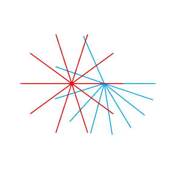
We now compare configurations of line segments stemming from a common origin (Figure 6). The segments’ orientations are sampled uniformly over (, ) in the template, but not in the target (, ). The target is moreover slightly translated. Here, and for the examples that follow, the cost function considers the curves as unlabeled (no correspondence information is used). Formally, this corresponds to considering that the curves are parametrized over the unions of copies of , and using in place of in (15). This choice makes the matching problem significantly harder, creating possible local minima in the cost function. Such local minima actually trap the LDDMM algorithm when using small kernel sizes, and the solution provided in our experiments use a rather large kernel size, , where is the common lengths of the segments. The hybrid model uses combined with (8), the norm corrected for rotations.
As a result of the use of a large kernel in the LDDMM case, the obtained solution does not achieve a perfect transformation of the first segment (the one requiring the largest rotation) which is curved at the end-point of the geodesic (see Figure 7). The segments remain perfectly straight along the geodesic estimated with the hybrid norm (visually at least: an exact transformation of the rays would not be diffeomorphic, but the deviation from a straight line happens below the discretization level chosen for the curves). The effect of the kernel size is also apparent in the estimated transformations, depicted in Figure 6. Similar to the previous examples, the reparametrization of the segments is more pronounced with standard LDDMM.


2.3.4. Half Circles
Our last 2D example is similar to the previous one, using half circles, with various radii, instead of straight lines. We used the rotation- and scale-invariant norm (9) in the hybrid case, and the kernel sizes were and for standard and hybrid LDDMM, being the radius of the largest circle. Both methods do a good job in registering the target to the template, but find different solutions as seen in Figure 8. The LDDMM solution tends to compress the space in the middle of the estimated pattern, while hybrid LDDMM estimates a motion closer to a rotation (which is cheap with the considered norm).


3. Surfaces
The same approach can also be used with surfaces. At high level, not much needs to be modified formally from the curve case, simply letting be the unit disc, or the unit sphere, or any other manifold sharing the topology of the considered surfaces. One can find a large collection of possible choices for in [11, 8, 27, 10]. In the experiment that follows, we used the one of simplest options, letting
| (16) |
where with area measure and Riemannian gradient (it is therefore important that remains an embedding at all times along finite energy paths).
Our example uses the same data as the one presented in Figures 8 and 9 of [3]. It includes three shapes (see Figure 10) who are relatively close to each other (the hippocampus and the amygdala are actually slightly overlapping in the target). If one uses standard LDDMM with a small kernel (, where is the height of the hippocampus), as illustrated in the first row of Figure 11, the diffeomorphism has undesirable properties, crunching parts of the surfaces (such as the front of the hippocampus, the bottom of the entorhinal cortex —which even has a residual spike— and the top of the amygdala) to match the target. With a larger kernel width () the three shapes are transformed as if they formed one single object, resulting in large reparametrization of the surfaces when they move along each other, because points that were nearby initially tend to have similar motions. This is illustrated in the second row of Figure 11. The third row provides the geodesic obtained with the hybrid norm, with the same small kernel width as in the first row, but with (16) penalizing large deformations on the surfaces. In this case, the surfaces move nicely along each other, without requiring large reparametrization, except those required by the change in their respective shapes.


4. Conclusion
Our results illustrate several advantages of combining the standard LDDMM approach with geometrically inspired norms on spaces of curves and surfaces. This very simple concept allows for much more modeling accuracy and flexibility, with a moderate computational impact. This is especially useful when dealing with complex configurations of shapes, as we saw in our examples.
There is clearly still room for future work and development, including the use of higher-order norms for curves and surfaces, and guidelines on which norm to use in specific applications. A version of the method for image matching is another important direction to be explored in the future. Formally, this requires defining , where both and are scalar functions in and using the extra term in the Riemannian norm. One option worth exploring is
where is a “weight function” that depends on , making, for example, deformations more costly in gray/white matter regions than within cerebro-spinal fluid in brain mapping. This will be addressed in future work.
References
- [1] Sylvain Arguillère. The abstract setting for shape deformation analysis and lddmm methods. In Frank Nielsen and Frédéric Barbaresco, editors, Geometric Science of Information: Second International Conference, GSI 2015, Palaiseau, France, October 28-30, 2015, Proceedings, pages 159–167, Cham, 2015. Springer International Publishing.
- [2] Sylvain Arguillère, Emmanuel Trélat, Alain Trouvé, and Laurent Younes. Shape deformation analysis from the optimal control viewpoint. Journal de Mathématiques Pures et Appliquées, 104(1):139–178, 2015.
- [3] Sylvain Arguillère, Emmanuel Trélat, Alain Trouvé, and Laurent Younes. Registration of multiple shapes using constrained optimal control. SIAM Journal on Imaging Sciences, 9(1):344–385, 2016.
- [4] J. Ashburner and K. J. Friston. Voxel based morphometry – the methods. Neuroimage, 11(6):805–821, 2000.
- [5] John Ashburner. A fast diffeomorphic image registration algorithm. Neuroimage, 38(1):95–113, 2007.
- [6] John Ashburner and Karl J Friston. Diffeomorphic registration using geodesic shooting and gauss–newton optimisation. NeuroImage, 55(3):954–967, 2011.
- [7] Brian Avants and James C Gee. Geodesic estimation for large deformation anatomical shape averaging and interpolation. Neuroimage, 23:S139–S150, 2004.
- [8] Martin Bauer and Martins Bruveris. A new Riemannian setting for surface registration setting for surface registration. In Proceedings of the Third International Workshop on Mathematical Foundations of Computational Anatomy-Geometrical and Statistical Methods for Modelling Biological Shape Variability, pages 182–193, 2011.
- [9] Martin Bauer, Martins Bruveris, Stephen Marsland, and Peter W Michor. Constructing reparameterization invariant metrics on spaces of plane curves. Differential Geometry and its Applications, 34:139–165, 2014.
- [10] Martin Bauer, Martins Bruveris, and Peter W Michor. Overview of the geometries of shape spaces and diffeomorphism groups. Journal of Mathematical Imaging and Vision, 50(1-2):60–97, 2014.
- [11] Martin Bauer, Philipp Harms, and Peter W Michor. Sobolev metrics on shape space of surfaces. Journal of Geometric Mechanics (2011), 389-438, pages 389–438, 2011.
- [12] M Faisal Beg, Michael I Miller, Alain Trouvé, and Laurent Younes. Computing large deformation metric mappings via geodesic flows of diffeomorphisms. International journal of computer vision, 61(2):139–157, 2005.
- [13] Yan Cao, Michael I Miller, Raimond L Winslow, and Laurent Younes. Large deformation diffeomorphic metric mapping of vector fields. Medical Imaging, IEEE Transactions on, 24(9):1216–1230, 2005.
- [14] Can Ceritoglu, Kenichi Oishi, Xin Li, Ming-Chung Chou, Laurent Younes, Marilyn Albert, Constantine Lyketsos, Peter van Zijl, Michael I Miller, and Susumu Mori. Multi-contrast large deformation diffeomorphic metric mapping for diffusion tensor imaging. Neuroimage, 47(2):618–627, 2009.
- [15] N. Charon and A. Trouvé. The varifold representation of nonoriented shapes for diffeomorphic registration. SIAM Journal on Imaging Sciences, 6(4):2547–2580, 2013.
- [16] Gary E. Christensen, Richard D. Rabbitt, and Michael I. Miller. Deformable templates using large deformation kinematics. Image Processing, IEEE Transactions on, 5(10):1435–1447, 1996.
- [17] Marc Droske and Martin Rumpf. A variational approach to nonrigid morphological image registration. SIAM Journal on Applied Mathematics, 64(2):668–687, 2004.
- [18] Joan Glaunès, Anqi Qiu, Michael I Miller, and Laurent Younes. Large deformation diffeomorphic metric curve mapping. International journal of computer vision, 80(3):317–336, 2008.
- [19] Monica Hernandez, Salvador Olmos, and Xavier Pennec. Comparing algorithms for diffeomorphic registration: Stationary lddmm and diffeomorphic demons. In 2nd MICCAI Workshop on Mathematical Foundations of Computational Anatomy, pages 24–35, 2008.
- [20] Darryl D Holm, Jerrold E Marsden, and Tudor S Ratiu. The Euler–Poincaré equations and semidirect products with applications to continuum theories. Advances in Mathematics, 137(1):1–81, 1998.
- [21] Darryl D Holm, Alain Trouvé, and Laurent Younes. The Euler-Poincaré theory of metamorphosis. Quarterly of Applied Mathematics, 97:661–685, 2009.
- [22] S. Joshi. Large Deformation Diffeomorphisms and Gaussian Random Fields for Statistical Characterization of Brain Sub-manifolds. PhD thesis, Sever institute of technology, Washington University, 1997.
- [23] Sarang C. Joshi and Michael I. Miller. Landmark matching via large deformation diffeomorphisms. IEEE Transactions on Image Processing, 9:1357–1370, 2000.
- [24] E. Klassen, A. Srivastava, W. Mio, and S. H. Joshi. Analysis of planar shapes using geodesic paths on shape spaces. IEEE Trans. Pattern Anal. Mach. Intell., 26(3):372–383, 2004.
- [25] Arno Klein, Jesper Andersson, Babak A. Ardekani, John Ashburner, Brian Avants, Ming-Chang Chiang, Gary E. Christensen, D. Louis Collins, James Gee, Pierre Hellier, Joo Hyun Song, Mark Jenkinson, Claude Lepage, Daniel Rueckert, Paul Thompson, Tom Vercauteren, Roger P. Woods, J. John Mann, and Ramin V. Parsey. Evaluation of 14 nonlinear deformation algorithms applied to human brain {MRI} registration. NeuroImage, 46(3):786 – 802, 2009.
- [26] Hi L Krall and Orrin Frink. A new class of orthogonal polynomials: The bessel polynomials. Transactions of the American Mathematical Society, 65(1):100–115, 1949.
- [27] Sebastian Kurtek, Eric Klassen, Zhaohua Ding, Sandra W Jacobson, Joseph L Jacobson, Malcolm J Avison, and Anuj Srivastava. Parameterization-invariant shape comparisons of anatomical surfaces. IEEE Transactions on Medical Imaging, 30(3):849–858, 2011.
- [28] P. W. Michor and D. Mumford. Riemannian geometries on spaces of plane curves. J. Eur. Math. Soc., 8:1–48, 2006.
- [29] P. W. Michor and D. Mumford. An overview of the Riemannian metrics on spaces of curves using the Hamiltonian approach. Applied and Computational Harmonic Analysis, 23(1):74–113, 2007.
- [30] Michael I Miller, Alain Trouvé, and Laurent Younes. Geodesic shooting for computational anatomy. Journal of mathematical imaging and vision, 24(2):209–228, 2006.
- [31] Michael I. Miller and Laurent Younes. Group actions, homeomorphisms, and matching: A general framework. International Journal of Computer Vision, 41(1-2):61–84, 2001.
- [32] Dimitrios Pantazis, Richard M Leahy, Thomas E Nichols, and Martin Styner. Statistical surface-based morphometry using a nonparametric approach. In Biomedical Imaging: Nano to Macro, 2004. IEEE International Symposium on, pages 1283–1286. IEEE, 2004.
- [33] Laurent Risser, F Vialard, Robin Wolz, Maria Murgasova, Darryl D Holm, and Daniel Rueckert. Simultaneous multi-scale registration using large deformation diffeomorphic metric mapping. Medical Imaging, IEEE Transactions on, 30(10):1746–1759, 2011.
- [34] Martin Styner, Ipek Oguz, Shun Xu, Christian Brechbühler, Dimitrios Pantazis, James J Levitt, Martha E Shenton, and Guido Gerig. Framework for the statistical shape analysis of brain structures using spharm-pdm. The insight journal, 1071:242, 2006.
- [35] Alain Trouvé and Laurent Younes. Metamorphoses through Lie group action. Foundations of Computational Mathematics, 5(2):173–198, 2005.
- [36] Tom Vercauteren, Xavier Pennec, Aymeric Perchant, and Nicholas Ayache. Diffeomorphic demons: Efficient non-parametric image registration. NeuroImage, 45(1):S61–S72, 2009.
- [37] Anthony Yezzi and Andrea Mennucci. Metrics in the space of curves. arXiv preprint math/0412454, 2004.
- [38] L. Younes, P. Michor, J. Shah, and D. Mumford. A metric on shape spaces with explicit geodesics. Rend. Lincei Mat. Appl., 9:25–57, 2008.
- [39] Laurent Younes. Computable elastic distances between shapes. SIAM Journal on Applied Mathematics, 58(2):565–586, 1998.
- [40] Laurent Younes. Jacobi fields in groups of diffeomorphisms and applications. Quarterly of applied mathematics, 65(1):113–134, 2007.
- [41] Laurent Younes, Felipe Arrate, and Michael I Miller. Evolutions equations in computational anatomy. NeuroImage, 45(1):S40–S50, 2009.