An Efficient Algorithm To Compute The Colored Jones Polynomial
The colored Jones polynomial is a knot invariant that plays a central role in low dimensional topology. We give a simple and an efficient algorithm to compute the colored Jones polynomial of any knot. Our algorithm utilizes the walks along a braid model of the colored Jones polynomial that was refined by Armond from the work of Huynh and Lê. The walk model gives rise to ordered words in a -Weyl algebra which we address and study from multiple perspectives. We provide a highly optimized Mathematica implementation that exploits the modern features of the software. We include a performance analysis for the running time of our algorithm. Our implementation of the algorithm shows that our method usually runs in faster time than the existing state-of the-art method by an order of magnitude.
1. Introduction
Let be a knot in and be a positive integer. The colored Jones polynomial (CJP) denoted and defined in [45, 48, 49] is a Laurent polynomial with integer coefficients in the variable . The label stands for the coloring, i.e., the irreducible representation of from which it is calculated. The polynomial is the original Jones polynomial [31]. The colored Jones polynomial and its generalizations [18, 50, 30, 33] play an important role in low-dimensional topology, in particular through its connection to the volume conjecture [45, 32, 46]. Since its discovery, the Jones polynomial has lead major discoveries [53, 52] and seen major advances in various areas in low-dimensional topology [37, 35, 13, 6, 38, 20, 36]. Moreover, recent years have witnessed considerable developments that established multiple connections between the colored Jones polynomial and number theory. See for instance [39, 14, 22, 9, 41, 4, 23, 8]. The coefficients of the colored Jones polynomial have been proven to give rise to Ramanujan theta and false theta identities [4, 15]. See also [19] and the references therein for more about the history and development of the colored Jones polynomial.
Computing the colored Jones polynomial is a highly non-trivial task. Much of the literature on computing the colored Jones polynomial is devoted to giving quantum algorithms of this polynomial. The existence of an efficient algorithm for approximating was implied in the work of Freedman, and Kitaev [16]. Later an explicit quantum algorithm for approximating the Jones polynomial was given in [2] and extended later in [54, 1]. More on the quantum computation of the Jones polynomial can be found in [34, 47].
One of the earlier classical algorithms to compute the colored Jones polynomial was given in [42] by Masbaum and Vogel where the skein theory associated to the Kauffman bracket skein module was utilized. This algorithm can be considered as an extension of the Kauffman bracket which in turn can be used in algorithms to compute the original Jones polynomial. Masbaum and Vogel’s algorithm however relies on certain diagrammatic manipulations that require special handling for each knot making it hard to obtain an efficient general implementation. In [20] the -holonomicity of the colored Jones polynomial was proven and this in turn can be used to compute the colored Jones polynomial. Bar-Natan’s Mathematica package KnotTheory [7] implements this to compute the colored Jones polynomial. The algorithm however is mostly feasible for knots with small crossing number and color . The other commonly used publicly available implementation for the Jones polynomial that we are aware of is SnapPy [12], but this implementation however only handles the Jones polynomial, i.e., when .
Explicit formulas for of the colored Jones polynomial of the double twist knots can be found in [43] and for torus knots in [44]. Moreover, a difference equation for torus knots is given in [24]. The complexity of the Jones polynomial of alternating links is studied in [28]. More on the computational complexity of the Jones polynomial and its generalization can be found in [17].
In this article we give an efficient classical algorithm to compute the colored Jones polynomial for any knot based on the quantum determinant formula suggested by Huynh and Lê [25]. In particular we consider a walk along a braid interpretation of the evaluation of this quantum determinant that was developed by Armond [5], in light of Jones’ interpretation of the Burau Representation [29]. This walk model gives rise to an ordered word in a -Weyl algebra which is studied from multiple perspectives. The algorithm converts each word to a standard word defined in this paper and then evaluates each word to a Laurent polynomial. To minimize the number of words needed for evaluation, we utilize a structural theorem regarding the set of walks on braids. Along with our algorithm we provide a highly optimized Mathematica [26] implementation that exploits several modern features and functionalities in Mathematica.
2. Preliminaries
We give a quick review here of braid groups as it will be needed in later sections.
2.1. Braid Group
The input of the colored Jones polynomial algorithm we present here is a braid whose closure forms a knot. Alexander’s theorem [3] assures that any knot can be realized as the closure of a braid in this manner.
Let denote the manifold with boundary . Fix points on the top of and points on the bottom. A braid on strands is a curve embedded in and decomposed into arcs such it meets orthogonally in exactly points and where no arc intersects any horizontal plane more than once. A braid is usually represent a planar projection or a braid diagram. In the braid diagram we make sure that each crossing the over strand is distinguishable from the under-strand by creating a break in the under-strand. Figure 1 shows an example of a braid diagram on strands.

The set of all braids has a group structure with multiplication as follows. Given two strand braids and the product of these braids, is the braid given the by vertical concatenation of on top of . As in Figure 2.

The group structure of follows directly from this. The braid group on strands can be described algebraically in terms of generators and relations using Artin’s presentation. In this presentation, the group is given by the generators :
subject to the relations:
- (1)
For all : .
- (2)
For : .
- (3)
For all :
The correspondence between the pictorial definition of the braid group and the algebraic definition is given by sending the generator to the picture illustrated in Figure 3.

The braid closure of a braid is given by joining the points on the top of to the points on the bottom by parallel arcs as follows:

3. Walks on Braids
In [25] Lee suggested a realization of the colored Jones polynomial as the inverse of the quantum determinant of an almost quantum matrix. The entries of this matrix live in the -Weyl algebra. The quantum determinant version of the colored Jones polynomial admits a walks along a braid model described by Armond in [4]. In this section we review this walk model and define the necessary terms that will be utilized in the algorithm section.
Recall that all knots can be realized as the closure of a braid [3]. Moreover, given a knot, this braid can be computed using Yamada-Vogel’s Algorithm [55, 51]. The algorithm utilized here takes a braid as input,which is uniquely determined by the braid sequence , described next.
Let be a braid in given by the braid word:
| (3.1) |
The braid sequence of the braid is a finite sequence of pairs , and . For instance the braid sequence of the braid is . Conversely, a sequence of pairs , where and gives rise to a braid in . We recommend the reader to the work of T. Gittings [21] or the tables of C. Livingston [11] for collections of minimal braid sequences.
We will denote by the braid associated to the sequence . For the rest of this paper we will refer to the braid and its associated braid sequence interchangeably. Moreover, we will refer to the pair as a crossing in the braid.
A path on a braid from a strand , counting up from left to right as in Figure 3, to a strand , is defined as follows. We start at the bottom at the strand of the braid and we march to the top. Whenever arriving at an over-crossing we can either jump down to the lower strand or continue along the same strand. We continue in this manner until we reach the top of the braid at the strand. Note that when a path goes from the bottom to the top on a braid it passes some collection of crossings of . At a crossing we encode this passage by the following conventions:
- (1)
If a path jumps down at , we assign that crossing the weight .
- (2)
If a path follows the bottom strand at , we assign that crossing the weight .
- (3)
If a path follows the top strand at , we assign that crossing the weight .
Figure 5 illustrates the three types possible behavior of a path at a crossing and the weights assigns to local path in each case.

The weights , and will be given additional meaning in section 4. The weight of a single strand path is the product of the weights of its crossings, the weight of a path is the product from bottom right to left of the weights of each individual strand path. Notice that the weights are not allowed to commute in general. This is elaborated on in section 4.
Remark 3.1.
It is important to notice that we read the braid in two different directions. When we read a path on a braid we read it from bottom to top. Whereas when we read the braid word as product of braid group generators we read that from top to bottom. See example 8.3 for an illustration.
A walk along the braid in consists of the following data :
- (1)
A set .
- (2)
A permutation of .
- (3)
A collection of paths on with exactly one path in from strand to strand , for each .
We denote by the number of inversions in the permutation , i.e. the number of pairs such that . Then every walk is assigned a weight defined as times the product of the weights of the paths in the collection . A walk is said to be simple if no two paths in the collection traverse the same point on the braid. Simple walks are desirable for computational reasons and we will consider only them for algorithmic efficiency. A stack of walks is an ordered collection of walks. Finally, the weight of a stack is the product of the weights of its walks.
4. Algebra of the deformed Burau matrix
Let . For each braid we define an -algebra , where is the sequence , as follows. We associate to every a the letters : , and . The algebra is the -algebra freely generated by the set subject to the following commutation relations:
| (4.1) | ||||||||
| (4.2) |
Here can be thought of as a skew-commutator for each algebra, but for any two elements where we have:
| (4.3) |
The relationship between the walks introduced in the previous section and elements of the algebra will be made explicit in section 8. For the rest of the paper we fix to be the sequence and refer to the algebra associated to by as defined above.
4.1. Right Quantum Words in
Relations 4.1, 4.2 and 4.3 are utilized in our algorithm to convert any word in the algebra to a standardized word that will facilitate the computation of the colored Jones polynomial.
A word in is a finite product of elements from . A monomial in is a product where and is a word in . A word in is said to be a right quantum if it has the form:
where
| (4.4) |
| (4.5) |
such that , and . By convention the empty word will be assumed to be right quantum. Algorithm 1 summarizes the first step in the conversion of a word to a right quantum word.
Now let be an arbitrary word in . Using the relations 4.1, 4.2 and 4.3 we can write:
| (4.6) |
where is a right quantum word and is an integer. We call the word the quantum word associated with the word . Using this convention, we define the word vector of as the sequence of integers :
| (4.7) |
Note here that the exponents , and are simply the number of times each variable , and occurs in the word . Hence these numbers can be computed simply without any consideration of the algebra relations. The same holds for determining the exponents , and . On the other hand, in order to compute the exponent the word must be converted to right quantum form using the algebra relations. We will come back to this fact later while describing the main algorithm.
Remark 4.1.
Since any monomial is a scalar multiple of a word, the definition of quantum word can be also defined on monomials. For this reason the technical difference between words and monomials is not essential and in our discussion below we use these two terms interchangeably.
Remark 4.2.
Note that the weight of an arbitrary walk along a braid is simply a word in . For our purposes, we are not interested in all words in , instead we are merely concerned about words that can be realized as a weight of walk or a product of such words. This fact will be utilized in Section 9.2 in order to reduce the calculations needed for evaluation of these words as elements in .
5. The Evaluation Map
Here we introduce the -evaluation map that operates on elements in and returns a polynomial in . Since the purpose of this paper is to give an algorithm to compute the colored Jones polynomial we will solely give the axioms that are necessary to calculate the map . The reader further interested in this map is referred to the paper [40] for an equivalent set of axioms and their full construction.
Definition 5.1.
For the function is defined via the following axioms:
- (1)
For any ,
- (2)
For any and ,
- (3)
For any two monomials that are separable, which occurs when the monomial only contains the letters with and the monomial has only letters with where , we have
- (4)
- (5)
.
Now let be an arbitrary element in . We are interested in the explicit evaluation of . To this end, observe first that the element can be written in the form where is a monomial in for . The computation of the colored Jones polynomial in our algorithm relies essentially on the computation of . In the case of the colored Jones polynomial the element is not just an arbitrary element in the algebra . Specifically, the set possesses a structure with respect to the evaluation map that allows for its efficient computation. We will introduce this structure along with the method to evaluate on the special types of elements in Section 9 after we give the definition of the colored Jones polynomial in terms of the evaluation map.
6. Quantum determinant
Let be elements of the noncommutative ring A matrix is said to be right quantum if :
- (1)
- (2)
- (3)
An matrix is said to be right quantum if all its submatrices are right quantum. If is a right quantum matrix then the quantum determinant of is given by :
| (6.1) |
where is the number of inversions in the permutation .
Let be an matrix and let . The matrix is the submatrix of obtained by selecting the rows and columns of that correspond to the set . Note that if is right quantum then is also right quantum. If is a right quantum matrix then define by
| (6.2) |
7. Deformed Burau Matrix
The deformed Burau matrix associated to a braid is defined similar to the Burau Matrix [10]. Define the matrices
To every braid generator in Artin’s standard presentation we associate an right-quantum matrix which is the identity matrix except at the submatrix of rows , and columns , which we replace by . The matrix is the same as the matrix but , and are replaced with , and respectively. The matrix is called the deformed Burau matrix associated with the generator . For a braid given as , the deformed Burau matrix is defined by the multiplication of its corresponding deformed Burau matrices: . The reduced deformed Burau matrix is obtained from by dropping both the first row and first column. Note that is a right quantum matrix, so is as well.
Looking back at Figure 5, one can see how for a positive crossing the weight corresponds to a path moving from the bottom of the diagram to the top by following from position on the overcrossing strand and jumping to the position on the undercrossing strand, the weight corresponds to a path that moves from the position to the position by following the undercrossing strand and the weight corresponds to a path that moves from the position to the position by following the overcrossing strand. Similarly, for negative crossings, the matrix elements of the matrix, , correspond to the transition from the bottom strand (column) of a crossing to the top strand (row).
8. The Colored Jones Polynomial
In this section we give the definition of the colored Jones polynomial using the Burau representation we described in the previous section. We recall some facts about the Jones and colored Jones polynomial first. The Jones polynomial is a Laurent polynomial knot invariant in the variable with integer coefficients. The Jones polynomial generalizes to an invariant of a knot colored by the irreducible representation of and normalized so that , where denotes the unknot. Note that this is the unframed normalized version of the colored Jones polynomial. The original Jones polynomial corresponds to the case . In [25] it was shown that the colored Jones polynomial of a knot can be computed in terms of the quantum determinant of the deformed Burau representation of a braid with . We recall the statement of this theorem here since it will be utilized in our algorithm.
Theorem 8.1 ([25, Theorem 1]).
Suppose the closure in the standard way of the -strand braid is a knot . Then for any positive integer we have
where is the writhe of the knot and is the number of strands in its braid representation.
Remark 8.2.
In [4] Armond interpreted the polynomial from equation 6.2 as a sum of the weights of walks on with . Noting that this deformed Burau representation corresponds to removing the first strand as either a starting or ending point, but allowing it to be traversed midbraid. In this interpretation, it is natural to understand higher powers as a stack of superimposed walks with . We elaborate on the idea of a stack of walks further in section 9.2.
Example 8.3.
Let be the braid in ( see Figure 6).

The closure of gives the figure eight knot. Moreover, and . Computing the deformed Burau representation of gives the right-quantum matrix:
Hence the reduced Burau matrix is given by :
| (8.3) |
Using the quantum determinant formula one obtains the following summation of walks:
| (8.4) | ||||
Thus the colored Jones polynomial is given by:
9. Evaluation of the Map
A computation bottleneck in the main algorithm of the CJP lies in evaluating for elements From the Theorem 8.1 point of view it seems that this computation comes down to computing where each is obtained from the quantum determinant. However this naive approach is far from efficient. Our initial implementation using this interpretation could not practically perform calculations for some knots of index 10. But, as mentioned in Remark 8.2 the polynomial can be understood as a sum of the weights of walks on the braid. In this section we illustrate how this sum can be simplified to only require simple walks. In other words, all non-simple walks can be ignored from the computation of entirely.
For simplicity we will be considering the evaluation of on an arbitrary element . We then focus on the special cases where is solely generated by walks. To this end, let
where each is an individual monomial in for . The polynomial evaluation of simplifies to:
| (9.1) |
following axiom of the evaluation map . Moreover, any monomial can be written as where is a word and . Hence by axiom 2 of the evaluation map we have
Hence the problem of evaluating is reduced to the calculation of on each word in .
9.1. Evaluation of Words in
We now describe the evaluation of an arbitrary word in .
Lemma 9.1.
Let be an arbitrary word in and let
be the word vector of . Then
Proof.
Equation 4.6 implies that , where is an integer and is a right quantum word. Hence, by axiom of the evaluation map ,
Moreover, since is a right quantum word, . However, the words and are separable. Hence, axiom of implies that:
By identities 4.4 and 4.5, and axioms and of the function , we obtain the result. ∎
Lemma 9.1 nearly allows any word to be evaluated explicitly by simply counting the number of times each of the , and occurs in the word and applying the formula. The only problem is computing of the power which requires the algebra relations as we mentioned before. From relations 4.1, 4.2 and 4.3 we find that the can be computed given the following numbers :
- (1)
The total of the number of times each appears to the left of each in the word .
- (2)
The total of the number of times each appears to the left of each in the word .
- (3)
The total of the number of times each appears to the left of each in the word .
- (4)
The total of the number of times each appears to the left of each in the word .
- (5)
The total of the number of times each appears to the left of each in the word .
We will use the following convention to refer to the previous numbers. Let be a word and and be two letters in . We denote by the total of the number of times each letter appears to the left of the letter in the word . When is clear from the context we will use the notation instead. Using this convention and the relations 4.1, 4.2 and 4.3 we can write :
| (9.2) |
Algorithm 2 summarizes this process of calculating the word vector, of each word in .
9.2. Efficient Evaluation of
As before, let in , where is a monomial for . We denote by the set of monomials coming from walks in . For words coming from stacks of walks, we denote the walks of stack height by , so that each corresponds to the walk in . We are interested in the efficient computation of . As previously emphasized, this potentially infinite sum is a bottleneck for computing the algorithm. We employ two techniques for minimizing the number of the monomials in the set where we need to evaluate the function , which we describe next.
9.2.1. Utilizing the Property of the CJP with Respect to the Mirror Image of Knots
Let and be two knots that are mirror images of each other. Let and be two braids with and . It is known that the colored Jones polynomial satisfies the property . We can utilize this fact to reduce the number of computations using a simple strategy. By first computing the number of simple walks in and computing the number of simple walks in the program chooses to work with the one that has fewer simple walks to run the CJP computation.
Computing the simple walks of both the braid and its mirror image, takes some additional time forcing the computation of the colored Jones polynomial to be slower than if only one set of simple walks were considered. However, this is only true for small choices of . As mentioned earlier, the number of simple walks affects the performance of the algorithm more than any other parameter. By choosing the braid representation that minimizes this number, our algorithm significantly reduces the number of computations done as the number of colors increases.
9.2.2. The Duplicate Reduction Lemma
Another large gain in computational efficiency is created by removing walks which have either zero contribution to the final sum or by deleting pairs of walks that have zero net contribution to the final sum. For computing it is useful to divide the set of monomials from walk weights into the set of weights of simple and non-simple walks on the braid . Due to [5, Lemma 4], stated below in Lemma 9.3, we only need to consider simple walks from the set . The non-simple walks occur in canceling pairs that have zero net value when evaluated with the map .
Lemma 9.3 (Duplicate Reduction [5, Lemma 4]).
- (1)
For any monomial, , corresponding to the weight of a non-simple walk, there is another monomial whose weight evaluates to the negative of the original monomial.
- (2)
For any monomial, , corresponding to the weight of a stack of simple walks, , with , where the stack of walks traverses the same point on different levels, the evaluation of that weight will be zero.
Definition 9.4.
Two monomials and , which have the same letters in any order are said to be paired if .
Paired monomials help reduce the calculations needed for as follows. By Lemma 9.3.1 any non-simple walk, is paired with a walk as in Definition 9.4 so that . Furthermore, as we will discuss in Remark 9.6, for paired walks and any walk , . So all non-simple walks can be ignored from the calculation of and furthermore in part 2 of the lemma, any stack of walks in can be ignored from the calculation as well, so long as one of the is non-simple.
Definition 9.5.
A monomial is said to be zero -evaluated if
In example 8.3, the non-simple walks and are paired in equation 8.4. Applying Definition 9.5 to these same walks for and we see that they are both zero 2-evaluated, but that neither is zero 3-evaluated. As with paired walks, given a zero -evaluated walk , where , then for any walk .
Remark 9.6.
To be precise, given a braid , we define , a subalgebra of . The algebra represents exactly the minimal subalgebra of containing the monomials needed by our algorithm to evaluate the colored Jones polynomial. In this subalgebra the -span of the set of zero -evaluated words forms an ideal. Similarly, the span of the set of monomials corresponding to the weights of paired walks in forms an ideal in . However, further information regarding these ideals does not further our computational aims so we omit the details.
Remark 9.7.
All non-simple walks are zero 2-evaluated. If , then there exists a in so that both and and for all , and any in as above. This allows the duplicate reduction lemma to be implemented with a single algorithm.
Since non-simple walks will not be included in our computation we can ignore those walks completely from the determinant calculation. This is handled by Algorithms 3 and 4 simultaneously. Algorithm 3 focuses on removing nonsimple, paired walks.
Algorithm 4 assists in the implementation of algorithm 3, with orders of magnitude speed increases for determining the reduced Burau representation. It takes as input a list of walks and returns the sublist containing the walks that do not -evaluate to zero.
10. Description of the Main Algorithm
The main algorithm takes as input a knot , given as the closure of a braid , a positive integer and , which is either a commutative variable or a complex number. The braid can be chosen to be any braid with , though we recommend using the minimal forms described above for efficiency. The output of the main algorithm is the colored Jones polynomial . The algorithm starts by initiating the CJP to . It then checks if the input braid is the empty braid, returning if this is the case. Otherwise the algorithm checks the number of simple walks of the braid and its mirror image and retains whichever form had the minimal number of simple walks for the rest of the computation. After that the algorithm creates a while loop. This while loop calculates for and adds those evaluations. The while loop terminates when for some . When this happens the algorithm exits the while loop and returns after converting it into a Laurent polynomial.
11. Implementation and Performance
In this section we give a brief description of our Mathematica implementation of the algorithms before we discuss the performance of algorithm 5 on the knot table.
11.1. Implementation
For our implementation we used Mathematica [26] to handle the symbolic computation of the algorithm. For noncommutative multiplication in the algebra , we used NCAlgebra package for Mathematica [27]. In particular, we relied on the NCPoly data structure, which allowed the majority of computations to be done using integer arithmetic rather than symbolic calculations, providing significant speed gains. Additionally we take advantage of Mathematica’s memoization techniques and functional programming structure for additional efficiency gains in algorithms 1 and 3, and with helper functions to algorithm 2. In algorithm 4 the inner for loop is replaced with code that utilizes Mathematica’s pattern recognition features, rather than using a constantly reindexing list suffering frequent object removal. Intensive pieces of code are reduced to C-compiled parallelized functions where possible. Thus the code contains two implementations of Algorithms 1, 2, and 4, one using C-code and a commented out version using pure Mathematica code, for use if your computer does not include a C-compiler.
In implementing Algorithm 5 the return step includes two features. The community is often interested in evaluating the color Jones polynomial at roots of unity, so before returning the polynomial it evaluates at if a complex variable was supplied rather than an indeterminant. Additionally, the initial output is often a dense collection of sums and products. We add two steps into the code to render the data into Laurent polynomials before output. All the data collected in the charts below includes this extra step of simplifying the information into this form. The additional requirement to return Laurent polynomials increases run times by up to an order of magnitude. We have chosen to include this in our performance evaluations as we believe most users will wish to render the data into a simpler form before using it.
The software for the CJP polynomial is available for public use and currently can be downloaded from the GitHub repository: github.com/jsflevitt/color-Jones-from-walks.
11.2. Performance
In order to test the efficiency of our method we performed several tests on the knot table with knots whose crossing numbers are less than or equal to 12. Our tests were performed on a 3.20 GHz Intel Core i5 with 8.0 Gb of memory on the macOS platform. As we mentioned earlier the computational time of algorithm 5 relies mainly on the number of simple walks of the input knot. For this reason we test this algorithm with respect to the number of simple walks. Specifically, recall that algorithm 5 computes the minimal number of the simple walks between the knot and its mirror and then it performs the computations with the knot which has fewer number of simple walks. For this reason, the running time of 5 is compared against the number of simple walks between the knot and its mirror image. This performance is shown in Figure 7 for the all knots in the knots table with number of crossings less than or equal 12. From Figure 7 one can observe that there are several knots that share the same number of simple walks.

The correlation between the number of crossings of a knot and the number of simple walks is not immediate from the definition. Moreover, Algorithm 4 makes non-linear reductions to the number of final walks needed to compute the colored Jones polynomial in Algorithm 5. To obtain a better understanding of the growth of the number of simple walks as the number of crossing increases we give Figure 8 where the number of simple walks needed to compute the colored Jones polynomial is plotted with respect to the number of crossings. Figure 8 suggests that average of number of simple walks is bounded by , where is the number of crossings. Although proving this claim requires a more thorough analysis, starting with understanding how to find the minimal braid word for any knot .

The performance of our algorithm as the number of color increases is shown in Figure 9. Here we compute the colored Jones polynomial for each color between and three times for each knot and compare the average running time with respect to the number of simple walks. We show the performance of the algorithm on individual knots as we increase the number of colors in Figure 12 and elaborate on this when we compare our algorithm with the algorithm provided in KnotTheory package [7].

11.3. Number of Walks and The Duplicate Reduction Lemma
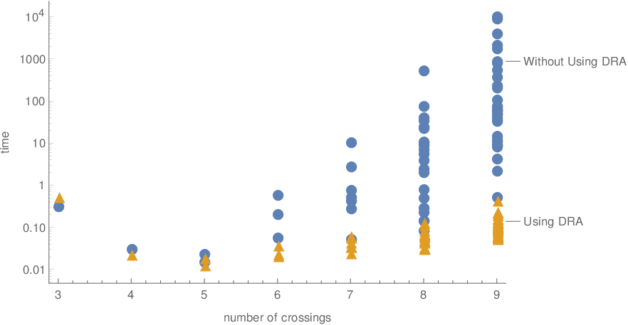
To show the impact the Algorithm 4 on the running time we conducted several tests. We run our experiments on the first on all knots in the knot table with crossings less than or equal to 9. For all these knots we computed the number of walks in in . Having the number of simple walks in minimal is critical because our method computes which for all such that . Our comparison goes as follows. For each knot with number of crossing between 3 and 9 we compute the number of walks in in two different ways : (1) with the utilization of Algorithm 4 and (2) without using that Algorithm. Figure 10 shows the impact of using Algorithm 10 on the total number of walks that is needed to compute the colored Jones polynomial.

In Figure 11 we did we show impact of utilization Algorithm 4 on the running time. Note that using Algorithm 4 impacts the running time of the Algorithm 5 by an order of magnitude. In our experimentation some knots with 9 crossings number did not even run on our machine without the utilization of Algorithm 4 in the Algorithm 5.
11.4. Comparing the running time with the KnotTheory Package
We also run our algorithm against the implementation of the colored Jones polynomial provided in KnotTheory package [7]. Figure 12 shows the running time comparison between our method and the KnotTheory package REngine method for the first 28 knots in the knot table.
The circular dots represent the KnotTheory Package running time while the triangular dots represent our algorithm’s running time. The figure shows that our method is faster by an order of magnitude for most knots shown in the figure. As a final note, we have yet to overflow memory while running our algorithm, while the REngine calculation occasionally crashed for this reason preventing a fuller comparison.

12. Acknowledgment
The authors would like to thank Cody Armond and Kyle Istvan for many useful conversations while writing this paper. We also would like to thank Matt Hogancamp for several suggestions that improved the paper’s clarity. The second author was partially supported by the National Science Foundation (grant no. DMS-1764210). Finally we thank Iris Buschelman, Ina Petkova and Katherine Lee Pierret Perkins for their assistance.
References
- [1] (2011) The bqp-hardness of approximating the jones polynomial. New Journal of Physics 13 (3), pp. 035019. Cited by: §1.
- [2] (2009) A polynomial quantum algorithm for approximating the jones polynomial. Algorithmica 55 (3), pp. 395–421. Cited by: §1.
- [3] (1923) A lemma on systems of knotted curves. Proceedings of the National Academy of Sciences 9 (3), pp. 93–95. Cited by: §2.1, §3.
- [4] (2011) Rogers-ramanujan type identities and the head and tail of the colored jones polynomial. arXiv preprint arXiv:1106.3948. Cited by: §1, §3, Remark 8.2.
- [5] (2014) Walks along braids and the colored jones polynomial. Journal of Knot Theory and Its Ramifications 23 (02), pp. 1450007. Cited by: §1, §9.2.2, Lemma 9.3.
- [6] (1996) On the melvin–morton–rozansky conjecture. Inventiones mathematicae 125 (1), pp. 103–133. Cited by: §1.
- [7] The Knot Atlas. External Links: Link Cited by: §1, Figure 12, §11.2, §11.4.
- [8] (2016) The colored jones polynomial of singular knots. New York J. Math 22, pp. 1439–1456. Cited by: §1.
- [9] (2017) Q-series and tails of colored jones polynomials. Indagationes Mathematicae 28 (1), pp. 247–260. Cited by: §1.
- [10] X, braids, links, and mapping class groups. Ann. of Math. Studies 82. Cited by: §7.
- [11] (December 29, 2017) Knotinfo: table of knot invariants, http://www.indiana.edu/ knotinfo. Cited by: §3.
- [12] SnapPy, a computer program for studying the geometry and topology of -manifolds. Cited by: §1.
- [13] (2006) On the head and the tail of the colored jones polynomial. Compositio Mathematica 142 (5), pp. 1332–1342. Cited by: §1.
- [14] (2017) Pretzel knots and -series. Osaka Journal of Mathematics 54 (2), pp. 363–381. Cited by: §1.
- [15] (2018) Foundations of the colored jones polynomial of singular knots. Bull. Korean Math. Soc. Cited by: §1.
- [16] (2002) Simulation of topological field theories by quantum computers. Communications in Mathematical Physics 227 (3), pp. 587–603. Cited by: §1.
- [17] (1998) P/np, and the quantum field computer. Proceedings of the National Academy of Sciences 95 (1), pp. 98–101. Cited by: §1.
- [18] (1985) A new polynomial invariant of knots and links. Bulletin of the American Mathematical Society 12 (2), pp. 239–246. Cited by: §1.
- [19] (2012) Guts of surfaces and the colored jones polynomial. Vol. 2069, Springer. Cited by: §1.
- [20] (2005) The colored jones function is q-holonomic. Geometry & Topology 9 (3), pp. 1253–1293. Cited by: §1, §1.
- [21] (2004) Minimum braids: a complete invariant of knots and links. arXiv preprint math. External Links: ISSN 0401051/ Cited by: §3.
- [22] (2016) The tail of a quantum spin network. The Ramanujan Journal 40 (1), pp. 135–176. Cited by: §1.
- [23] (2017) The colored kauffman skein relation and the head and tail of the colored jones polynomial. Journal of Knot Theory and Its Ramifications 26 (03), pp. 1741002. Cited by: §1.
- [24] (2004) Difference equation of the colored jones polynomial for torus knot. International Journal of Mathematics 15 (09), pp. 959–965. Cited by: §1.
- [25] (2007) On the colored jones polynomial and the kashaev invariant. Journal of Mathematical Sciences 146 (1), pp. 5490–5504. Cited by: §1, §3, Theorem 8.1, §8.
- [26] Mathematica, Version 11.2. Note: Champaign, IL, 2017 Cited by: §1, §11.1.
- [27] A mathematica package for noncommutative calculations. Note: NCAlgebra 4.0 Cited by: §11.1.
- [28] (1990) On the computational complexity of the jones and tutte polynomials. In Mathematical proceedings of the cambridge philosophical society, Vol. 108, pp. 35–53. Cited by: §1.
- [29] (1987) Hecke algebra representations of braid groups and link polynomials. Annals of Mathematics, pp. 335–388. Cited by: §1.
- [30] (1990) Hecke algebra representations of braid groups and link polynomials. In New developments in the theory of knots, pp. 20–73. Cited by: §1.
- [31] (1997) A polynomial invariant for knots via von neumann algebras. In Fields medallists’ lectures, pp. 448–458. Cited by: §1.
- [32] (1997) The hyperbolic volume of knots from the quantum dilogarithm. Letters in Mathematical Physics 39 (3), pp. 269–275. Cited by: §1.
- [33] (1990) An invariant of regular isotopy. Transactions of the American Mathematical Society 318 (2), pp. 417–471. Cited by: §1.
- [34] (2002) Quantum computing and the jones polynomial. CONTEMPORARY MATHEMATICS 305, pp. 101–138. Cited by: §1.
- [35] (2005) Categorifications of the colored jones polynomial. Journal of Knot Theory and its Ramifications 14 (01), pp. 111–130. Cited by: §1.
- [36] (2000) Integrality and symmetry of quantum link invariants. Duke Mathematical Journal 102 (2), pp. 273–306. Cited by: §1.
- [37] (1905) On the aj conjecture for knots. Indiana University Mathematics Journal 64 (4). Cited by: §1.
- [38] (2006) The colored jones polynomial and the a-polynomial of knots. Advances in Mathematics 207 (2), pp. 782–804. Cited by: §1.
- [39] (2018) A trivial tail homology for non-a–adequate links. Algebraic & Geometric Topology 18 (3), pp. 1481–1513. Cited by: §1.
- [40] (2010) Introduction to topological manifolds. Vol. 940, Springer Science & Business Media. Cited by: §5.
- [41] (2013) The bailey chain and mock theta functions. Advances in Mathematics 238, pp. 442–458. Cited by: §1.
- [42] (1994) 3-valent graphs and the kauffman bracket. Pacific Journal of Mathematics 164 (2), pp. 361–381. Cited by: §1.
- [43] (2003) Skein-theoretical derivation of some formulas of habiro. Algebraic & Geometric Topology 3 (1), pp. 537–556. Cited by: §1.
- [44] (1995) The coloured jones function and alexander polynomial for torus knots. In Mathematical proceedings of the cambridge philosophical society, Vol. 117, pp. 129–135. Cited by: §1.
- [45] (2001) The colored jones polynomials and the simplicial volume of a knot. Acta Mathematica 186 (1), pp. 85–104. Cited by: §1.
- [46] (2011) An introduction to the volume conjecture. Interactions between hyperbolic geometry, quantum topology and number theory 541, pp. 1–40. Cited by: §1.
- [47] (2009) Experimental approximation of the jones polynomial with one quantum bit. Physical review letters 103 (25), pp. 250501. Cited by: §1.
- [48] (1990) Ribbon graphs and their invaraints derived from quantum groups. Communications in Mathematical Physics 127 (1), pp. 1–26. Cited by: §1.
- [49] (1988) The yang-baxter equation and invariants of links. Inventiones mathematicae 92 (3), pp. 527–553. Cited by: §1.
- [50] (2016) Quantum invariants of knots and 3-manifolds. Vol. 18, Walter de Gruyter GmbH & Co KG. Cited by: §1.
- [51] (1990) Representation of links by braids: a new algorithm. Commentarii Mathematici Helvetici 65 (1), pp. 104–113. Cited by: §3.
- [52] (1988) 2+ 1 dimensional gravity as an exactly soluble system. Nuclear Physics B 311 (1), pp. 46–78. Cited by: §1.
- [53] (1989) Quantum field theory and the jones polynomial. Communications in Mathematical Physics 121 (3), pp. 351–399. Cited by: §1.
- [54] (2006) The jones polynomial: quantum algorithms and applications in quantum complexity theory. arXiv preprint quant-ph. External Links: ISSN 0603069/ Cited by: §1.
- [55] (1987) The minimal number of seifert circles equals the braid index of a link. Inventiones mathematicae 89 (2), pp. 347–356. Cited by: §3.