Two Metropolis-Hastings algorithms for posterior measures with non-Gaussian priors in infinite dimensions

Bamdad Hosseini Email: bamdadh@caltech.edu Address: Department of Computing & Mathematical Sciences, California Institute of Technology, Pasadena, CA, 91125

Abstract

We introduce two classes of Metropolis-Hastings algorithms for sampling target measures that are absolutely continuous with respect to non-Gaussian prior measures on infinite-dimensional Hilbert spaces. In particular, we focus on certain classes of prior measures for which prior-reversible proposal kernels of the autoregressive type can be designed. We then use these proposal kernels to design algorithms that satisfy detailed balance with respect to the target measures. Afterwards, we introduce a new class of prior measures, called the Bessel-K priors, as a generalization of the gamma distribution to measures in infinite dimensions. The Bessel-K priors interpolate between well-known priors such as the gamma distribution and Besov priors and can model sparse or compressible parameters. We present concrete instances of our algorithms for the Bessel-K priors in the context of numerical examples in density estimation, finite-dimensional denoising and deconvolution on the circle.

Keywords:

Metropolis-Hastings, non-Gaussian, Inverse problems, Bayesian.

MSC

65C05 , 60J05 , 35R30 , 62F99 , 60B11.

1 Introduction

In this article we introduce two new classes of Metropolis-Hastings (MH) algorithms for sampling a target probability measure that is absolutely continuous with respect to a non-Gaussian measure. We are particularly interested in the case where the prior is a Laplace or a generalization of the gamma distribution. Our exposition is motivated by inverse problems on function spaces.

Markov Chain Monte Carlo (MCMC) methods are perhaps the most widely used algorithms for sampling complex probability measures. However, their performance often deteriorates as the dimension of the parameter space grows larger. This is a serious shortcoming when the parameter belongs to a function space. In such cases we discretize the problem by considering a sequence of finite-dimensional measures that approximate the infinite-dimensional measure in a consistent manner and sample the finite-dimensional approximations instead. Thus, we need algorithms that perform well in the limit of fine discretizations. To achieve this goal we pursue an algorithm that is well-defined in the infinite-dimensional limit and discretize it to obtain a practical finite-dimensional algorithm. Examples of such algorithms can be found in recent works: Cotter et al. [10] introduced a class of algorithms based on discretizations of the Langevin Stochastic Partial Differential Equation (SPDE). Ottobre et al. [31] propose an infinite-dimensional version of the Hamiltonian Markov Chain (HMC) algorithm while Cui et al. [11] present an infinite-dimensional algorithm that boosts performance by identifying subspaces of the parameter space that are informed by the data. More recently, Beskos et al. [4] studied the class of Geometric MCMC algorithms and showed that well-known algorithms such as HMC or Metropolis-Adjusted-Langevin (MALA) can be studied in a unified framework.

All of the above mentioned algorithms implicitly assume that the underlying prior is absolutely continuous with respect to a Gaussian measure. Function space MCMC algorithms that drop this Gaussian assumption are scarce. Wang et al. [41] proposed a generalization of the randomize-then-optimize strategy for inverse problems with Laplace or Besov priors where a map is constructed to transform the Laplace prior to a standard Gaussian. Sampling is then done on this standard Gaussian and the prior-to-Gaussian map is accounted for in the likelihood. Chen et al. [9] use a somewhat similar approach and extend the preconditioned Crank-Nicholson (pCN) algorithm of [10] to certain non-Gaussian priors such as $\ell_{p}$ and stable priors using a differentiable nonlinear map that transforms the prior to a Gaussian. Lucka [27, 26] takes a different approach to these works and proposes fast Gibbs samplers for inverse problems with $\ell_{p}$ priors in high dimensions. The primary contribution of this article is to introduce novel MH algorithms that use prior-reversible proposals and satisfy detailed balance in the infinite-dimensional limit and are tailored to certain non-Gaussian priors. In contrast to previous works we directly design our algorithms for non-Gaussian priors and do not use any mappings of the prior to a reference measure; hence leaving the likelihood and the forward map unchanged. We draw inspiration from the pCN algorithm and the autoregressive proposals of [30] to design algorithms that can sample a target measure when the underlying prior measure coincides with the limit distribution of an autoregressive (AR) or random coefficient autoregressive (RCAR) process.

Let $X$ be a separable Hilbert space and suppose that $\mu$ is a probability measure on $X$ . Throughout this article our goal is to generate samples from a target probability measure $\nu$ on $X$ that is absolutely continuous with respect to another probability measure $\mu$ :

\frac{\>{\rm d}\nu}{\>{\rm d}\mu}(u)=\frac{1}{Z}\exp(-\Psi(u)),\qquad Z=\int_{X}\exp(-\Psi(u))\>{\rm d}\mu(u).

(1)

Here, the function $\Psi$ is assumed to be known and denotes the negative log-density of $\nu$ with respect to $\mu$ . The constant $Z$ is simply a normalizing constant that ensures $\nu$ is a probability measure. Throughout the paper we refer to $\mu$ and $\Psi$ as the prior and the likelihood respectively, in analogy with Bayesian inverse problems. We highlight this connection below.

Consider the problem of estimating a parameter $u\in X$ from a set of noisy measurements $y\in\mathbb{R}^{M}$ given by the model

y=\mathcal{G}(u)+\epsilon,\qquad\epsilon\sim\mathcal{N}(0,\boldsymbol{\Sigma}).

(2)

Here $\mathcal{G}:X\mapsto\mathbb{R}^{M}$ is a deterministic forward map and $\boldsymbol{\Sigma}\in\mathbb{R}^{M\times M}$ is a positive-definite symmetric matrix. The additive Gaussian noise model above is widely used in practice [8, 20, 34] and it is the primary model in this article (see [15, 20, 34] for examples with other noise models). Using (2) we can readily identify $\mu^{u}(y)$ , the conditional probability measure of the data $y$ given $u$ , with Lebesgue density

\frac{\>{\rm d}\mu^{u}}{\>{\rm d}\Lambda}(y)=\frac{1}{\sqrt{(2\pi)^{M}|\boldsymbol{\Sigma}|}}\exp\left(-\frac{1}{2}\left\|\mathcal{G}(u)-y\right\|_{\boldsymbol{\Sigma}}^{2}\right).

Here $\Lambda$ denotes the Lebesgue measure and we used the familiar notation $\|\cdot\|_{\boldsymbol{\Sigma}}:=\|\boldsymbol{\Sigma}^{-1/2}\cdot\|_{2}$ . Now define the likelihood potential

\Phi(u;y):=\frac{1}{2}\left\|{\mathcal{G}(u)}-y\right\|_{\boldsymbol{\Sigma}}^{2},

(3)

and consider the infinite-dimensional version of Bayes’ rule [34] in the sense of the Radon-Nikodym theorem [7, Thm. 3.2.2]:

\frac{\>{\rm d}\mu^{y}}{\>{\rm d}\mu_{0}}(u)=\frac{1}{Z(y)}\exp\left(-\Phi(u;y)\right),\qquad\qquad Z(y):=\int_{X}\exp(-\Phi(u;y))\>{\rm d}\mu_{0}(u).

(4)

Here $\mu_{0}$ is the prior probability measure on $X$ that reflects our prior knowledge regarding the parameter $u$ and $\mu^{y}$ is the posterior probability measure. Note that (4) has the same form as (1). The posterior measure $\mu^{y}$ is considered to be the solution to the Bayesian inverse problem.

Generating independent samples from the posterior measure $\mu^{y}$ is an effective method for inference. The samples can be used to approximate different statistics such as the mean, the median and standard deviations that can then be used as pointwise approximations to the parameter $u$ or measures of uncertainty as well as computing other quantities of interest.

The secondary contribution of this article is to introduce a new class of non-Gaussian prior measures called the Bessel-K priors that generalize the Laplace and gamma distributions to infinite dimensions and appear to be good models for sparse or compressible parameters. A similar class of prior measures to the Bessel-K priors were introduced in [14] in connection to $\ell_{p}$ -regularization in the variational approach to inverse problems when $p\in(0,1]$ . The Bessel-K priors serve as a concrete example of a non-Gaussian prior in a well-posed inverse problem that can be sampled efficiently using our algorithms.

The rest of this article is structured as follows: In Section 2 we develop two MH algorithms for simulation of (1) with non-Gaussian prior $\mu$ . The abstract versions of our algorithms (called the RCAR and SARSD) are introduced in Subsections 2.2 and 2.3. We formally introduce the Bessel-K priors in Section 3. Lifted versions of RCAR and SARSD for the Bessel-K priors are presented in Subsection 3.2 in 1D while generalizations of the Bessel-K priors and the RCAR and SARSD algorithms to infinite dimensions are outlined in Subsections 3.3 and Subsections 3.4. In Section 4 we briefly discuss well-posedness of inverse problems with Bessel-K priors and dedicate Section 5 to numerical experiments that demonstrate the performance of our algorithms and properties of the Bessel-K priors. In Subsection 5.1 we present a two dimensional density estimation problem where we use our algorithms to estimate a target density with a Bessel-K prior and give visual evidence of the fact that our algorithms sample the correct target measures. In Subsection 5.2 we tackle a finite-dimensional denoising problem where the dimension of the parameter space and the data are increased simultaneously and the performance of our algorithms is studied. Finally, in Subsection 5.3 we study the deconvolution problem on a function space and take a close look at how the the RCAR algorithm performs in the high-dimensions. In the same example we also study the effect of hyperparameters in definition of the Bessel-K prior.

1.1 Some notation and definitions

Throughout the article we assume the parameter space $X$ is a separable Hilbert space with inner product $\langle\cdot,\cdot\rangle$ and norm $\|\cdot\|_{X}$ . We let $P(X)$ denote the space of Radon (i.e. inner regular, outer regular and locally finite) probability measures on $X$ . We use $\Lambda$ to denote the Lebesgue measure.

Given a probability measure $\mu\in P(X)$ we define its characteristic function $\hat{\mu}:X^{\ast}\mapsto\mathbb{C}$ via

\hat{\mu}(\varrho):=\int_{X}\exp(i\langle u,\varrho\rangle)\>{\rm d}\mu(u),\qquad\text{for }\varrho\in X^{\ast},

where, with some abuse of notation, we have used $\langle\cdot,\cdot\rangle$ to denote the duality pairing between $X$ and $X^{\ast}$ following the Riesz representation theorem.

Given two probability measures $\mu,\nu\in P(X)$ we use $\nu\ll\mu$ to denote that $\nu$ is absolutely continuous with respect to $\mu$ (i.e. $\text{supp}\nu\subseteq\text{supp}\mu$ ) and if $\mu\ll\nu$ as well then we say $\nu$ and $\mu$ are mutually absolutely continuous or equivalent and write $\nu\sim\mu$ . We further overload the ‘ $\sim$ ’ operator and for a random variable $u\in X$ we use $u\sim\mu$ to denote that $\mu=\text{Law}\{u\}$ , that is, $\mu$ is the law of $u$ . We use the notation $u\stackrel{{\scriptstyle d}}{{=}}v$ whenever the random variables $u$ and $v$ have the same law up to sets of measure zero.

We use $\mathcal{B}(X)$ to denote the Borel $\sigma$ -algebra on $X$ and define a probability kernel $\mathcal{Q}(\cdot,\cdot):X\times\mathcal{B}(X)\mapsto[0,1]$ as a mapping with the following properties:

(i)

For every set $A\in\mathcal{B}(X)$ , $\mathcal{Q}(\cdot,A):X\to[0,1]$ is measurable.
(ii)

For every point $u\in X$ , $\mathcal{Q}(u,\cdot)\in P(X)$ .

Note that the kernel $\mathcal{Q}$ above is $\sigma$ -finite by definition since $u\mapsto\mathcal{Q}(u,A)$ is finite for all sets $A\in\mathcal{B}(X)$ .

We often use the shorthand notation $\{u_{k}\}$ to denote a sequence $\{u_{k}\}_{k=1}^{\infty}$ of elements $u_{k}$ in $\mathbb{R}$ or a Hilbert space. We also gather the definition of some standard random variables on the real line that are used throughout this article in Appendix B.

2 Metropolis-Hastings algorithms with prior reversible proposals

Here we discuss the general theory of MH algorithms with prior reversible proposals. Our approach is based on the framework of Tierney [37] and is inspired by the pCN algorithm of [10]. Recall (1) defining the target measure $\nu$ that has a density with respect to a prior $\mu$ . We particularly focus on the case where $\mu$ is the limit distribution of an AR or RCAR process of order one (denoted as AR(1) or RCAR(1) respectively). The key idea is to use the transition kernel of the underlying process to construct $\mu$ -reversible MH proposals. This property will translate into an MH probability kernel that satisfies the detailed balance condition with respect to $\nu$ [37] which in turn implies the reversibility of the overall algorithm.

2.1 Prior-reversible proposal kernels

Let us start by recalling the classic MH algorithm in general state spaces. Consider the space $X\times X$ with $\sigma$ -algebra $\mathcal{B}(X)\otimes\mathcal{B}(X)$ . For every set $A\in\mathcal{B}(X)\otimes\mathcal{B}(X)$ define the sets

A^{\bot}:=\{(u,v):(v,u)\in A\}\in\mathcal{B}(X)\otimes\mathcal{B}(X)\qquad\text{and}\qquad A_{u}:=\{v:(u,v)\in A\}\in\mathcal{B}(X).

Given a probability kernel $\mathcal{Q}$ and a target measure $\nu$ , we define the measures $\tau$ and $\tau^{\bot}$ by

\tau(A):=\int_{X}\mathcal{Q}(u,A_{u})\>{\rm d}\nu(u),\qquad\tau^{\bot}(A)=\int_{X}\mathcal{Q}(u,A_{u}^{\bot})\>{\rm d}\nu(u),\qquad\forall A\in\mathcal{B}(X)\otimes\mathcal{B}(X).

(5)

By [37, Prop. 1] there exists a symmetric set $R\in\mathcal{B}(X)\otimes\mathcal{B}(X)$ on which $\tau\sim\tau^{\bot}$ . Recall that a set $R$ in a vector space is said to be symmetric if $R=-R:=\{-u:u\in R\}$ . The set $R$ is unique up to sets of measure zero for both $\tau$ and $\tau^{\bot}$ . Furthermore, $\tau$ and $\tau^{\bot}$ are mutually singular on the complement of $R$ . Intuitively, $R$ consists of state pairs $(u,v)$ for which transition from $u$ to $v$ and vice versa is possible under the kernel $\mathcal{Q}$ . Define the restrictions of $\tau$ and $\tau^{\bot}$ to the set $R$ by $\tau_{R}$ and $\tau_{R}^{\bot}$ . Then there exists a density $r:X\times X\mapsto\mathbb{R}$ that satisfies [37, Prop. 1]

0<r:=\frac{\>{\rm d}\tau_{R}^{\bot}}{\>{\rm d}\tau_{R}}<\infty\qquad\text{and}\qquad r(u,v)=({r(v,u)})^{-1},\qquad\forall(u,v)\in R.

We are now ready to introduce an abstract version of the MH algorithm for sampling the measure $\nu$ , outlined in Algorithm 1 where, following [37, Thm. 2], we choose the acceptance probability

a(u,v)=\left\{\begin{aligned} &\min\left\{1,r(u,v)\right\},\qquad&&(u,v)\in R,\\ &0,\qquad&&(u,v)\not\in R.\end{aligned}\right.

(6)

Tierney [37] showed that Algorithm 1 satisfies detailed balance with respect to $\nu$ . The absolute continuity of the measures $\tau_{R}$ and $\tau^{\bot}_{R}$ is the key to constructing a reversible algorithm on $X$ . If $\tau$ and $\tau^{\bot}$ were mutually singular (i.e. $R$ had measure zero) then the acceptance probability would be zero almost surely (a.s.).

Algorithm 1 Generic Metropolis Hastings (MH) algorithm with proposal kernel

\mathcal{Q}

1.

Set $j=0$ and choose $u^{(0)}\in X$ .
2.

At iteration $j$ propose $v^{(j+1)}\sim\mathcal{Q}(u^{(j)},dv)$ .
3.

Set $u^{(j+1)}=v^{(j+1)}$ with probability $a(u^{(j)},v^{(j+1)})$ given by (6).
4.

Otherwise set $u^{(j+1)}=u^{(j)}$ .
5.

set $j\leftarrow j+1$ and return to step 2.

Now suppose the kernel $\mathcal{Q}$ preserves the measure $\mu$ , i.e.,

\int_{X}\mathcal{Q}(u,K)\>{\rm d}\mu(u)=\mu(K),\qquad\forall K\in\mathcal{B}(X).

(7)

Using (1) we can write the measures $\tau$ and $\tau^{\bot}$ as

{\tau(A)=\frac{1}{Z}\int_{X}\mathcal{Q}(u,A_{u})\exp(-\Psi(u))\>{\rm d}\mu(u),\quad\tau^{\bot}(A)=\frac{1}{Z}\int_{X}\mathcal{Q}(u,A_{u}^{\bot})\exp(-\Psi(u))\>{\rm d}\mu(u)},

(8)

and obtain Theorem 2.1 below regarding their absolute continuity. The proof can be found in [13, Thm. 22] and is therefore omitted.

Theorem 2.1.

Suppose $\Psi(u)$ is continuous and locally bounded. Let $\mathcal{Q}$ be a probability kernel that is reversible with respect to $\mu$ , i.e.,

\mathcal{Q}(u,\>{\rm d}v)\>{\rm d}\mu(u)=\mathcal{Q}(v,\>{\rm d}u)\>{\rm d}\mu(v),

(9)

where the equivalence is understood in the sense of measures on $X\times X$ . Then

\frac{\>{\rm d}\tau^{\bot}}{\>{\rm d}\tau}(u,v)=\exp(\Psi(u)-\Psi(v))\qquad\text{for}\quad(u,v)\in X.

(10)

Note that (9) automatically implies (7). It follows from Theorem 2.1 and (6) that whenever $\mathcal{Q}$ satisfies detailed balance with respect to $\mu$ , the acceptance probability of the MH algorithm takes the following simple form:

a(u,v)=\left\{\begin{aligned} &\min\{1,\>\exp(\Psi(u)-\Psi(v))\}\qquad&&u,v\in\text{supp }\mu,\\ &0\qquad&&u,v\not\in\text{supp }\mu.\end{aligned}\right.

(11)

We now discuss two specific constructions of the kernel $\mathcal{Q}$ that satisfy the properties of Theorem 2.1 for non-Gaussian priors $\mu$ .

2.2 The RCAR algorithm

Consider a random coefficient autoregressive process of the form

\left\{\begin{aligned} u^{(n)}&=z^{(n)}+{w^{(n)}},\qquad u^{(0)}\sim\mu,\\ z^{(n)}&\sim\mathcal{T}_{\beta}(u^{(n-1)},\>{\rm d}z),\qquad w^{(n)}\sim\mu_{\beta}.\end{aligned}\right.

(12)

Here we take $\beta$ to be a deterministic parameter that parameterizes the family of probability kernels $\mathcal{T}_{\beta}$ and measures $\mu_{\beta}\in P(X)$ . In this work we take $\beta\in(0,1)$ although more general parameterizations are possible.

We assume $\mathcal{T}_{\beta}$ is a probability kernel defined by

\mathcal{T}_{\beta}(u,\>{\rm d}z)={\rm Law}\{z=T_{\beta}u\},

(13)

where $T_{\beta}:X\mapsto X$ is a random linear operator for fixed $\beta\in(0,1)$ (see [36] for an overview of random mappings on Hilbert spaces). We think of $T_{\beta}$ as the infinite-dimensional analog of a random coefficient matrix and the process (12) as a generalization of RCAR(1) processes to Hilbert spaces [29]. In light of this analogy we refer to the measure $\mu_{\beta}$ as the innovation.

Let us now define the probability kernel $\mathcal{Q}_{\beta}$ via

\mathcal{Q}_{\beta}(u,dv)={\rm Law}\left\{v=z+w,\quad\text{ where }\quad z\sim\mathcal{T}_{\beta}(u,\>{\rm d}z),\quad w\sim\mu_{\beta}\right\}.

(14)

If $\mathcal{Q}_{\beta}$ satisfies detailed balance with respect to $\mu$ we can then use $\mathcal{Q}_{\beta}$ within Algorithm 1 and obtain a well-defined algorithm for sampling the target $\nu$ given by (1). We refer to such an algorithm as the RCAR algorithm to highlight the fact that the proposal at each step coincides with the transition kernel of an RCAR process. The generic RCAR algorithm is presented below in Algorithm 2.

Algorithm 2 Random coefficient AR proposal (RCAR)

Given a fixed value $\beta\in(0,1)$ , probability kernel $\mathcal{T}_{\beta}$ as in (13), and innovation $\mu_{\beta}\in P(X)$ :

1.

Set $j=0$ and draw $u^{(0)}\sim\mu$ .
2.

At iteration $j$ propose $v^{(j+1)}=z^{(j+1)}+{w^{(j)}}$ where $z^{(j+1)}\sim\mathcal{T}_{\beta}(u^{(j)},\>{\rm d}z^{(j+1)}),{w^{(j)}}\sim\mu_{\beta}$ .
3.

Set $u^{(j+1)}=v^{(j+1)}$ with probability $a(u^{(j)},v^{(j+1)})=\min\{1,\>\exp(\Psi(u^{(j)})-\Psi(v^{(j+1)})\}$ .
4.

Otherwise set $u^{(j+1)}=u^{(j)}$ .
5.

Set $j\leftarrow j+1$ and return to step 2.

Of course, the assumption that $\mathcal{Q}_{\beta}$ satisfies detailed balance with respect to $\mu$ is quite strong and depends on the choice of $\mathcal{T}_{\beta},\mu_{\beta}$ and $\mu$ . Nonetheless, these conditions hold for interesting non-Gaussian measures such as the gamma distribution ${\rm Gamm}(p,\sigma)$ and some of its generalizations.

Example 1.

Let $\mu={\rm Gamm}(p,1)$ and for $\beta\in(0,1)$ define the probability kernel

\mathcal{T}_{\beta}(u,{\>{\rm d}z})={\rm Law}\{{z=\zeta u},\qquad\text{where}\qquad{\zeta}\sim{\rm Beta}(p\beta,p(1-\beta)\},

and take $\mu_{\beta}={\rm Gamm}(p(1-\beta),1)$ . Then following Appendix C.1.1 the resulting kernel $\mathcal{Q}_{\beta}$ of the form (14) satisfies detailed balance with respect to $\mu$ . $\Diamond$

If the measure $\mu$ is Gaussian we can take $\mathcal{T}_{\beta}$ to be a deterministic kernel and the RCAR algorithm coincides with the pCN algorithm of [10].

Example 2.

Let $\mu=\mathcal{N}(0,\sigma^{2})$ and for $\beta\in(0,1)$ define the probability kernel

\mathcal{T}_{\beta}(u,{\>{\rm d}z})=\delta_{\beta u}({z}),

with $\delta_{\beta u}$ denoting the point mass at $\beta u$ . If $\mu_{\beta}=\mathcal{N}(0,(1-\beta^{2})\sigma^{2})$ then $\mathcal{Q}_{\beta}$ of the form (14) satisfies detailed balance with respect to $\mu$ (see [13, Ex. 7] for a proof). $\Diamond$

We present more concrete examples of the RCAR algorithm in Section 3 where $\mu$ is taken to be a generalization of the gamma distribution that we refer to as the Bessel-K distribution.

2.3 The SARSD algorithm

We now discuss a second strategy for constructing prior reversible proposal kernels. Let $\tilde{\mathcal{Q}}$ be a probability kernel with a unique fixed point $\mu$ , i.e.,

\int_{X}\tilde{\mathcal{Q}}(u,K)\>{\rm d}\mu(u)=\mu(K),\qquad\forall K\in\mathcal{B}(X),

(15)

but $\tilde{\mathcal{Q}}$ is not necessarily reversible with respect to $\mu$ . Let us now denote by $\tilde{\mathcal{Q}}^{\ast}$ the time-reversal of the kernel $\tilde{\mathcal{Q}}$ , i.e.,

\int_{X}f(u)\int_{X}g(v)\tilde{\mathcal{Q}}(u,\>{\rm d}v)\>{\rm d}\mu(u)=\int_{X}g(v)\int_{X}f(u){\tilde{\mathcal{Q}}^{\ast}(v,\>{\rm d}u)}\>{\rm d}\mu(v),

for all bounded and measurable functions $f$ and $g$ . Assuming that $\tilde{\mathcal{Q}}^{\ast}$ exists we can construct a $\mu$ -reversible probability kernel $\mathcal{Q}$ simply by symmetrizing $\tilde{\mathcal{Q}}$ via

\mathcal{Q}(u,\>{\rm d}v)={\rm Law}\{v=tz+{(1-t)z^{\ast}}\},

(16)

where

z\sim\tilde{\mathcal{Q}}(u,\>{\rm d}z),\qquad{z^{\ast}}\sim\tilde{\mathcal{Q}}^{\ast}(u,{\>{\rm d}z^{\ast}}),\qquad t\sim{\rm Bern}(1/2).

The above random variables are assumed to be independent. We have now reduced the problem of finding a prior reversible kernel $\mathcal{Q}$ to that of finding a prior preserving kernel $\tilde{\mathcal{Q}}$ and its time-reversal $\tilde{\mathcal{Q}}^{\ast}$ .

The kernel $\tilde{\mathcal{Q}}$ can be identified for a large class of non-Gaussian measures $\mu$ . For example, if $\mu$ is self-decomposable (SD) it follows from (36) that for every choice of $\beta\in(0,1)$ there exists $\mu_{\beta}\in P(X)$ such that

\mu={\rm Law}\left\{z=\beta u+{w},\qquad\text{ where }u\sim\mu,\quad{w}\sim\mu_{\beta}\right\}.

Often times $\mu_{\beta}$ can be identified by its characteristic function. This relationship immediately suggests that the AR transition kernel

\tilde{\mathcal{Q}}_{\beta}(u,\>{\rm d}z)={\rm Law}\left\{z=\beta u+{w},\qquad{w}\sim\mu_{\beta}\right\},

(17)

satisfies (15). Unfortunately the reverse kernel $\tilde{\mathcal{Q}}_{\beta}^{\ast}$ in this case does not always have a closed form and must be identified on a case by case basis. Following Example 2 we see that in the case where $\mu=\mathcal{N}(0,\sigma^{2})$ then $\tilde{\mathcal{Q}}_{\beta}=\tilde{\mathcal{Q}}_{\beta}^{\ast}$ and this relationship holds for Gaussian measures on Hilbert spaces as well (see [13, Ex. 7]). However, Weiss [42] showed that this property is unique to Gaussian measures and for non-Gaussian SD measures $\mu$ , $\tilde{\mathcal{Q}}_{\beta}\neq\tilde{\mathcal{Q}}_{\beta}^{\ast}$ . Nonetheless, we can workout the $\tilde{\mathcal{Q}}_{\beta}^{\ast}$ kernel for specific non-Gaussian $\mu$ .

Example 3.

Suppose $\mu={\rm Exp}(1)$ and fix $\beta\in(0,1)$ . Following Appendix C.2 we can take

\tilde{\mathcal{Q}}_{\beta}(u,\>{\rm d}z)={\rm Law}\{z=\beta u+{\zeta w},\qquad{w}\sim{\rm Exp}(1),\quad{\zeta}\sim{\rm Bern}(1-\beta)\},

(18)

as the forward kernel that preserves $\mu$ . The reverse kernel can then be identified as

\tilde{\mathcal{Q}}^{\ast}_{\beta}(u,\>{\rm d}z^{\ast})={\rm Law}\{z^{\ast}=\min\{u/\beta,{w}/(1-\beta)\},\qquad{w}\sim{\rm Exp}(1)\}.

(19)

$\Diamond$

To this end, for $\mu$ an SD measure with innovation $\mu_{\beta}$ we define the SARSD algorithm (symmetrized autoregressive proposal for SD priors) outlined in Algorithm 3 below that is well-defined and reversible with respect to the target measure $\nu$ whenever the reverse kernel $\tilde{\mathcal{Q}}_{\beta}^{\ast}$ exists. In Section 3 we present instances of this algorithm for certain generalizations of the exponential and gamma distributions to Hilbert spaces.

Algorithm 3 Symmetrized AR proposal for SD priors (SARSD)

Choose $\beta\in(0,1)$ . Suppose $\mu$ is SD and let $\mu_{\beta}$ be its innovation.

1.

Set $j=0$ and draw $u^{(0)}\sim\mu$ .
2.

At iteration $j$ draw $t\sim{\rm Bern}(1/2)$ .
3.

If $t=1$ propose forward, $v^{(j+1)}=\beta u^{(j)}+{w}^{(j)}$ where ${w}^{(j)}\sim\mu_{\beta}$ .
4.

If $t=0$ propose backward, $v^{(j+1)}\sim\tilde{\mathcal{Q}}_{\beta}^{\ast}(u^{(j)},\>{\rm d}v^{(j+1)})$ .
5.

Set $u^{(j+1)}=v^{(j+1)}$ with probability $a(u^{(j)},v^{(j+1)})=\min\{1,\>\exp(\Psi(u^{(j)})-\Psi(v^{(j+1)})\}$ .
6.

Otherwise set $u^{(j+1)}=u^{(j)}$ .
7.

Set $j\leftarrow j+1$ and return to step 2.

3 The Bessel-K prior

In this section we introduce the Bessel-K priors as a concrete example of a non-Gaussian prior measure giving rise to target measures $\nu$ that can be efficiently sampled using the RCAR and SARSD algorithms. The Bessel-K priors are interesting by themselves for modelling sparse or compressible parameters. We demonstrate this feature with an example.

Example 4.

Suppose $\mathbf{G}\in\mathbb{R}^{M\times N}$ , $u\in\mathbb{R}^{N}$ and consider the measurement model

y=\mathbf{G}u+\eta,\qquad{\eta}\sim\mathcal{N}(0,\mathbf{I}_{M}),

where $\mathbf{I}_{M}\in\mathbb{R}^{M\times M}$ is the identity matrix. Our goal is to estimate $u$ given a realization of $y$ . Now take the prior measure $\mu_{0}$ to have Lebesgue density

\frac{\>{\rm d}\mu_{0}}{\>{\rm d}\Lambda}(u)=\left({\frac{{1}}{\sqrt{\pi}\Gamma(p)2^{p-1/2}}}\right)^{N}\prod_{j=1}^{N}\left|{u_{j}}\right|^{p-1/2}K_{p-1/2}\left(\left|{u_{j}}\right|\right),

(20)

where $p\in(0,1]$ is a constant and $K_{\alpha}(t)$ for $\alpha\in\mathbb{R}$ is the modified Bessel function of the second kind (see Figure 1(a)). Here, $u_{j}$ are the components of $u$ and $\Lambda$ is the Lebesgue measure in $\mathbb{R}^{N}$ .

Then Bayes’ rule (4) gives the posterior measure

\frac{\>{\rm d}\mu^{y}}{\>{\rm d}\Lambda}\propto\exp\left(-\frac{1}{2}\|{\mathbf{G}}u-y\|_{2}^{2}-\left[\sum_{j=1}^{N}\ln\left(|u_{j}|^{p-1/2}K_{p-1/2}\left(\left|u_{j}\right|\right)\right)\right]\right).

(21)

Formally, the maximizer of this density coincides with the minimizer of the functional

\mathcal{J}(z):=\frac{1}{2}\|{\mathbf{G}}z-y\|_{2}^{2}+\sum_{j=1}^{N}\ln\left(|z_{j}|^{p-1/2}K_{p-1/2}\left(\left|z_{j}\right|\right)\right).

In the special case when $p=1$ , we have $K_{p-1/2}(t)=\sqrt{\frac{\pi}{2t}}\exp(-t)$ that gives

\mathcal{J}(z)=\frac{1}{2}\|{\mathbf{G}}z-y\|_{2}^{2}+\sqrt{\frac{\pi}{2}}\|z\|_{1}.

Then for $p=1$ the functional $\mathcal{J}$ is precisely the $\ell_{1}$ -regularized least-squares functional. For $p\in(0,1)$ the term inside the logarithm is no longer bounded from below at zero and so the minimizer is not well-defined. But we can consider a perturbed version of the $\mathcal{J}$ functional

\mathcal{J}_{\epsilon}(z):=\frac{1}{2}\|{\mathbf{G}}z-y\|_{2}^{2}+\sum_{j=1}^{N}\ln\left((|z_{j}|+\epsilon)^{p-1/2}K_{p-1/2}\left(|z_{j}|+\epsilon\right)\right),

with a small parameter $\epsilon>0$ . Since $K_{p-1/2}(t)$ has a logarithmic singularity at the origin we conclude that the log term will heavily penalize the modes of $z$ that are on a larger scale than $\epsilon$ and so the term involving the Bessel function is viewed as a penalization term that enhances the sparsity of the minimizer.

In Figure 2 we present a prototypical example of the densities that arise in a 2D version of the inverse problem at hand. Note that the resulting posterior can be multimodal and concentrates around the axes which depicts the expected compressible behavior. $\Diamond$

a) b) c)

Figure 1: (a) Plot of the log of the prior density in (20) for different values of

0<p\leq 1

along with (b) a collection of independent samples from that density with

p=1

and (c) with

p=1/2

Refer to caption — Figure 2: A prototypical example of densities that arise in Example 4 in 2D. From left to right: The likelihood that arises from the additive Gaussian noise model, the prior with $p=2/3$ and $\sigma=1$ , and the resulting posterior density (21). The densities are renormalized for better visualization.

3.1 From gamma to Bessel-K distributions

The prior measure $\mu_{0}$ of (20) is a finite-dimensional Bessel-K prior. We now formally introduce this prior class starting with the one-dimensional version.

Definition 3.1 (Bessel-K distribution).

A real valued random variable $\eta$ is distributed according to a Bessel-K distribution, denoted by $BK(p,\sigma)$ with shape parameter $p>0$ and scale parameter $\sigma>0$ , if its law has Lebesgue density

BK(p,\sigma;t)={\frac{{1}}{\sqrt{\pi}\Gamma(p)\sigma^{p+1/2}2^{p-1/2}}}\left|{t}\right|^{p-1/2}K_{p-1/2}\left(\left|\frac{t}{\sigma}\right|\right)\qquad\text{for}\qquad t\in\mathbb{R},

where $K_{p-1/2}$ is the modified Bessel function of the second kind.

The above distribution was first introduced by Pearson et al. [32] and was derived as the law of the difference of two gamma random variables by Mathai [28]. It is also discussed in [21, Sec. 4] as a generalization of the Laplace distribution. This distribution is also referred to as the generalized Laplace distribution or the variance gamma model but we prefer the term Bessel-K distribution to avoid confusion with other generalizations of the Laplace distribution and also emphasize the fact that the Lebesgue density is given in the form of a modified Bessel function. We also note that the Bessel-K density closely resembles the Dirichlet-Laplace prior of [5] for sparse parameters.

Let us summarize some useful facts about the Bessel-K distributions. Proofs of these results can be found in [21, Sec. 4]. If $\eta\sim BK(p,\sigma)$ then

\eta\stackrel{{\scriptstyle d}}{{=}}{\sigma}(\xi-\xi^{\prime}),

(22)

where $\xi$ and $\xi^{\prime}$ are independent ${\rm Gamm}(p,1)$ random variables. Using this observation, the expression (44) and the fact that the characteristic function of the sum of two random variables is the product of their characteristic functions, we immediately have

{\widehat{BK}(p,\sigma;s)=\left(1+(s\sigma)^{2}\right)^{-p}.}

Observe that the $BK(1,\sigma)$ distribution coincides with ${\rm Lap}(\sigma)$ . Furthermore, the Bessel-K class is closed under convolutions, i.e.,

BK(p_{1},\sigma)\ast BK(p_{2},\sigma)=BK(p_{1}+p_{2},\sigma).

Since the gamma distribution has bounded moments of all orders then so does the Bessel-K distribution. In particular, if $\eta\sim BK(p,\sigma)$ then

\mathbb{E\>}\eta=0,\qquad\mathbf{Var\>}\eta=\mathbb{E\>}\eta^{2}={2p\sigma^{2}}.

Given (22) and the fact that the gamma distribution is SD we deduce that the Bessel-K distribution is also SD. For $\beta\in(0,1)$ , we have the decomposition

\eta\stackrel{{\scriptstyle d}}{{=}}\beta\eta^{\prime}+\eta_{\beta}\qquad\text{where}\qquad\eta_{\beta}\stackrel{{\scriptstyle d}}{{=}}\xi_{\beta}-\xi^{\prime}_{\beta}.

(23)

Here $\eta,\eta^{\prime}\sim BK(p,\sigma)$ and following (46) $\xi_{\beta},\xi^{\prime}_{\beta}\sim{\rm Gamm}_{\beta}(p,\sigma)$ where ${\rm Gamm}_{\beta}(p,\sigma)$ is identified in (47). The random variables $\eta,\eta^{\prime},\xi_{\beta},\xi_{\beta}^{\prime}$ are all independent. We refer to $\eta_{\beta}$ as the innovation of $\eta$ and denote its law by $BK_{\beta}(p,\sigma)$ . Using (45) and (23) we can show

\widehat{BK}_{\beta}(p,\sigma;s)=\left(\beta^{2}+\frac{1-\beta^{2}}{{1+(s\sigma)^{2}}}\right)^{p}.

The Bessel-K distributions are suitable candidates for prior measures in Bayesian inverse problems given that they have bounded moments of all order and so result in well-posed inverse problems in the context of the Theorem 4.1. We will see shortly that this property is inherited by certain infinite-dimensional generalizations of this distribution as well. Furthermore, the Bessel-K distribution is singular at the origin (see Figure 2) meaning that a notable portion of its probability mass is concentrated in a neighbourhood of the origin which is a desirable in modelling compressible parameters (see also [5] for a detailed analysis of the shrinkage properties of the Dirichlet–Laplace prior which is closely related to the Bessel-K distribution).

3.2 Sampling with Bessel-K priors in 1D

We now present two prior reversible proposal kernels for the $BK(p,1)$ distributions in 1D. We derive an RCAR proposal using the relationship between gamma and beta distributions followed by a SARSD proposal using the fact that the $BK(p,1)$ are SD. Although, the SARSD algorithm is limited to integer shape parameters $p$ due to challenges in identifying the reverse kernel $\tilde{\mathcal{Q}}^{\ast}_{\beta}$ .

3.2.1 The lifted RCAR algorithm

Following Appendix C.1.1 we have for ${u,v}\sim{\rm Gamm}(p,\sigma)$ and any $\beta\in(0,1)$ that

{v\stackrel{{\scriptstyle d}}{{=}}\zeta u+w},

where ${\zeta}\sim{\rm Beta}(p\beta,p(1-\beta))$ and ${w}\sim{\rm Gamm}(p(1-\beta),\sigma)$ and all random variables are independent. This in turn suggests a time-reversible RCAR proposal kernel for ${\rm Gamm}(p,\sigma)$ distributions

\mathcal{Q}_{\beta}(u,{\>{\rm d}v})={\rm Law}\{{v=\zeta u+w}\},

(24)

where

{\zeta}\sim{\rm Beta}(p\beta,p(1-\beta))\quad\text{and}\quad{w}\sim{\rm Gamm}(p(1-\beta),\sigma)\}.

By realizing the $BK(p,\sigma)$ distribution as the law of difference of two independent gamma random variables we can now lift our 1D sampling problem to 2D and obtain Algorithm 4 for target measures $\nu$ of the form (1) with $\mu=BK(p,\sigma)$ . We note that there is an added memory overhead associated with Algorithm 4 since we need to keep track of the two Markov chains $\{u_{1}^{(k)}\}$ and $\{u_{2}^{(k)}\}$ rather than a single chain for $\{u^{(k)}\}$ .

Algorithm 4 Lifted RCAR algorithm for

BK(p,\sigma)

priors in 1D

Choose $\beta\in(0,1)$ and suppose $\mu=BK(p,\sigma)$ with $p,\sigma>0$ . In the following all random variables are drawn independently.

1.

Set $j=0$ , draw ${u_{1}^{(0)},u_{2}^{(0)}}\sim{\rm Gamm}(p,\sigma)$ and set ${u^{(0)}=u_{1}^{(0)}-u_{2}^{(0)}}$ .

At iteration $j$ propose

	$\displaystyle{v_{1}^{(j+1)}}$	$\displaystyle={\zeta_{1}u_{1}^{(j)}+w_{1},\qquad\zeta_{1}\sim{\rm Beta}(p\beta,p(1-\beta)),w_{1}\sim{\rm Gamm}(p(1-\beta),\sigma),}$
	$\displaystyle{v_{2}^{(j+1)}}$	$\displaystyle={\zeta_{2}u_{2}^{(j)}+w_{2},\qquad\zeta_{2}\sim{\rm Beta}(p\beta,p(1-\beta)),w_{2}\sim{\rm Gamm}(p(1-\beta),\sigma),}$
	$\displaystyle{v^{(j+1)}}$	$\displaystyle={v_{1}^{(j+1)}-v_{2}^{(j+1)}}.$

3.

With probability

$a(u^{(j)},v^{(j+1)})=\min\{1,\>\exp(\Psi(u^{(j)})-\Psi(v^{(j+1)})\},$

set $u^{(j+1)}=v^{(j+1)},{u_{1}^{(j+1)}=v_{1}^{(j+1)},u_{2}^{(j+1)}=v_{2}^{(j+1)}}$ .
4.

Otherwise set $u^{(j+1)}=u^{(j)},{u_{1}^{(j+1)}=u_{1}^{(j)},u_{2}^{(j+1)}=u_{2}^{(j)}}$ .
5.

Set $j\leftarrow j+1$ and return to step 2.

3.2.2 The lifted SARSD algorithm for integer $p$

Next, we present a lifted version of the SARSD algorithm for $BK(p,\sigma)$ priors when $p\in\mathbb{N}$ . As mentioned in Subsection 2.3 the main challenge in designing prior-reversible kernels in this case lies in identifying the reversal of the AR proposals of the form (17).

Note that given $p\in\mathbb{N},\sigma>0$ and $\eta\sim BK(p,\sigma)$ , we have

\eta\stackrel{{\scriptstyle d}}{{=}}\sum_{j=1}^{p}\xi_{j}-\sum_{j=p+1}^{2p}\xi_{j},\qquad\xi_{j}\stackrel{{\scriptstyle iid}}{{\sim}}{\rm Exp}(\sigma).

Then using the fact that the class of SD measures is closed under linear transformations and the results in Appendix C.2 we can identify the innovation $BK_{\beta}(p,\sigma)$ by the relationship

\eta_{\beta}\stackrel{{\scriptstyle d}}{{=}}\sum_{j=1}^{p}\xi_{\beta,j}-\sum_{j=p+1}^{2p}\xi_{\beta,j},\qquad\xi_{\beta,j}\stackrel{{\scriptstyle iid}}{{\sim}}{\rm Exp}_{\beta}(\sigma),

with the ${\rm Exp}_{\beta}(\sigma)$ distribution identified by (48). This suggests a forward proposal kernel to update $\eta$ by updating the $\xi_{j}$ independently using the forward kernel given by (49). Since each $\xi_{j}$ is an exponential random variable we can identify their reverse kernel by (50). We can then use the forward and reverse kernels for the $\xi_{j}$ to construct a lifted version of the SARSD algorithm for $BK(p,\sigma)$ priors with integer $p$ as outlined in Algorithm 5.

Algorithm 5 Lifted SARSD algorithm for

BK(p,\sigma)

priors in 1D

Choose $\beta\in(0,1)$ and suppose $\mu=BK(p,\sigma)$ for $p\in\mathbb{N}$ and $\sigma>0$ . In the following $k=1,\dots,2p$ and all random variables are drawn independently.

1.

Set $j=0$ , draw ${u_{k}}^{(0)}\sim{\rm Exp}(1)$ and set $u^{(0)}=\sigma\left(\sum_{k=1}^{p}{u_{k}}^{(0)}-\sum_{k=p+1}^{2p}{u_{k}}^{(0)}\right).$
2.

At iteration $j$ draw $t\sim{\rm Bern}(1/2),{w_{k}}\sim{\rm Exp}(1),{\zeta_{k}}\sim{\rm Bern}(1-\beta)$ .
3.

If $t=1$ propose forward

$\displaystyle{v_{k}}^{(j+1)}$ $\displaystyle=\beta{u_{k}}^{(j)}+{\zeta_{k}w_{k}}.$
4.

If $t=0$ propose backward

$\displaystyle{v_{k}}^{(j+1)}$ $\displaystyle=\min\{{u_{k}}^{(j)}/\beta,{w_{k}}/(1-\beta)\}.$
5.

Set $v^{(j+1)}=\sigma\left(\sum_{k=1}^{p}{v_{k}}^{(j+1)}-\sum_{k=p+1}^{2p}{v_{k}}^{(j+1)}\right).$
6.

With probability

$a(u^{(j)},v^{(j+1)})=\min\{1,\>\exp(\Psi(u^{(j)})-\Psi(v^{(j+1)})\},$

set $u^{(j+1)}=v^{(j+1)},{u_{k}}^{(j+1)}={v_{k}}^{(j+1)}$ .
7.

Otherwise set $u^{(j+1)}=u^{(j)},{u_{k}^{(j+1)}=u_{k}^{(j)}.}$
8.

Set $j\leftarrow j+1$ and return to step 2.

Remark 3.1.

Note that Algorithms 4 and 5 can be easily modified to accommodate ${\rm Gamm}(p,\sigma)$ priors by setting $v^{(j+1)}={v_{1}}^{(j+1)}$ in step 2 of Algorithm 4 or by setting $v^{(j+1)}=\sigma\sum_{k=1}^{p}{v_{k}}^{(j+1)}$ in step 5 of Algorithm 5. We use such algorithms in Subsection 5.2.

Remark 3.2.

Algorithm 5 is more limited in comparison to Algorithm 4 in two main aspects. First, the SARSD algorithm requires lifting the parameter space to $2p$ dimensions as compared to $2$ dimensions in the case of RCAR. Secondly, SARSD is limited to integer values of $p$ while RCAR remains valid for all $p>0$ . However, to the best of our knowledge the convergence properties of these algorithms are unknown beyond reversibility, and so it is difficult to decide which algorithm performs better in practice. In Section 5 we compare statistical performance of the two algorithms in the context of some numerical experiments.

3.3 Generalization to infinite dimensions

We now generalize the Bessel-K distributions and the lifted RCAR and SARSD algorithms to measures on Hilbert spaces with an orthonormal basis. We recall a technical result concerning product priors on Hilbert spaces.

Theorem 3.1 ([14, Thm. 2.3 and 2.4]).

Let $X$ be a Hilbert space with an orthonormal basis $\{r_{k}\}$ and consider the random variable $u=\sum_{k=1}^{\infty}\gamma_{k}\xi_{k}r_{k}$ where $\{\gamma_{k}\}\in\ell^{2}$ and $\{\xi_{k}\}$ is a sequence of i.i.d. random variables in $\mathbb{R}$ distributed according to a Radon measure and with bounded raw moments of order $q\geq 2$ . Then

{\mu={\rm Law}\left\{u=\sum_{k=1}^{\infty}\gamma_{k}\xi_{k}r_{k}\right\}\in P(X),}

(25)

and $\|u\|_{X}<\infty$ $\mu$ -a.s. and $\|\cdot\|_{X}\in L^{q}(X,\mu)$ .

Since the Bessel-K distributions have bounded variance we can immediately generalize them to infinite dimensions.

Definition 3.2 ( $BK(p,\mathcal{R})$ prior).

Given a constant $p>0$ and a Hilbert-Schmidt operator $\mathcal{R}:X\mapsto X$ with eigenvalues $\{\gamma_{k}\}\in\ell^{2}$ and eigenvectors $\{r_{k}\}$ , we define the $BK(p,\mathcal{R})$ prior as the law of the random variable

u=\sum_{k=1}^{\infty}\gamma_{k}\eta_{k}r_{k},

(26)

where $\{\eta_{k}\}$ is an i.i.d. sequence of $BK(p,1)$ random variables.

The definition of the $BK(p,\mathcal{R})$ prior is inspired by the Karhunen-Loève expansion of Gaussian random variables [6, Thm. 3.5.1]. The following theorem summarizes some basic facts about $BK(p,\mathcal{R})$ priors and is a direct consequence of Theorem 3.1.

Theorem 3.2.

Suppose $\mu=BK(p,\mathcal{R})$ then $\mu\in P(X)$ , $\|\cdot\|_{X}<\infty$ $\mu$ -a.s. and $\|\cdot\|_{X}\in L^{q}(X,\mu)$ for all $q\in\mathbb{N}$ .

Similar to their finite-dimensional counterparts, the $BK(p,\mathcal{R})$ priors are also SD.

Theorem 3.3.

The $BK(p,\mathcal{R})$ priors for $p>0$ are SD. Given $\beta\in(0,1)$ we have

\widehat{BK}(p,\mathcal{R};\varrho)=\widehat{BK}(p,\beta\mathcal{R};\varrho)\widehat{BK}_{\beta}(p,\mathcal{R};\varrho)\qquad\forall\varrho\in X^{\ast}.

Here, $\widehat{BK}_{\beta}(p,\mathcal{R};\cdot):X^{\ast}\mapsto\mathbb{C}$ is the characteristic function of a probability measure $BK_{\beta}(p,\mathcal{R})$ (the innovation of $BK(p,\mathcal{R})$ ) that coincides with the law of the random variable

v=\sum_{k=0}^{\infty}\gamma_{k}{\eta_{\beta,k}}r_{k},

(27)

where $\{{\eta_{\beta,k}}\}_{k=0}^{\infty}$ is an i.i.d. sequence of innovations with distribution $BK_{\beta}(p,1)$ identified by (23) and (47).

Proof.

Let $\mu=BK(p,\mathcal{R})$ and consider $\varrho\in X^{\ast}$ and denote its Riesz representer in $X$ with $\rho$ . Then $\rho=\sum_{k=0}^{\infty}\rho_{k}r_{k}$ where $\rho_{k}=\langle\rho,r_{k}\rangle$ following the assumption that $\{r_{k}\}$ form an orthonormal basis in $X$ . Then

\displaystyle\widehat{\mu}(\varrho)=\int_{X}\exp(i\langle u,\rho\rangle)\>{\rm d}\mu(u)=\mathbb{E\>}\exp\left(i\sum_{k=0}^{\infty}\gamma_{k}\rho_{k}\eta_{k}\right)=\prod_{k=0}^{\infty}\mathbb{E\>}\exp(i\rho_{k}\gamma_{k}\eta_{k})=\prod_{k=0}^{\infty}\widehat{BK}(p,1;\gamma_{k}\rho_{k}).

However, we have $\widehat{BK}(p,1;s)=\widehat{BK}(p,1;\beta s)\widehat{BK}_{\beta}(p,1)$ for any $\beta\in(0,1)$ and so we can write

	$\displaystyle\widehat{\mu}(\varrho)$	$\displaystyle=\prod_{k=0}^{\infty}\widehat{BK}(p,1;\beta\gamma_{k}\rho_{k})\widehat{BK}_{\beta}(p,1;\gamma_{k}\rho_{k})$
		$\displaystyle=\left(\prod_{k=0}^{\infty}\widehat{BK}(p,1;\beta\gamma_{k}\rho_{k})\right)\left(\prod_{k=0}^{\infty}\widehat{BK}_{\beta}(p,1;\gamma_{k}\rho_{k})\right).$

At this point it is straightforward to check that the term in the first bracket corresponds to the characteristic function of the pushforward measure $\mu\circ\beta^{-1}$ evaluated at $\rho$ while the second term coincides with the characteristic function of the random variable $v\sim BK_{\beta}(p,\mathcal{R})$ evaluated at $\varrho$ . It follows from Theorem 3.1 that the law of $v$ belongs to $P(X)$ . Then the claim follows from the fact that two Radon probability measures on a separable Hilbert space are equivalent when their characteristic functions coincide pointwise. ∎

3.3.1 Connection to Besov priors

When $X=L^{2}(\mathbb{T}^{d})$ and for a specific choice of the operator $\mathcal{R}$ , the $BK(1,\mathcal{R})$ priors coincide with a certain subset of Besov priors [23, 12]. Let us recall the definition of this prior class.

Definition 3.3 ( $B^{s}_{qq}(\mathbb{T}^{d})$ prior).

Suppose $1\leq q<\infty$ , $s>0$ and $\{r_{k}\}$ is a $\ell$ -regular wavelet basis for $L^{2}(\mathbb{T}^{d})$ with $\ell>s$ . Let

\mu={\rm Law}\left\{u=\sum_{k=0}^{\infty}(k+1)^{-\left(\frac{s}{d}+\frac{1}{2}-\frac{1}{q}\right)}\xi_{k}r_{k}\right\},

(28)

where $\{\xi_{k}\}$ is a sequence of real valued i.i.d. random variables with Lebesgue density proportional to

\exp\left(-\frac{1}{2}|t|^{q}\right)\quad\text{for}\quad t\in\mathbb{R}.

Then $\mu$ is a $B^{s}_{qq}(\mathbb{T}^{d})$ prior. Furthermore, $\|u\|_{B^{s}_{qq}(\mathbb{T}^{d})}<\infty$ a.s. and $\mathbb{E\>}\exp(\kappa\|u\|^{q}_{B^{s}_{qq}(\mathbb{T}^{d})})<\infty$ for any $\kappa\in(0,1/2)$ where,

{\|u\|_{B^{s}_{qq}(\mathbb{T}^{d})}:=\left(\sum_{k=0}^{\infty}(k+1)^{\left(\frac{sq}{d}+\frac{q}{2}-1\right)}\langle u,r_{k}\rangle^{q}\right)^{1/q}.}

Now consider the case where $q=1$ and $s$ is large enough so that $\frac{s}{d}-\frac{1}{2}\geq 1$ . Then $\{(k+1)^{-\left(\frac{s}{d}-\frac{1}{2}\right)}\}\in\ell^{2}$ and the $B^{s}_{11}(\mathbb{T}^{d})$ prior coincides with a $BK(1,\mathcal{R})$ prior on $L^{2}(\mathbb{T}^{d})$ with

{\mathcal{R}(v):=\sum_{k=0}^{\infty}(k+1)^{-\left(\frac{s}{d}-\frac{1}{2}\right)}\langle v,r_{k}\rangle r_{k}.}

Since Laplace random variables are SD we can use the same argument as in the proof of Theorem 3.3 to infer that the $B^{s}_{11}(\mathbb{T}^{d})$ priors are also SD. Furthermore, the innovation of the $B^{s}_{11}(\mathbb{T}^{d})$ prior coincides with the law of the random variable

{v=\sum_{k=0}^{\infty}(k+1)^{-\left(\frac{s}{d}-\frac{1}{2}\right)}{\eta_{\beta,k}}r_{k},}

(29)

where $\{{\eta_{\beta,k}}\}$ are i.i.d. random variables with distribution $BK_{\beta}(1,1)$ . We highlight that the assumption $\frac{s}{d}-\frac{1}{2}\geq 1$ is rather strong and is only sufficient to ensure a.s. convergence of the sums in (28) and (29). The SD property of $B^{s}_{11}(\mathbb{T}^{d})$ and the representation (29) remain valid for smaller values of $s$ so long as the sums converge a.s. so $\mu$ is well-defined.

3.4 Sampling with Bessel-K priors on Hilbert spaces

We are now in position to generalize the lifted RCAR and SARSD algorithms of Subsection 3.2 to Hilbert spaces. The key is to use the 1D proposal kernels of Algorithms 4 and 5 to construct a Markov chain for each coefficient $\eta_{k}$ in (26) independently. The main advantage of this approach is that since the $\eta_{k}$ and their corresponding proposal kernels are independent of each other we can update them all at once. Of course, since there are countably infinitely many $\eta_{k}$ we cannot use the resulting algorithms in practice but we can easily approximate them by truncating the sum in (26). The following result allows us to use 1D proposal kernels to construct a proposal kernel on the space $X$ for product measures of the form (25).

Theorem 3.4.

Suppose

\mu={\rm Law}\left\{u=\sum_{k=1}^{\infty}\gamma_{k}\xi_{k}r_{k}\right\}\in P(X),

(30)

where $\{r_{k}\}$ is an orthonormal basis in $X$ , $\{\xi_{k}\}$ are independent random variables with law $\mu_{k}\in P(\mathbb{R})$ , and $\{\gamma_{k}\}$ is a fixed sequence in $\mathbb{R}$ that decays sufficiently fast so that $\|u\|_{X}<+\infty$ a.s. and $\mu$ is well-defined. Suppose $\mathcal{Q}_{k}$ are probability kernels that are $\mu_{k}$ -reversible and let $\mathcal{Q}(u,\>{\rm d}v)$ be the transition kernel corresponding to the following operations:

1.

For $k=1,2,3,\dots$ draw $\zeta_{k}\sim\mathcal{Q}_{k}(\xi_{k},\>{\rm d}\zeta_{k})$ where $\xi_{k}$ are the coefficients in (30).
2.

Set $v=\sum_{j=1}^{\infty}\gamma_{k}\zeta_{k}r_{k}$ .

Then $\mathcal{Q}$ satisfies detailed balance with respect to $\mu$ .

Proof.

Let $\tau_{k}(\xi_{k},\zeta_{k})=\mathcal{Q}_{k}(\xi_{k},\>{\rm d}\zeta_{k})\>{\rm d}\mu_{k}(\xi_{k})$ . Since $\mathcal{Q}_{k}$ satisfy detailed balance then

\hat{\tau}_{k}(s,s^{\prime})=\hat{\tau}_{k}(s^{\prime},s),\qquad\forall s,s^{\prime}\in\mathbb{R}.

Now let $\tau(u,v)=\mathcal{Q}(u,\>{\rm d}v)\>{\rm d}\mu(u)$ and take $\varrho,\varrho^{\prime}\in X^{\ast}$ and denote their Riesz representers with $\rho,\rho^{\prime}\in X$ and let $\rho_{k}=\langle\rho,r_{k}\rangle$ and $\rho^{\prime}_{k}=\langle\rho^{\prime},r_{k}\rangle$ be the basis coefficients of $\rho$ and $\rho^{\prime}$ . Then

	$\displaystyle\hat{\tau}(\varrho,\varrho^{\prime})$	$\displaystyle=\mathbb{E\>}\exp(i\langle\varrho,u\rangle)\exp(i\langle\varrho^{\prime},v\rangle)$
		$\displaystyle=\mathbb{E\>}\exp\left(i\sum_{k=1}^{\infty}\gamma_{k}\rho_{k}\xi_{k}\right)\exp\left(i\sum_{k=1}^{\infty}\gamma_{k}\rho^{\prime}_{k}\xi_{k}^{\prime}\right)$
		$\displaystyle=\mathbb{E\>}\prod_{k=1}^{\infty}\exp(i\gamma_{k}\rho_{k}\xi_{k}+i\gamma_{k}\rho^{\prime}_{k}\xi_{k})$
		$\displaystyle=\prod_{k=1}^{\infty}\hat{\tau}_{k}(\gamma_{k}\rho_{k},\gamma_{k}\rho^{\prime}_{k})=\prod_{k=1}^{\infty}\hat{\tau}_{k}(\gamma_{k}\rho^{\prime}_{k},\gamma_{k}\rho_{k})=\hat{\tau}(\varrho^{\prime},\varrho).$

Thus the characteristic function of $\tau$ is symmetric implying that $\mathcal{Q}$ is reversible with respect to $\mu$ . ∎

3.4.1 The lifted RCAR and SARSD algorithms on Hilbert spaces

In light of Theorem 3.4 we now present the infinite-dimensional analogues of the lifted RCAR and SARSD algorithms of Subsection 3.2 for product measures of the form (25) on Hilbert spaces. We summarize the full algorithms below under Algorithms 6 and 7.

Remark 3.3.

Note that Remark 3.2 remains true when $X$ is a separable Hilbert space, that is, the RCAR algorithm has significantly lower memory overhead in comparison to the SARSD algorithm specially when $p$ is large.

Remark 3.4.

We highlight that since $BK(1,1)={\rm Exp}(1)$ , then by taking $\gamma_{k}=(k+1)^{-(s/d-1)}$ and $r_{k}$ to be sufficiently regular wavelet basis for $L^{2}(\mathbb{T}^{d})$ in accordance with Definition 3.3, we have that the $BK(1,\mathcal{R})$ coincides with a $B^{s}_{11}(\mathbb{T}^{d})$ prior so long as $s$ is large enough that the spectral sums converge a.s., and so both Algorithms 6 and 7 can be used to sample posteriors that arise from $B^{s}_{11}(\mathbb{T}^{d})$ priors.

Algorithm 6 Lifted RCAR algorithm for

BK(p,\mathcal{R})

priors.

Choose $\beta\in(0,1)$ and suppose $\mu=BK(p,\mathcal{R})$ with $p>0$ and a Hilbert-Schmidt operator $\mathcal{R}$ with eigenpairs $\{\gamma_{\ell},r_{\ell}\}$ . In the following $k=1,2$ , $\ell=1,2,3,\dots$ and all random variables are drawn independently.

1.

Set $j=0$ , draw ${u_{k,\ell}}^{(0)}\sim{\rm Gamm}(p,1)$ and set

$u^{(0)}=\sum_{\ell=1}^{\infty}\gamma_{\ell}\left({u_{1,\ell}^{(0)}-u_{2,\ell}^{(0)}}\right)r_{\ell}.$
2.

At iteration $j$ draw

$\zeta_{k,\ell}\sim{\rm Beta}(p\beta,p(1-\beta)),\quad{w_{k,\ell}}\sim{\rm Gamm}(p(1-\beta),1).$
3.

Propose the sequence

$\displaystyle{v_{k,\ell}}^{(j+1)}$ $\displaystyle=\zeta_{k,\ell}{u_{k,\ell}}^{(j)}+{w_{k,\ell}}.$
4.

Set $v^{(j+1)}=\sum_{\ell=1}^{\infty}\gamma_{\ell}\left({v_{1,\ell}^{(j+1)}-v_{2,\ell}^{(j+1)}}\right)r_{\ell}.$
5.

With probability

$a(u^{(j)},v^{(j+1)})=\min\{1,\>\exp(\Psi(u^{(j)})-\Psi(v^{(j+1)})\},$

set $u^{(j+1)}=v^{(j+1)},{u_{k,\ell}^{(j+1)}=v_{k,\ell}^{(j+1)}}$ .
6.

Otherwise set $u^{(j+1)}=u^{(j)}$ and ${u_{k,\ell}^{(j+1)}=u_{k,\ell}^{(j)}}$ .
7.

Set $j\leftarrow j+1$ and return to step 2.

Algorithm 7 Lifted SARSD algorithm for

BK(p,\mathcal{R})

priors.

Choose $\beta\in(0,1)$ and suppose $\mu=BK(p,\mathcal{R})$ with $p\in\mathbb{N}$ and a Hilbert-Schmidt operator $\mathcal{R}$ with eigenpairs $\{\gamma_{\ell},r_{\ell}\}$ . In the following $k=1,2,\dots,2p$ , $\ell=1,2,3,\dots$ and all random variables are drawn independently.

Set $j=0$ , draw ${u_{k,\ell}}^{(0)},\sim{\rm Gamm}(p,1)$ and set

u^{(0)}=\sum_{\ell=1}^{\infty}\gamma_{\ell}\left(\sum_{k=1}^{p}{u_{k,\ell}^{(0)}}-\sum_{k=p+1}^{2p}{u_{k,\ell}^{(0)}}\right)r_{\ell}.

2.

At iteration $j$ draw

$t\sim{\rm Bern}(1/2)\quad{w_{k,\ell}}\sim{\rm Exp}(1),\quad{\zeta_{k,\ell}\sim{\rm Bern}(1-\beta)}.$
3.

If $t=1$ propose forward

${v_{k,\ell}^{(j+1)}}=\beta{u_{k,\ell}^{(j+1)}}+{\zeta_{k,\ell}w_{k,\ell}}.$
4.

If $t=0$ propose backward

${v_{k,\ell}^{(j+1)}}=\min\{{u_{k,\ell}^{(j)}}/\beta,{w_{k,\ell}}/(1-\beta)\}.$
5.

Set $v^{(j+1)}=\sum_{\ell=1}^{\infty}\gamma_{\ell}\left(\sum_{k=1}^{p}{v_{k,\ell}^{(j+1)}}-\sum_{k=p+1}^{2p}{v_{k,\ell}^{(j+1)}}\right)r_{\ell}.$
6.

With probability

$a(u^{(j)},v^{(j+1)})=\min\{1,\>\exp(\Psi(u^{(j)})-\Psi(v^{(j+1)})\},$

set $u^{(j+1)}=v^{(j+1)},{u_{k,\ell}^{(j+1)}=u_{k,\ell}^{(j+1)}}$ .
7.

Otherwise set $u^{(j+1)}=u^{(j)}$ and ${u_{k,\ell}^{(j+1)}=u_{k,\ell}^{(j)}}$ .
8.

Set $j\leftarrow j+1$ and return to step 2.

4 Well-posed Bayesian inverse problems with Bessel-K priors

We briefly discuss well-posedness and consistent approximations of Bayesian inverse problems with Bessel-K priors. The main references for the results used in this section are [13, 14, 35] where the theory of well-posed Bayesian inverse problems with non-Gaussian priors was developed.

As in Section 1 we consider the additive noise model

y=\mathcal{G}(u)+\epsilon,\qquad\epsilon\sim\mathcal{N}(0,\boldsymbol{\Sigma}).

The parameter $u$ belongs to the Hilbert space $X$ and the data $y\in\mathbb{R}^{M}$ for $M\in\mathbb{N}$ . We recall the following definition of well-posedness for Bayesian inverse problems.

Definition 4.1 (Hellinger Well-posedness [15]).

Define the Hellinger metric

d_{H}(\mu_{1},\mu_{2}):=\left(\frac{1}{2}\int_{X}\left(\sqrt{{\>{\rm d}\mu_{1}}/{\>{\rm d}\Theta}}-\sqrt{{\>{\rm d}\mu_{2}}/{\>{\rm d}\Theta}}\right)^{2}\>{\rm d}\Theta\right)^{1/2}

on $P(X)$ where $\Theta\in P(X)$ is such that $\mu_{1}\ll\Theta$ and $\mu_{2}\ll\Theta$ . For a choice of the prior measure $\mu_{0}$ and the likelihood potential $\Phi$ , the Bayesian inverse problem (4) is well-posed if:

1.

There exists a unique posterior probability measure $\mu^{y}\ll\mu_{0}$ .
2.

For any $\epsilon>0$ , there is a $\delta>0$ such that if $\|y-y^{\prime}\|_{2}<\delta$ then $d_{H}(\mu^{y},\mu^{y^{\prime}})<\epsilon$ .

With a definition of well-posedness at hand, we can now identify conditions on the prior measure $\mu_{0}$ and the forward map $\mathcal{G}$ that result in a well-posed problem. The following theorem is a direct consequence of [14, Cor. 3.5 and Thm. 3.8].

Theorem 4.1.

Suppose $\Phi$ has the form (3) and the forward map $\mathcal{G}:X\mapsto\mathbb{R}^{M}$ is locally Lipschitz continuous, and polynomially bounded, i.e.,

\exists C>0\text{ and }q\in\mathbb{N}\qquad\text{such that}\qquad\|\mathcal{G}(u)\|_{2}\leq C\max\{1,\|u\|_{X}^{q}\}\qquad\forall u\in X.

(31)

If $\mu_{0}\in P(X)$ and $\|\cdot\|_{X}\in L^{q}(X,\mu_{0})$ then the Bayesian inverse problem (4) is well-posed.

We emphasize that the requirements of this result on the prior measure $\mu_{0}$ are fairly relaxed. For example, if $\mathcal{G}$ is bounded and linear then we need $\mu_{0}$ to have bounded first moments in order to achieve well-posedness. Putting Theorem 4.1 together with Theorem 3.2 we obtain the following corollary.

Corollary 4.1.

Suppose $\Phi$ has the form (3) and the forward map $\mathcal{G}:X\mapsto\mathbb{R}^{M}$ satisfies the conditions of Theorem 4.1. If $\mu_{0}$ is a $BK(p,\mathcal{R})$ prior with $p>0$ and a Hilbert-Schmidt operator $\mathcal{R}:X\mapsto X$ then the Bayesian inverse problem (4) is well-posed.

Let us now discuss approximations of the posterior $\mu^{y}$ . Since $X$ can be infinite dimensional we cannot solve (4) directly. Instead, we approximate the posterior $\mu^{y}$ with a sequence $\{\mu_{N}^{y}\}\in P(X)$ that can be described in a feasible manner (we will make this notion precise shortly). We say that the sequence of measures $\{\mu^{y}_{N}\}$ are a consistent approximation to $\mu^{y}$ if $d_{H}(\mu_{N}^{y},\mu^{y})\to 0$ as $N\to\infty$ .

Now suppose that $\mathcal{G}_{N}$ is an approximation to $\mathcal{G}$ parameterized by $N$ . We think of $N\in\mathbb{N}$ as a discretization parameter such as the number of terms in a truncated spectral expansion or the number of elements in a finite element method. Now define the sequence of measures

\frac{\>{\rm d}\mu_{N}^{y}}{\>{\rm d}\mu_{0}}(u)=\frac{1}{Z_{N}(y)}\exp\left(-\Phi_{N}(u;y)\right),\qquad\qquad Z_{N}(y):=\int_{X}\exp(-\Phi_{N}(u;y))\>{\rm d}\mu_{0}(u),

(32)

where

\Phi_{N}(u;y):=\frac{1}{2}\left\|\mathcal{G}_{N}(u)-y\right\|_{\boldsymbol{\Sigma}}^{2}.

We have the following consistency theorem as a direct consequence of Theorem 4.1 and [14, Thm. 4.3].

Theorem 4.2.

Suppose that the forward map $\mathcal{G}:X\mapsto\mathbb{R}^{M}$ and its approximations $\mathcal{G}_{N}:X\mapsto\mathbb{R}^{M}$ are locally Lipschitz continuous and satisfy condition (31) with uniform constants $q\in\mathbb{N}$ and $C>0$ for all $N$ . Furthermore, assume that there exists a bounded function $\psi(N)$ so that $\psi(N)\to 0$ as $N\to\infty$ and

\exists C^{\prime}>0\qquad\text{so that}\qquad\|\mathcal{G}_{N}(u)-\mathcal{G}(u)\|_{2}\leq C^{\prime}\|u\|_{X}^{q}\psi(N)\qquad\forall u\in X.

If the prior $\mu_{0}\in P(X)$ and ${\|\cdot\|_{X}\in L^{2q}(X,\mu_{0})}$ then the measures $\mu^{y}$ and $\mu^{y}_{N}$ , defined via (4) and (32) respectively, are well-defined and there exists a constant $D>0$ independent of $N$ so that $d_{H}(\mu_{N}^{y},\mu^{y})\leq D\psi(N).$

Thus the error in approximation of $\mathcal{G}$ translates directly into the Hellinger distance between the true posterior $\mu^{y}$ and the approximation $\mu_{N}^{y}$ . A particularly useful method for approximation of $\mathcal{G}$ is discretization by Galerkin projections whenever $\mu_{0}$ has a product structure such as the case of the Bessel-K priors.

Suppose that $X$ has an orthonormal basis $\{r_{k}\}$ and let $X_{N}:=\text{span}\{r_{k}\}_{k=1}^{N}$ . Let $\Pi_{N}:X\mapsto X$ be the projection operator onto $X_{N}$ and define $\mathcal{G}_{N}(u):=\mathcal{G}(\Pi_{N}u)$ . This type of approximation is used in our numerical experiments in Subsection 5.3. Now following Theorem 4.2 and standard arguments using the fact that the forward map $\mathcal{G}$ is locally Lipschitz and polynomially bounded we obtain the following corollary.

Corollary 4.2.

Suppose the likelihood potential $\Phi$ has the form (3), the forward map $\mathcal{G}:X\mapsto\mathbb{R}^{M}$ is locally Lipschitz continuous and

\exists C>0\text{ and }q\in\mathbb{N}\qquad\text{such that}\qquad\|\mathcal{G}(u)\|_{\boldsymbol{\Sigma}}\leq C\max\{1,\|u\|_{X}^{q}\}\qquad\forall u\in X.

Suppose $\mu_{0}$ is a $BK(p,\mathcal{R})$ prior with $p>0$ and a Hilbert-Schmidt operator $\mathcal{R}:X\mapsto X$ with eigenpairs $\{\gamma_{k},r_{k}\}$ . Let $\Pi_{N}:X\mapsto X$ be the projection operator onto the span of $\{r_{k}\}_{k=1}^{N}$ for $N\in\mathbb{N}$ and suppose that $\mathcal{G}_{N}:=\mathcal{G}\circ\Pi_{N}$ . Then there exists a constant $D>0$ so that $d_{H}(\mu^{y}_{N},\mu^{y})\leq D\|{I}-\Pi_{N}\|$ where ${I}$ denotes the identity operator on $X$ and the difference $\|I-\Pi_{N}\|$ is measured in the operator norm on $X$ .

5 Numerical experiments

In this section we present numerical experiments that demonstrate the effectiveness of the RCAR and SARSD algorithms of Sections 2 and 3 in the context of inverse problems with Bessel-K priors. We begin with simple finite-dimensional examples that demonstrate the ability of our algorithms to sample the right distribution. We then consider examples in higher dimensions and study the performance of our algorithms as a function of dimensions. Throughout this section we primarily use the lifted RCAR and SARSD algorithms outlined in Algorithms 6 and 7 and some of their derivatives.

5.1 Example 5: Density estimation for a linear inverse problem in 2D

We start with the linear inverse problem of Example 4 with $N=2$ . We consider this simple setting since the analytic posterior can be visualized easily. Take $X=\mathbb{R}^{2}$ and model the data by

y=\mathbf{G}u+\epsilon\qquad\epsilon\sim\mathcal{N}(0,\sigma^{2}\mathbf{I}_{2})

where

\mathbf{G}=\begin{bmatrix}1&1/2\\ 0&1\end{bmatrix}\qquad\text{and}\qquad\sigma=1/2.

Let $u_{0}=(3/2,1/2)^{T}$ and take $y_{0}=\mathbf{G}u_{0}$ , i.e., we assume the exact data is measured. Under these assumptions

{\Phi(u;y_{0})=\frac{1}{2\sigma^{2}}\|\mathbf{G}u-y_{0}\|_{2}^{2}.}

The prior measure is taken to be the product of two $BK(p,1)$ priors on $\mathbb{R}$

\frac{\>{\rm d}\mu_{0}}{\>{\rm d}\Lambda}(t)=\left({\frac{{1}}{\sqrt{\pi}\Gamma(p)2^{p-1/2}}}\right)^{2}\prod_{j=1}^{2}\left|{t_{j}}\right|^{p-1/2}K_{p-1/2}\left(\left|t_{j}\right|\right)\qquad t=(t_{1},t_{2})^{T}\in\mathbb{R}^{2}.

We consider the values of $p=1,2/3,1/3$ and sample the posterior measure using lifted RCAR. The results of our computations are summarized in Figure 3. In all cases we took $\beta=0.3$ which resulted in an acceptance ratio of approximately $0.2$ across the different values of $p$ (precise values were $0.1746$ , $0.1970$ and $0.2234$ for $p=1,2/3$ and $1/3$ respectively). We used $8\times 10^{5}$ samples to generate the 2D histograms with a burnin of $10^{4}$ samples. These numbers are much larger than what is needed to get an stable estimate of the mean and variance but we need them to capture the details of the posterior densities in the histograms. Visual comparison of the analytic and numerical posteriors serves as evidence that RCAR has sampled the correct distribution.

We also compared the RCAR and SARSD algorithms for $p=1$ . We show the empirical and analytic posteriors in Figure 4. We ran SARSD with the same parameters values as above. The average acceptance rate for SARSD was $0.1574$ which is slightly less than $0.1746$ for RCAR with the same choice of $\beta=0.3$ . We also show an instance of the traceplots of both algorithms in Figure 5 demonstrating good mixing of the chains.

5.2 Example 6: Denoising in finite dimensions with a gamma prior

We now turn our attention to an inverse problem with a larger parameter space. Consider the column vector

u_{0}=(0,0,1,0,0,1,0,0,1,0,0,\dots)^{T}\in\mathbb{R}^{N}.

(33)

That is, every third element is one and the rest of the entries are zero. Now suppose that we observe a noisy version of this sparse vector

y=u_{0}+\epsilon,\qquad\epsilon\sim\mathcal{N}(0,\sigma^{2}\mathbf{I}_{N}),

and we wish to recover $u_{0}$ from a realization of $y$ . We refer to this inverse problem as the denoising problem. To solve this inverse problem we employ a gamma prior

\frac{\>{\rm d}\mu_{0}}{\>{\rm d}\Lambda}(t)=\frac{1}{\Gamma(p)^{N}}\prod_{j=1}^{N}t_{j}^{p-1}\exp(-t_{j})\mathbf{1}_{(0,\infty)}(t_{j})\qquad t=(t_{1},t_{2},\dots,t_{N})^{T}\in\mathbb{R}^{N}.

For the experiments in this section we took $\sigma=1/4$ and $N=10,20,40$ . Note that as $N$ changes the size of the data $y$ changes as well and so for larger $N$ we are dealing with a larger parameter space and more data. Also, our prior assumption is that the components of $u$ are independent of each other and have the same variance. Thus, we expect our algorithms to degrade as $N$ becomes larger. To sample the posterior we modified Algorithms 6 and 7 following Remark 3.1. Our primary goal here was to compare the performance of the RCAR and SARSD algorithms as a function of the dimension $N$ and step size parameter $\beta$ . We also considered performance of the posterior mean as a predictor of $u_{0}$ for both RCAR and SARSD algorithms when $p=1$ and also for the RCAR algorithm when $p=1,2/3$ and $1/3$ .

In Figure 6 we show the autocorrelation functions (ACF) of the components of the $\{u^{(j)}\}$ chain for RCAR and SARSD. We used a burnin of $5\times 10^{4}$ and a sample size of $4\times 10^{4}$ . Table 1 summarizes our choices of the step size $\beta$ for these simulations as well as average acceptance rates, integrated ACF (IACF), and effective sample sizes (ESS). We tuned the $\beta$ values to achieve an average acceptance ratio of roughly $0.25$ in all cases. The reported values of IACF and ESS correspond to the worst performing (slowest mixing) component of the chain in each case.

As expected, performance of both algorithms suffered with larger $N$ . However, an interesting observation is that the RCAR performed more consistently across the different components of the chain. This can be seen clearly in Figure 6 where the ACF of the RCAR chain drops consistently across different components while SARSD has few components that performed well and others that were more correlated. This behavior also explains the noticeable difference in the reported $\min$ ESS values for the two algorithms in Table 1. We also show trace plots of two components of RCAR and SARSD with $N=40$ in Figure 7. Both plots appear to have converged to an stationary distribution but the SARSD trace appears thinner than the RCAR trace which is in line with our observation that the SARSD ACFs decayed slower than RCAR’s.

Next, we studied the dependence of the acceptance ratios as a function of $N$ and $\beta$ for both algorithms. Our results are summarized in Figure 8. For each value of $N$ and $\beta$ we used a burnin of $4\times 10^{4}$ iterations and a total of $2\times 10^{4}$ samples and restarted the chain five times with random initial conditions. We then averaged the acceptance ratios across the five simulations and for the entire Markov chain. As expected, for larger $N$ a smaller step size $\beta$ was needed to achieve the same acceptance ratios for both RCAR and SARSD. A noticeable difference between the two algorithms was that for fixed $\beta$ , SARSD appeared to consistently have a higher acceptance rate than RCAR (see Figure 8).

Finally, we compare the posterior mean and median of RCAR and SARSD as pointwise estimators of $u_{0}$ in Figure 9. We did not observe a significant difference in the quality of the mean and the median as predictors of $u_{0}$ and both algorithms appear to have converged in mean and median. In Figure 10 we show the posterior mean of RCAR against $u_{0}$ for different values of the shape parameter $p$ . We observe that smaller values of $p$ shrank the mean towards zero resulting in better approximation of the zero components but worse approximation of some of the non-zero components of $u_{0}$ . In the next section we will thoroughly study the effect of the $p$ parameter on the performance of RCAR.

Figure 6: Approximated autocorrelation functions of separate components of the chain for RCAR and SARSD algorithms in different dimensions

N=10,20

and

40

in Example 6. Values of

\beta

for each experiment are given in Table 1 and both algorithms are tuned to achieve acceptance ratio of roughly

0.25

	$N$	$\beta$	average $a(\cdot,\cdot)$	$\max$ IACF	$\min$ ESS (per $10^{4}$ steps)
RCAR	10	0.900	0.25	49.24	202
	20	0.950	0.25	105.15	95
	40	0.975	0.23	220.78	45
SARSD	10	0.800	0.22	185.22	53
	20	0.900	0.24	447.66	22
	40	0.950	0.25	771.25	13

Table 1: Summary statistics of the Markov chains of the RCAR and SARSD algorithms in Example 6 for different values of

N

. Performance of both algorithms deteriorated for larger

N

as evident in the ESS values. The

\max

IACF and

\min

ESS values were computed over the

N

components of the Markov chains.

Figure 7: Side by side comparison of an instance of RCAR and SARSD trace plots for the

15^{th}

and

30^{th}

components of the Markov chains with

N=40

and

p=1

Figure 8: Average acceptance ratio of RCAR and SARSD for different values of

N

as a function of

\beta

in the denoising problem of Example 6. The parameter

p=1

in all cases. Average acceptance ratio of both algorithms deteriorates as

N

becomes larger. For fixed values of

\beta

the SARSD algorithm appears to have consistently higher acceptance rates.

Figure 9: Comparison of posterior mean and median of

u=(u_{1},\dots,u_{40})

obtained from RCAR and SARSD algorithms against the original vector

u_{0}

as in (33) with

p=1

Figure 10: Comparison of the posterior mean of

u=(u_{1},\dots,u_{40})

obtained from RCAR against the original vector

u_{0}

as in (33) for different values of

p=1,2/3,1/3

5.3 Example 7: Deconvolution on the circle with Bessel-K priors

Here we consider an inverse problem on $L^{2}(\mathbb{T})$ . For this example we only used the lifted RCAR algorithm since we want to take the shape parameter $p<1$ to promote compressibility of the mean and the samples.

Consider the problem of estimating a function $u_{0}\in L^{2}(\mathbb{T})$ from a few point values of its convolution with a kernel $\kappa$ . This is a classic benchmark problem in the inverse problems literature referred to as the deconvolution problem [20, 27, 39, 41]. Take the original function

u_{0}(t)=\left\{\begin{aligned} &1\qquad&&t\in[1/4,3/4],\\ &0\qquad&&\text{otherwise},\end{aligned}\right.

consider the kernel

\kappa_{0}(t)=\left\{\begin{aligned} &1-|t|\qquad&&|t|\leq 1\\ &0\qquad&&\text{otherwise},\end{aligned}\right.

and define the family of convolution kernels

\kappa_{\varepsilon}:=\frac{1}{\varepsilon}\kappa_{0}(t/\varepsilon).

(34)

Suppose measurements are obtained as pointwise values of $(\kappa_{\varepsilon}\ast u_{0})(t)$ on a uniform grid of size $M=20$ points on $[0.01,0.99]$ . By putting the convolution and pointwise evaluation operators together we can define a forward map $\mathcal{G}:L^{2}(\mathbb{T})\mapsto\mathbb{R}^{M}$ taking the function $u_{0}$ to the measurements $y$ . We further assume that measurement noise is additive Gaussian and so

y=\mathcal{G}(u_{0})+\epsilon,\qquad\epsilon\sim\mathcal{N}(0,\sigma^{2}\mathbf{I}),

giving rise to a quadratic likelihood potential of the form (3).

We now define our prior. Let $\{r_{k}\}_{k=1}^{\infty}$ be the Haar wavelet basis in $L^{2}(\mathbb{T})$ :

r_{0}(t)=1,\qquad r_{1}(t)=2(\mathbf{1}_{\{t\leq 1/2\}}(t)-1/2)

and for $j=1,2,\dots$ and $m=0,1,2,\dots,2^{j}-1$ define

r_{2^{j}+m}(t)=2^{j/2}r_{1}(2^{j}t-m).

Also consider the sequence $\{\gamma_{k}\}\in\ell^{2}$ :

\gamma_{0}=\gamma_{1}=1,\qquad\text{and}\qquad\gamma_{2^{j}+m}=2^{-2j}

for $j=1,2,3,\dots$ and $m=0,1,2,\dots,2^{j}-1$ . We then define the prior measure

\mu_{0}={\rm Law}\left\{u=\lambda\sum_{k=0}^{\infty}\gamma_{k}\eta_{k}r_{k},\qquad\text{where}\qquad\eta_{k}\stackrel{{\scriptstyle iid}}{{\sim}}BK(p,1)\right\}.

(35)

Here $\lambda\in(0,\infty)$ is a fixed hyperparameter that can be used to control the global variance of the wavelet modes. With the likelihood and prior identified we turn our attention to solving the inverse problem.

We discretized the problem at two stages. We approximated the prior $\mu_{0}$ with $\mu_{0,N}$ by truncating the sum in (35) up to $N$ terms and discretized the convolution operator using the composite midpoint rule on a uniform grid of size $128$ points. We performed wavelet transforms using the Rice Wavelet Toolbox [1] and employed linear interpolation to approximate the pointwise evaluations. For the numerical experiments we generated a fixed synthetic dataset by solving the discrete forward problem with added Gaussian noise with standard deviation $0.05$ . We used a different mesh to generate the data to avoid the so-called inverse crimes. In Figure 11(a) we show the original function $u_{0}$ , the convolution $\kappa_{\varepsilon}\ast u_{0}$ with $\varepsilon=1/16$ and the fixed realization of the dataset $y$ . For the time being we fix $\varepsilon=1/16$ and the dataset $y$ shown in Figure 11(a). We discuss the effect of the dilation parameter $\varepsilon$ in Subsection 5.3.4.

5.3.1 Posterior statistics

We begin by presenting certain posterior statistics obtained from the lifted RCAR algorithm. We fixed $p=2/3$ , $\lambda=1$ and discretized the prior by truncating (35) up to $N=8,16,32,64,128$ terms (the dimension of the parameter space is $N$ ). We used a burnin of $5\times 10^{4}$ samples and ran lifted RCAR for $5\times 10^{5}$ steps with $\beta=0.97$ . We chose this value of $\beta$ to achieve an acceptance ratio in the range of $0.25$ to $0.3$ for all values of $N$ . In Subsection 5.3.2 we further analyze the acceptance ratio and its dependence on $N$ .

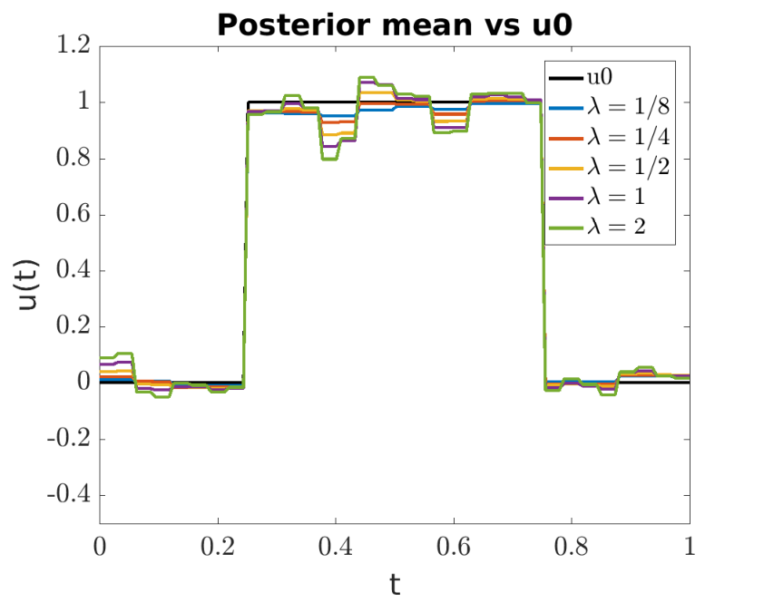
In Figure 11(b) we show the posterior mean for different choices of $N$ . The mean appears to converge as $N$ increases and is able to find the discontinuities in the original function and match their height. The mean is less regular as compared to the true solution $u_{0}$ , most likely due to noise in the data $y$ .

In Figure 11(c) we show a few independent samples from the posterior in the case when $N=128$ . The samples were chosen to be far enough apart that they can be regarded as independent according to the estimated ESS of the worst performing component of the chain. We note that the posterior samples also have the correct location of the discontinuities.

Figure 12 shows the posterior mean and standard deviation of the first eight wavelet coefficients of the Markov chain (i.e., $\{\gamma_{k}\eta_{k}\}_{k=1}^{8}$ ). We observe that the posterior mean is a close match to the true value of the wavelet coefficients of $u_{0}$ which reaffirms our initial observation that the posterior mean is a good predictor of $u_{0}$ . An interesting observation is that posterior standard deviations of the wavelet modes were consistent across different modes. Indicating that, at least the first few modes of $u_{0}$ are approximated with more or less the same uncertainty.

Finally, Figure 13 shows two-dimensional histograms of the first five wavelet modes of $u$ . In comparing the fifth wavelet coefficient $u_{5}$ against $u_{1}$ to $u_{4}$ (i.e, the last row in Figure 13) we observe some concentration of the posterior mass around $u_{5}=0$ .

a) b) c)

Figure 11: a) True function

u_{0}

, its convolved version with kernel width

\varepsilon=1/16

and the noisy pointwise measurements

y

in the deconvolution problem of Example 7. b) The posterior mean of the deconvolution problem for different values of

N

(the number of wavelet coefficients). c) A few posterior samples in the deconvolution example with

N=128

. The samples were taken to be far enough from each other that they can be considered as independent according to the ACF of the worst performing component of the chain.

Figure 12: Posterior mean and standard deviation of the first eight wavelet coefficients in the deconvolution problem with

p=2/3,\lambda=1

and for different values of

N

5.3.2 Algorithm performance

We now turn our attention to the performance of the lifted RCAR algorithm. In Figure 14(a) we show statistics on the ESS of the different components of the Markov chain. Based on these results, in the case where $N=128$ , an independent sample was obtained roughly every $500$ steps. While the ESS deteriorated initially; as $N$ becomes larger the ESS values appeared to settle down for all components. The minimum, mean and the maximum ESS values did not change significantly for $N\geq 16$ .

Since the lifted RCAR algorithm is reversible in infinite dimensions we expect the acceptance ratio to remain bounded away from zero as $N$ becomes large. In Figure 14(b) we plot the average acceptance ratio of lifted RCAR for different values of $\beta$ . As before we fixed $p=2/3$ and $\lambda=1$ . We used a burnin of $5\times 10^{4}$ steps and computed the average acceptance rates over $2\times 10^{5}$ steps with five restarts and averaged the acceptance ratios over the five trials. The acceptance ratios remained more or less consistent as a function of $N$ which is in line with the reversibility of the infinite-dimensional limit of the algorithm.

5.3.3 Effect of hyperparameters $p$ and $\lambda$

We now study the effect of the hyperparameters $p$ and $\lambda$ on the posterior as well as performance of the lifted RCAR algorithm. In all of the examples below we fixed $N=32$ and $\beta=0.97$ .

First, we considered different values of $p=1,4/5,3/5,2/5,1/5$ . Figure 15 depicts the posterior mean and standard deviation of the first eight wavelet modes of the Markov chain for different $p$ . In Figure 15(a) we observe that for all values of $p$ the posterior mean was consistent and varied only slightly. While the posterior mean appeared to be insensitive to choice of $p$ the posterior standard deviation seems to be quite sensitive to $p$ . This is evident in Figure 15(b) where the standard deviation of the higher modes reduced with $p$ .

Next, we considered the effect of $p$ on RCAR’s performance. Figure 16(b) shows that the ESS dropped when $p$ was too small or too big. We also see that for fixed $\beta$ the acceptance ratio dropped when $p$ becomes larger. Similarly, the acceptance ratio increased as $p$ was reduced. Overall, we conclude that the optimal choice of the step size $\beta$ is sensitive to the choice of $p$ .

Figure 15: Posterior mean and standard deviation of the first eight wavelet modes in the deconvolution problem for different values of the parameter

p

Finally we consider the $\lambda$ parameter. We fixed $p=2/3$ and varied $\lambda$ between $1/4$ and $4$ . Recall that $\lambda$ controls the global variance of the wavelet modes of the solution. Figure 18(a) shows empirical posterior mean and standard deviation of the first eight wavelet modes for different values of $\lambda$ . The posterior mean was somewhat sensitive to the choice of $\lambda$ specially for the higher wavelet modes. This sensitivity to $\lambda$ is evident in Figure 17(a) where the posterior mean seems to have higher variation for larger $\lambda$ . We can also see the effect of $\lambda$ in the posterior standard deviations. Figure 18(b) shows that increasing $\lambda$ resulted in increased posterior variance which is expected considering that posterior variance is closely related to that of the prior and the measurement noise. Finally, in Figure 17(b) we present the average acceptance ratio and ESS of the Markov chains for different values of $\lambda$ . All of these simulations shared the same value of $\beta=0.97$ . We observe that both the average acceptance ratio and ESS dropped as $\lambda$ was increased.

Figure 18: Posterior mean and standard deviation of the first eight wavelet modes in the deconvolution problem for different values of the parameter

\lambda

5.3.4 Effect of kernel width $\varepsilon$ and correlations in the data

For our final set of experiments we considered the effect of the kernel width $\varepsilon$ on the quality of the posterior mean as a pointwise approximation to $u_{0}$ . Intuitively, larger values of $\varepsilon$ result in more smoothing that in turn results in more correlated measurements and overall less information in the data as evident in Figure 19. Throughout these experiments we used $N=32$ and $\beta=0.97$ . In Figure 20(a) we show the posterior means for different $\varepsilon$ and compare them to $u_{0}$ . We observe more deviation from $u_{0}$ for larger values of $\varepsilon$ which is expected following our intuition that $y$ is less informative when the forward map is more smoothing. This is also evident in the average acceptance ratios reported in Figure 20(b). Since $y$ was less informative for larger $\varepsilon$ , the posterior was more dominated by the prior rather than the likelihood. Since the lifted RCAR algorithm is prior reversible we expect it to perform better with larger $\varepsilon$ . More evidence of this phenomenon can be seen in Figure 21(b) where larger values of $\varepsilon$ resulted in larger posterior uncertainty in the wavelet modes indicating that the likelihood is less dominant. We highlight that regardless of the effect of $\varepsilon$ on the posterior uncertainties the posterior mean remained a qualitatively good approximator of $u_{0}$ .

Figure 19: True function

u_{0}

along with its convolved version with various kernel widths

\varepsilon=1/16,1/8,1/4

and a realization of the noisy pointwise measurements

y

for each kernel width. Larger values of

\varepsilon

result in more smoothing which in turn results in more correlation in

y

a) b) $\varepsilon$ $\min$ ESS mean ESS $\max$ ESS mean $a(\cdot,\cdot)$ 1/16 15 43 123 0.27 1/8 30 48 102 0.31 1/4 24 47 87 0.37

Figure 20: a) Posterior mean of the deconvolution problem of Example 7 for different choices of the kernel width

\varepsilon

. We observe more deviation from the true solution

u_{0}

for larger values of

\varepsilon

. b) Certain statistics on the ESS of the components of the Markov chain for different values of

\varepsilon

as well as the average acceptance ratio computed over

5\times 10^{5}

samples. All simulations are performed with

N=32

and

\beta=0.97

Figure 21: Posterior mean and standard deviation of the first eight wavelet modes in the deconvolution problem of Example 7 for different values of the kernel width

\varepsilon

. Posterior standard deviations appear to grow with

\varepsilon

. This is in line with the intuition that more smoothing in the forward map results in more uncertainty in the posterior due to less information in the data

y

6 Closing remarks

In the beginning of this article we set out to design algorithms for sampling measures $\nu$ that are absolutely continuous with respect to an underlying non-Gaussian prior measure $\mu$ . We focused on the class of MH algorithms that utilize $\mu$ -reversible proposal kernels and showed that such MH algorithms are reversible with respect to $\nu$ under mild conditions. We then introduced two classes of algorithms called RCAR and SARSD that use autoregressive type proposals that are $\mu$ -reversible for certain priors $\mu$ . The RCAR algorithm is applicable to gamma-type distributions while SARSD can be applied when $\mu$ is SD. While SARSD is in principle more widely applicable, it is often difficult to implement due to issues with computing the time-reversal of AR(1) proposal kernels.

Afterwards we introduced the Bessel-K priors as a concrete example of a non-Gaussian prior for which the RCAR and SARSD algorithms are applicable. We further motivated the Bessel-K priors as interesting candidates for modelling sparse or compressible parameters. We then derived different versions of RCAR and SARSD for the Bessel-K priors on Hilbert spaces and studied the performance of both algorithms in various numerical examples.

6.1 Future directions and open problems

Our exposition is a step towards the design of MCMC algorithms that are tailored to highly non-Gaussian priors. Our overall approach is that by analyzing the prior measure one can design proposals that result in well-defined and efficient algorithms in general state spaces. This is in contrast with existing approaches in the literature [9, 41] that often introduce a non-linear mapping that transforms the prior to a Gaussian or another well-known measure and modify the forward map or the likelihood to allow for application of conventional sampling algorithms with Gaussian priors. Our approach gives rise to many interesting questions that, to the knowledge of the author, have not been addressed in the literature.

The first question is whether our approach can be extended to larger classes of prior measures. That is, whether it is possible to design RCAR or SARSD algorithms for priors that belong to larger classes than the SD class or generalizations of the gamma distribution. Good candidates here are the classes of infinitely-divisible or convex priors that were discussed in [15, 14] or the stable priors of [35]. Another good candidate is limit distributions of random coefficient autoregressive processes that are time-reversible.

Another promising avenue of research is the design of likelihood aware proposal kernels for non-Gaussian priors in contrast with the prior preserving kernels of this work. The RCAR and SARSD algorithms perform well when the likelihood is not dominant and the posterior is close to the prior. Intuitively, this is due to the fact that the proposal kernel of RCAR and SARSD depends only on the prior and not the likelihood. Then a natural question is whether information regarding the gradient of the likelihood can be incorporated into the proposals to construct more efficient algorithms similarly to MALA or HMC.

Finally, we note that the design and implementation of the SARSD algorithm relies on identifying the innovation of the underlying SD prior and the associated reverse kernel of the forward AR(1) proposal. A large portion of the existing literature on SD measures focuses on identifying the innovation measures and so a lot can be said about the forward kernel of SARSD. However, results on the reverse kernels are scarce and this is the main hurdle in implementing SARSD with most SD prior measures besides the exponential distribution and its extensions.

Acknowledgements

The author is thankful to Profs. Derek Bingham, David Campbell, Nilima Nigam and Andrew M. Stuart as well as Dr. James E. Johndrow and Sam Powers for interesting discussions and comments. We also owe a debt of gratitude to the anonymous reviewers whose careful comments and questions helped us improve an earlier version of this article. The author is also supported by a PDF fellowship granted by the Natural Sciences and Engineering Research Council of Canada.

References

[1] Rice wavelet toolbox (rwt) version 3.0. https://github.com/ricedsp/rwt.
[2] O. E. Barndorff-Nielsen, J. Pedersen, and K.-I. Sato. Multivariate subordination, self-decomposability and stability. Advances in Applied Probability, 33(01):160–187, 2001.
[3] O. E. Barndorff-Nielsen and S. Thorbjørnsen. Self-decomposability and Lévy processes in free probability. Bernoulli, 8(3):323–366, 2002.
[4] A. Beskos, M. Girolami, S. Lan, P. E. Farrell, and A. M. Stuart. Geometric MCMC for infinite-dimensional inverse problems. Journal of Computational Physics, 335:327–351, 2017.
[5] A. Bhattacharya, D. Pati, N. S. Pillai, and D. B. Dunson. Dirichlet–Laplace priors for optimal shrinkage. Journal of the American Statistical Association, 110(512):1479–1490, 2015.
[6] V. I. Bogachev. Gaussian Measures, volume 62 of Mathematical Surveys and Monographs. American Mathematical Society, Providence, 1998.
[7] V. I. Bogachev. Measure Theory, volume 1. Springer, New York, 2007.
[8] D. Calvetti and E. Somersalo. An Introduction to Bayesian Scientific Computing: Ten Lectures on Subjective Computing, volume 2 of Surveys and Tutorials in the Applied Mathematical Sciences. Springer Science & Business Media, New York, 2007.
[9] V. Chen, M. M. Dunlop, O. Papaspiliopoulos, and A. M. Stuart. Robust MCMC sampling with non-Gaussian and hierarchical priors in high dimensions. arXiv preprint: 1803.03344, 2018.
[10] S. L. Cotter, G. O. Roberts, A. M. Stuart, and D. White. MCMC methods for functions: modifying old algorithms to make them faster. Statistical Science, 28(3):424–446, 2013.
[11] T. Cui, K. J. Law, and Y. M. Marzouk. Dimension-independent likelihood-informed MCMC. Journal of Computational Physics, 304:109–137, 2016.
[12] M. Dashti, S. Harris, and A. M. Stuart. Besov priors for Bayesian inverse problems. Inverse Problems and Imaging, 6(2):183–200, 2012.
[13] M. Dashti and A. M. Stuart. The Bayesian approach to inverse problems. In R. Ghanem, D. Higdon, and H. Owhadi, editors, Handbook of Uncertainty Quantification, pages 1–118. Springer International Publishing, 2016.
[14] B. Hosseini. Well-posed bayesian inverse problems with infinitely divisible and heavy-tailed prior measures. SIAM/ASA Journal on Uncertainty Quantification, 5:1024–1060, 2017.
[15] B. Hosseini and N. Nigam. Well-posed Bayesian inverse problems: priors with exponential tails. SIAM/ASA Journal on Uncertainty Quantification, 5:436–465, 2017.
[16] N. L. Johnson, S. Kotz, and N. Balakrishnan. Continuous Univariate Distributions, Volume 1, Models and Applications. John Wiley & Sons, New York, second edition, 2002.
[17] Z. J. Jurek. Different aspects of self-decomposability. In O. E. Barndorff-Nielsen, editor, Lévy Processes: theory and applications, pages 367–377. Center for Mathematical Physics and Stochastics.
[18] Z. J. Jurek. Self-decomposability: an exception or a rule. Annales Universitatis Marie Curie-Sklodowska Lublin-Polonia, Section A, 10:93–107, 1997.
[19] Z. J. Jurek and W. Vervaat. An integral representation for self-decomposable Banach space valued random variables. Probability Theory and Related Fields, 62(2):247–262, 1983.
[20] J. Kaipio and E. Somersalo. Statistical and Computational Inverse Problems, volume 160 of Applied Mathematical Sciences. Springer Sience & Business Media, New York, 2005.
[21] S. Kotz, T. J. Kozubowski, and K. Podgorski. The Laplace distribution and generalizations: a revisit with applications to communications, economics, engineering, and finance. Springer Science & Business Media, New York, 2012.
[22] A. Kumar and B. Schreiber. Self-decomposable probability measures on Banach spaces. Studia Mathematica, 53(1):55–71, 1975.
[23] M. Lassas, E. Saksman, and S. Siltanen. Discretization-invariant Bayesian inversion and Besov space priors. Inverse Problems and Imaging, 3(1):87–122, 2009.
[24] A. Lawrance. The innovation distribution of a gamma distributed autoregressive process. Scandinavian Journal of Statistics, pages 234–236, 1982.
[25] P. A. Lewis, E. McKenzie, and D. K. Hugus. Gamma processes. Stochastic Models, 5(1):1–30, 1989.
[26] F. Lucka. Fast Markov chain Monte Carlo sampling for sparse Bayesian inference in high-dimensional inverse problems using L1-type priors. Inverse Problems, 28(12):125012, 2012.
[27] F. Lucka. Fast Gibbs sampling for high-dimensional Bayesian inversion. Inverse Problems, 32(11):115019, 2016.
[28] A. M. Mathai. On noncentral generalized Laplacianness of quadratic forms in normal variables. Journal of multivariate analysis, 45(2):239–246, 1993.
[29] D. F. Nicholls and B. G. Quinn. Random Coefficient Autoregressive Models: An Introduction: An Introduction, volume 11 of Lecture Notes in Statistics. Springer Science & Business Media, New York, 2012.
[30] R. A. Norton and C. Fox. Tuning of MCMC with Langevin, Hamiltonian, and other stochastic autoregressive proposals. arXiv preprint 1610.00781, 2016.
[31] M. Ottobre, N. S. Pillai, F. J. Pinski, A. M. Stuart, et al. A function space HMC algorithm with second order Langevin diffusion limit. Bernoulli, 22(1):60–106, 2016.
[32] K. Pearson, G. Jeffery, and E. M. Elderton. On the distribution of the first product moment-coefficient, in samples drawn from an indefinitely large normal population. Biometrika, pages 164–201, 1929.
[33] F. W. Steutel and K. Van Harn. Infinite divisibility of probability distributions on the real line. Pure and Applied Mathematics. Marcel Dekker Inc., New York, 2003.
[34] A. M. Stuart. Inverse problems: a Bayesian perspective. Acta Numerica, 19:451–559, 2010.
[35] T. Sullivan. Well-posed bayesian inverse problems and heavy-tailed stable quasi-banach space priors. Inverse Problems & Imaging, 11(5):857–874, 2017.
[36] D. H. Thang. Random mappings on infinite dimensional spaces. Stochastics: An International Journal of Probability and Stochastic Processes, 64(1-2):51–73, 1998.
[37] L. Tierney. A note on Metropolis-Hastings kernels for general state spaces. Annals of Applied Probability, 8(1):1–9, 1998.
[38] K. Urbanik. Self-decomposable probability distributions on ${\mathbb{R}}^{m}$ . Applicationes Mathematicae, 10(1):91–97, 1969.
[39] C. R. Vogel. Computational Methods for Inverse Problems. SIAM, Philadelphia, 2002.
[40] S. G. Walker. A note on the innovation distribution of a gamma distributed autoregressive process. Scandinavian journal of statistics, 27(3):575–576, 2000.
[41] Z. Wang, J. M. Bardsley, A. Solonen, T. Cui, and Y. M. Marzouk. Bayesian inverse problems with l_1 priors: A randomize-then-optimize approach. SIAM Journal on Scientific Computing, 39(5):S140–S166, 2017.
[42] G. Weiss. Time-reversibility of linear stochastic processes. Journal of Applied Probability, 12(4):831–836, 1975.

Appendix

A Self-decomposable measures

We say $\mu\in P(X)$ is SD if for every choice of $\beta$ there exists a $\mu_{\beta}\in P(X)$ so that [22]

\widehat{\mu}(\varrho)=\widehat{\mu}(\beta\varrho)\widehat{\mu}_{\beta}(\varrho)\qquad\forall\varrho\in X^{\ast}.

(36)

Here $\widehat{\mu}$ is the characteristic function of $\mu$ and $X^{\ast}$ is the dual of $X$ . The measure $\mu_{\beta}$ is referred to as the innovation of $\mu$ . In other words, a random variable $\xi$ is SD if, for every $\beta\in(0,1)$ there exists an independent random variable $\xi_{\beta}$ so that the law of $\xi_{\beta}$ coincides with the law of $\beta\xi+\xi_{\beta}$ . The SD random variables are a subclass of infinitely-divisible random variables [33] that were first introduced by Paul Lévy (the SD class is also known as the class of Lévy L probability measures). The SD class includes well-known probability measures such as Gaussian measures and certain generalizations of the Laplace and gamma distributions. For the most part, the theory of SD measures was developed in the 1960s in connection to the theory of Lévy processes. A detailed study of the SD class can be found in the works of Kumar and Schreiber [22] and Urbanik [38] as well as Jurek [18, 17, 19] and Barndorff-Nielsen [2, 3]. We refer the reader to [33, Ch. V] for an accessible introduction to real valued SD random variables.

B Some random variables on the real line

Here we gather the definition of some standard random variables that are used throughout the article in order to specify the parameterizations used in our article.

Definition B.1 (Gamma random variable).

A positive random variable $\xi$ is distributed according to a gamma distribution $G(p,\sigma)$ with shape parameter $p>0$ and scale parameter $\sigma>0$ if its law has Lebesgue density

{\rm Gamm}(p,\sigma;t)=\frac{1}{\sigma\Gamma(p)}\left(\frac{t}{\sigma}\right)^{p-1}\exp\left(-\frac{t}{\sigma}\right)\mathbf{1}_{(0,\infty)}(t)\qquad\text{for}\qquad t\in\mathbb{R}.

(37)

Definition B.2 (Exponential random variable).

A positive random variable $\xi$ is distributed according to a exponential distribution ${\rm Exp}(\sigma)$ with parameter $\sigma>0$ if its law has Lebesgue density

{\rm Exp}(\sigma;t)=\frac{1}{\sigma}\exp\left(-\frac{t}{\sigma}\right)\mathbf{1}_{(0,\infty)}(t)\qquad\text{for}\qquad t\in\mathbb{R}.

(38)

Definition B.3 (Laplace random variable).

A real valued random variable $\xi$ is distributed according to a Laplace distribution ${\rm Lap}(\sigma)$ with parameter $\sigma>0$ if its law has Lebesgue density

{\rm Lap}(\sigma;t)=\frac{1}{2\sigma}\exp\left(-\left|\frac{t}{\sigma}\right|\right)\text{for}\qquad t\in\mathbb{R}.

(39)

Definition B.4 (Beta random variable).

A random variable $\xi\in(0,1)$ is distributed according to a beta distribution ${\rm Beta}(p,q)$ with parameters $p,q>0$ if its law has Lebesgue density

{\rm Beta}(p,q;t)=\frac{\Gamma(p+q)}{\Gamma(p)\Gamma(q)}t^{p-1}(1-t)^{q-1}\mathbf{1}_{(0,1)}(t)\qquad\text{for}\qquad t\in\mathbb{R}.

(40)

Definition B.5 (Bernoulli random variable).

A random variable $\xi\in\{0,1\}$ is distributed according to a Bernoulli distribution ${\rm Bern}(p)$ with parameter $p\in(0,1)$ if

\mathbb{P}(\xi=0)=1-p,\qquad\mathbb{P}(\xi=1)=p.

(41)

Definition B.6 (Poisson random variable).

A random variable $\xi\in\mathbb{N}$ is distributed according to a Poisson distribution ${\rm Pois}(c)$ with rate $c>0$ if

\mathbb{P}(\xi=k)=\frac{c^{k}\exp(-c)}{k!},\qquad\forall k\in\mathbb{N}.

C Properties of gamma and exponential random variables

Here we collect some results on exponential and gamma distributions that are used in the design of the RCAR and SARSD algorithm for 1D Bessel-K priors in Section 3.

C.1 Properties of the gamma distribution

Observe that ${\rm Gamm}(1,\sigma)$ coincides with the law of an exponential random variable ${\rm Exp}(\sigma)$ . A straightforward calculation shows that the gamma distribution has bounded raw moments of all orders, in fact

\int_{0}^{\infty}t^{k}{\rm Gamm}(p,\sigma;t)\>{\rm d}\Lambda(t)=\frac{\sigma^{k}\Gamma\left({k+p}\right)}{\Gamma(p)}.

(42)

C.1.1 The thinned gamma process

It is well-known [16, Ch. 17.6] that given independent random variables $\xi\sim{\rm Gamm}(p_{1},\sigma)$ and $\xi^{\prime}\sim{\rm Gamm}(p_{2},\sigma)$ then $\xi+\xi^{\prime}\sim{\rm Gamm}(p_{1}+p_{2},\sigma)$ and $\frac{\xi}{\xi+\xi^{\prime}}\sim{\rm Beta}(p_{1},p_{2})$ and furthermore $\xi+\xi^{\prime}$ and $\frac{\xi}{\xi+\xi^{\prime}}$ are independent. In light of this fact we consider an RCAR(1) process of the form

u^{(n)}=\zeta^{(n)}u^{(n-1)}+w^{(n)},\qquad\zeta^{(n)}\stackrel{{\scriptstyle iid}}{{\sim}}{\rm Beta}(p\beta,p(1-\beta)),\quad w^{(n)}\stackrel{{\scriptstyle iid}}{{\sim}}{\rm Gamm}(p(1-\beta),\sigma),\qquad

for fixed parameter $\beta\in(0,1)$ . The limit distribution of this RCAR(1) process is precisely ${\rm Gamm}(p,\sigma)$ [25]. Moreover, this process is time-reversible and so the transition kernel

\mathcal{Q}(u,\>{\rm d}v)={\rm Law}\{v=\zeta u+w,\qquad\zeta\sim{\rm Beta}(p\beta,p(1-\beta)),w\sim{\rm Gamm}(p(1-\beta),\sigma)\},

(43)

satisfies detailed balance with respect to ${\rm Gamm}(p,\sigma)$ .

C.1.2 Self-decomposability

The gamma distribution is SD. We demonstrate this using the characteristic function of ${\rm Gamm}(p,\sigma)$ . Recall

\widehat{{\rm Gamm}}(p,\sigma;s)=(1-is\sigma)^{-p}.

(44)

Choose $\beta\in(0,1)$ and define

\widehat{{\rm Gamm}}_{\beta}(p,\sigma;s):=\frac{\widehat{{\rm Gamm}}(p,\sigma;s)}{\widehat{{\rm Gamm}}(p,\sigma;\beta s)}=\left(\frac{1-i\beta s\sigma}{1-is\sigma}\right)^{p}=\left(\beta+\frac{1-\beta}{1-is\sigma}\right)^{p}.

(45)

It is straightforward to check that

\widehat{{\rm Gamm}}(p,\sigma;s)=\widehat{{\rm Gamm}}(p,\sigma;\beta s)\widehat{{\rm Gamm}}_{\beta}(p,\sigma;s).

But $\widehat{{\rm Gamm}}(p,\sigma;\beta s)$ is simply the characteristic function of $\beta\xi$ . Furthermore, $\widehat{{\rm Gamm}}_{\beta}(p,\sigma;0)=1$ and $|\widehat{{\rm Gamm}}_{\beta}(p,\sigma;s)|\leq 1$ . In fact, $\widehat{{\rm Gamm}}_{\beta}$ is continuous and differentiable at 0 and so it is the characteristic function of a random variable on $\mathbb{R}$ . We denote this variable by $\xi_{\beta}$ and its law by ${{\rm Gamm}}_{\beta}(p,\sigma)$ . On this account, we have the following decomposition of gamma random variables:

\xi\stackrel{{\scriptstyle d}}{{=}}\beta\xi^{\prime}+\xi_{\beta},

(46)

where $\xi,\xi^{\prime}\sim{\rm Gamm}(p,\sigma)$ and $\xi_{\beta}\sim{\rm Gamm}_{\beta}(p,\sigma)$ are independent of each other. Lawrance [24] showed that $\xi_{\beta}$ is a compound Poisson random variable of the form

\xi_{\beta}\stackrel{{\scriptstyle d}}{{=}}\sum_{k=1}^{\tau}\beta^{\eta_{k}}\theta_{k}\qquad\text{where}\qquad\tau\sim\text{Pois}(p\log(1/\beta)),\quad\eta_{k}\sim U(0,1),\quad\theta_{k}\sim{\rm Exp}(\sigma),

(47)

where $\tau$ , $\eta_{k}$ and $\theta_{k}$ are all independent and the latter sequences are identically distributed and $U(0,1)$ denotes the uniform distribution on $[0,1]$ . Note that with the above expression we can simulate $\xi_{\beta}$ exactly. This is not possible for general SD random variables. We also note that a more efficient recipe for simulating $\xi_{\beta}$ was discovered by Walker [40].

C.2 Self-decomposability of the exponential distribution

Using the fact that ${\rm Exp}(\sigma)={\rm Gamm}(1,\sigma)$ we have that the characteristic function of an ${\rm Exp}(\sigma)$ random variable is given by

\widehat{{\rm Exp}}(\sigma;s)=(1-is\sigma)^{-1}.

Using the factorization

\frac{1}{1-is}=\left(\frac{1}{1-i\beta s}\right)\left(\beta+\frac{1-\beta}{1-it}\right)

for $\beta\in(0,1)$ we infer that ${\rm Exp}(1)$ is SD and

{\rm Exp}_{\beta}(1)={\rm Law}\{\zeta w,\qquad\zeta\sim{\rm Bern}(1-\beta),w\sim{\rm Exp}(1)\}.

We can then easily extend this to other exponential distributions to get

{\rm Exp}_{\beta}(\sigma)={\rm Law}\{\zeta w,\qquad\zeta\sim{\rm Bern}(1-\beta),w\sim{\rm Exp}(\sigma)\}.

(48)

Thus the transition kernel

\mathcal{Q}(u,\>{\rm d}v)={\rm Law}\{v=\beta u+\zeta w,\qquad\zeta\sim{\rm Bern}(1-\beta),w\sim{\rm Exp}(\sigma)\}

(49)

preserves the distribution ${\rm Exp}(\sigma)$ but it does not satisfy detailed balance. However, we can directly compute the reverse kernel $\mathcal{Q}^{\ast}$ . Consider, $u,w\stackrel{{\scriptstyle iid}}{{\sim}}{\rm Exp}(1)$ and $\zeta\sim{\rm Bern}(1-\beta)$ then

v=\beta u+\zeta w,

and $v\sim{\rm Exp}(1)$ . We wish to find an expression for $u|v$ but this is not trivial since $v$ is not independent of $\zeta$ and $w$ . Let $f(v|u)$ denote the distribution of $v$ given $u$ , i.e.,

f(v|u)=\beta\delta_{\beta u}(v)+(1-\beta)\exp(-(t-\beta u))\mathbf{1}_{[\beta u,\infty)}(v).

Using Bayes’ rule we now have for $v>0$

	$\displaystyle f(u\|v)$	$\displaystyle=\frac{f(v\|u)f(u)}{f(v)}$
		$\displaystyle=\frac{1}{\exp(-v)}\left(\beta\delta_{\beta u}(v)+(1-\beta)\exp(-(v-\beta u))\mathbf{1}_{[\beta u,\infty)}(v)\right)\exp(-u)\mathbf{1}_{[0,\infty)}(u)\>{\rm d}u$
		$\displaystyle=\beta\delta_{\beta u}(v)\exp(-u+v)\>{\rm d}u+(1-\beta)\exp(-(1-\beta)u)\mathbf{1}_{[\beta u,\infty)}(v)\mathbf{1}_{[0,\infty)}(u)\>{\rm d}u$
		$\displaystyle=\beta\delta_{v/\beta}(u)\exp\left(-\frac{1-\beta}{\beta}v\right)\>{\rm d}u+(1-\beta)\exp(-(1-\beta)u)\mathbf{1}_{[\beta u,\infty)}(v)\mathbf{1}_{[0,\infty)}(u)\>{\rm d}u$
		$\displaystyle=\frac{\beta}{1-\beta}\delta_{v/\beta}\left(\frac{\zeta}{1-\beta}\right)\exp\left(-\frac{1-\beta}{\beta}\right)\>{\rm d}\zeta+\mathbf{1}_{[0,v/\beta]}\left(\frac{\zeta}{1-\beta}\right)\exp(-\zeta)\>{\rm d}\zeta$
		$\displaystyle=\mathbb{P}\left(\frac{\zeta}{1-\beta}\geq\frac{v}{\beta}\right)\delta_{v/\beta}\left(\frac{\zeta}{1-\beta}\right)+\mathbf{1}_{[0,v/\beta]}\left(\frac{\zeta}{1-\beta}\right)\exp(-\zeta)\>{\rm d}\zeta$

where we used the change of variables $\zeta=(1-\beta)u$ . We now observe that the above expression is precisely the law of $\min\{v/\beta,\zeta/(1-\beta)\}$ where $\zeta\sim{\rm Exp}(1)$ . Thus the reverse kernel $\mathcal{Q}^{\ast}$ associated to (49) can be identified as

\mathcal{Q}^{\ast}(v,\>{\rm d}u)={\rm Law}\left\{u=\min\{v/\beta,\zeta/(1-\beta)\},\qquad\zeta\sim{\rm Exp}(1)\right\}.

(50)

Two Metropolis-Hastings algorithms for posterior measures with non-Gaussian priors in infinite dimensions

Abstract

Keywords:

MSC

1 Introduction

1.1 Some notation and definitions

2 Metropolis-Hastings algorithms with prior reversible proposals

2.1 Prior-reversible proposal kernels

Theorem 2.1.

2.2 The RCAR algorithm

Example 1.

Example 2.

2.3 The SARSD algorithm

Example 3.

3 The Bessel-K prior

Example 4.

3.1 From gamma to Bessel-K distributions

Definition 3.1 (Bessel-K distribution).

3.2 Sampling with Bessel-K priors in 1D

3.2.1 The lifted RCAR algorithm

3.2.2 The lifted SARSD algorithm for integer pp

Remark 3.1.

Remark 3.2.

3.3 Generalization to infinite dimensions

Theorem 3.1 ([14, Thm. 2.3 and 2.4]).

Definition 3.2 (B​K​(p,ℛ)BK(p,\mathcal{R}) prior).

Theorem 3.2.

Theorem 3.3.

Proof.

3.3.1 Connection to Besov priors

Definition 3.3 (Bq​qs​(𝕋d)B^{s}_{qq}(\mathbb{T}^{d}) prior).

3.4 Sampling with Bessel-K priors on Hilbert spaces

Theorem 3.4.

Proof.

3.4.1 The lifted RCAR and SARSD algorithms on Hilbert spaces

Remark 3.3.

Remark 3.4.

4 Well-posed Bayesian inverse problems with Bessel-K priors

Definition 4.1 (Hellinger Well-posedness [15]).

Theorem 4.1.

Corollary 4.1.

Theorem 4.2.

Corollary 4.2.

5 Numerical experiments

5.1 Example 5: Density estimation for a linear inverse problem in 2D

5.2 Example 6: Denoising in finite dimensions with a gamma prior

5.3 Example 7: Deconvolution on the circle with Bessel-K priors

5.3.1 Posterior statistics

5.3.2 Algorithm performance

5.3.3 Effect of hyperparameters pp and λ\lambda

5.3.4 Effect of kernel width ε\varepsilon and correlations in the data

6 Closing remarks

6.1 Future directions and open problems

Acknowledgements

References

References

Appendix

A Self-decomposable measures

B Some random variables on the real line

Definition B.1 (Gamma random variable).

Definition B.2 (Exponential random variable).

Definition B.3 (Laplace random variable).

Definition B.4 (Beta random variable).

Definition B.5 (Bernoulli random variable).

Definition B.6 (Poisson random variable).

C Properties of gamma and exponential random variables

C.1 Properties of the gamma distribution

C.1.1 The thinned gamma process

C.1.2 Self-decomposability

C.2 Self-decomposability of the exponential distribution

3.2.2 The lifted SARSD algorithm for integer $p$

Definition 3.2 ( $BK(p,\mathcal{R})$ prior).

Definition 3.3 ( $B^{s}_{qq}(\mathbb{T}^{d})$ prior).

5.3.3 Effect of hyperparameters $p$ and $\lambda$

5.3.4 Effect of kernel width $\varepsilon$ and correlations in the data