Solid-state magnetic traps and lattices
Abstract
We propose and analyze magnetic traps and lattices for electrons in semiconductors. We provide a general theoretical framework and show that thermally stable traps can be generated by magnetically driving the particle’s internal spin transition, akin to optical dipole traps for ultra-cold atoms. Next we discuss in detail periodic arrays of magnetic traps, i.e. magnetic lattices, as a platform for quantum simulation of exotic Hubbard models, with lattice parameters that can be tuned in real time. Our scheme can be readily implemented in state-of-the-art experiments, as we particularize for two specific setups, one based on a superconducting circuit and another one based on surface acoustic waves.
I Introduction
The advent of cold atoms trapped in optically defined potential landscapes has enabled experimental breakthroughs in various discplines ranging from condensed-matter physics to quantum information processing [1, 2]. Especially, thanks to largely tunable system parameters and the possibility to mimic and gain understanding of complex solid-state systems, ultra-cold atomic gases have become a rich playground and valuable tool to explore novel quantum many-body physics [3]. On a complementary route towards controllabe quantum matter and a fully fledged quantum simulator, solid-state platforms allow to pursue the same goals in a very different physical context, both bearing challenges such as to overcome impurity-induced disorder in semiconductor systems [4], but also offering the potential to benefit from long-range inter-particle interactions, access to a wide variety of quasiparticles and, in principle, means to build scalable on-chip architectures for quantum information processing. To this end, different kinds of quasiparticle traps in semiconductor nanostructures have been proposed and realized [5, 6, 7, 8, 9, 10, 11]. Likewise, in the realm of atomic [12, 13] and molecular [14, 15] systems, mesoscopic on-chip platforms have been tailored to miniaturize experiments with ultracold quantum matter. Apart from more established solid-state platforms like, e.g., quantum-dot based architectures [16], it has recently been proposed [17] to employ surface acoustic waves (SAWs) to trap and control semiconductor quasiparticles such as electrons in intrinsically scalable and tunable acoustic lattices. The latter operate at elevated energy scales with typical lattice spacings nm and recoil energies (where with an effective particle mass which is typically of the order of the electron rest mass) as compared with optical lattices where typically [18]. Inspired by these results and recent advances in the rapidly evolving field of nanomagnetism [19, 20], i.e., the generation and control of (high-frequency) magnetic fields on the nanoscale, the present work aims to bring the favourable scaling properties and flexibility of optical lattices to the solid-state domain.
In contrast to electrically defined confinement potentials for charged particles in quantum wells, the spin degree of freedom (DOF) can be addressed with magnetic field gradients in order to trap and control particles in semiconductor nanostructures; note that this is in close analogy to the working principle of optical dipole traps where the induced AC Stark shift of the atomic levels gives rise to a dipole potential for the atom [21]. In previous theoretical proposals [22, 23] and experimental demonstrations [24, 25], magnetic traps for charge carriers in low-dimensional quantum wells were induced by a spatially inhomogeneous giant Zeeman splitting in dilute magnetic semiconductors (DMS) [26], which feature extremely large -factors . In particular, microscale magnets [27] and current loops [28] as well as superconducting (SC) vortex lattices [23] have been considered in this context. So far, however, none of these previous results have yet been tailored to scalable architectures and, moreover, only static traps with limited tunability of system parameters have been taken into account. In this work, we take a significant next step towards tunable and scalable magnetic lattices and develop a general theoretical framework fit to describe the latter. We show that a non-standard form of the Hubbard model with two independently tunable hopping parameters can readily be implemented. Ultimately, two alternative implementations of the developed model will be discussed in detail, one based on SAWs and the other based on magnetic field gradients generated by SC nanowires, both operated in yet unexplored parameter regimes and with highly favourable tunability and scalability properties.
The basic scheme is depicted in Fig. 1. We consider electrons with two internal (spin) states and which are confined to a conventional low-dimensional quantum well or a purely two-dimensional material, e.g., from the group of transition-metal dichalcogenides (TMDs), and subject to a spatially inhomogeneous magnetic driving field. Due to the thereby induced AC Stark shift acting on the internal energy levels, the electrons feel an effective state-dependent potential which is periodic along one axis (in the one-dimensional setup we consider here), as illustrated in Fig. 1. As a result, the electrons are attracted to a regular lattice of antiferromagnetic character, since the two internal states are found to be trapped at nodes or antinodes of the magnetic field distribution, respectively, cf. Fig. 1(b). For simplicity, we consider only one-dimensional systems, but all results can readily be generalized to two dimensions.
This paper is organized as follows. In Sec. II, we first introduce the theoretical framework to describe magnetic trapping potentials for electrons confined to a two-dimensional electron gas (2DEG). All requirements for the validity of the theoretical treatment and relevant approximations are discussed in Sec. II.1, followed by an investigation of hopping and interactions in magnetic lattices [see Sec. II.2] and a detailed description of possible implementations in Sec. III. Finally, we will provide case studies for both implementations with realistic parameters in Sec. IV.
II General theoretical Framework
II.1 Single-particle physics in magnetic traps
Single-particle physics.—We consider an electron confined to a 2DEG with effective mass and the two internal states and exposed to an external magnetic field, . The spatially homogeneous, static (in-plane) part of the field, , gives rise to a Zeeman splitting, , and the inhomogeneous (time-dependent or time-independent) (out-of-plane) field component, , drives spin transitions with frequency . The corresponding Hamiltonian can be written as (here and in the following, we adopt the convention that )
| (1) |
where , , , denote the particle’s position, momentum and Pauli spin operators, respectively. The inhomogeneous Rabi frequency is denoted by with , where is the gyromagnetic ratio of the electron. We assume in the following, where denotes the wavevector, but more general periodic functions can be considered. While the universality of this model will become more apparent later, especially when we consider different implementations in Sec. III, we may already distinguish between two physically dissimilar cases both captured by Eq. (1): (i) static traps () are time-independent and (ii) dynamic traps () are explicitly time-dependent realizations of the model. Due to their intrinsic flexibility and in-situ tunability of system parameters, we put the main focus on dynamic magnetic traps, i.e., .

Within a co-rotating frame and rotating-wave approximation (RWA) for and , the time-independent internal model can be diagonalized exactly which yields the local eigenenergies with and position-dependent eigenstates,
where . The trap depth of the effective potentials , which is given by the difference , depends only on and and will be denoted by in the following [see Fig. 1]. In the limit , the standard result from second-order perturbation theory, , can be recovered. Note that the periodic modulation of the internal energy levels amounts to a state-dependent potential for the motional DOF such that the states are trapped at nodes and antinodes of the driving field, respectively. As a consequence, magnetic trapping potentials for the two spin components are shifted with respect to one another, as illustrated in Fig. 1(b). In fact, this result is reminiscent of state-dependent optical lattices which can be enriched by laser-assisted tunneling between internal atomic states [29, 30], whereby gauge fields for ultracold atoms can be generated [31, 32, 33, 34].
Note that, in the realm of the RWA introduced before, the Rabi frequency is limited to relatively small values, as compared to other relevant energy scales. This limitation can be overcome, to some extent, by deriving an effective Floquet Hamiltonian without RWA, see Appendix A for details.
Until now, we have not explicitly taken into account the presence of the kinetic term, , in Eq. (1). Its presence induces a coupling between the local spin eigenstates and, as a consequence, undesired spin flips may result in particle loss from the trap [35]. In order to quantify this effect, it is instructive to introduce a unitary transformation which diagonalizes at each point, such that (). The thereby transformed Hamiltonian, , contains the kinetic term from Eq. (1), the diagonal (in the local eigenbasis spanned by and ) spin Hamiltonian and an additional term , which stems from the transformation of the kinetic term, see Appendix B for details. If the latter contributes only a small correction to the system’s characteristic energy scale set by the motional quantum , the internal spin DOF follows adiabatically the local direction of the magnetic field and the contribution from can be safely neglected. For this adiabatic approximation (also refered to as Born-Oppenheimer approximation) to hold, the local eigenstates of the two-level system spanned by and must be sufficiently separated in energy. If this energy gap by far exceeds , i.e. , spin-flip processes are typically negligible [35].
Requirements.—Following the line of arguments outlined above, we have implicitly made a few assumptions about the system parameters which we are going to summarize in the following: (i) We have assumed idealized two-level spin systems with well-resolved energy levels and thus a relatively small intrinsic linewidth . (ii) We require a weak electron-phonon coupling, i.e., the spontaneous phonon emission rate which quantifies motional damping of the electron must be small compared to all other characteristic system’s time scales; explicitly, we demand that it should be smaller than the motional transition frequencies, i.e., . (iii) In order to obtain thermally robust traps and minimize particle loss from the trap, we need thermal energies (where denotes the Boltzmann constant). Typically, in case ground-state cooling is desired, this requirement is replaced by the stronger condition . (With at least one bound state, , supported by the trap, the latter condition is more restrictive.) (iv) The magnetic trap depth is either much smaller than , i.e. in the perturbative regime , or approaches in the opposite limit ; however, in both cases is limited from above by . In terms of other relevant physical parameters contained in , this means that strong magnetic radio-frequency (RF) fields and large g-factors are favourable. (v) The Rabi frequency , in turn, is typically much smaller than the driving frequency within the RWA, , but this condition can be relaxed as mentioned earlier. However, for too large , even the high-frequency expansion of the Floquet Hamiltonian fails to converge. For our purposes, we therefore demand . (vi) Finally, introducing the small number , the adiabaticity condition can be rewritten as . However, this condition may be relaxed at the cost of higher loss rates. The Majorana loss rate , compared to the natural frequency scale of the trap, can be estimated as [35] (compare also Ref. [36] for a related description of non-adiabatic spin-flips in radio-frequency dressed magnetic traps for cold atoms); deep in the adiabatic regime with , spin-flip losses are negligible as , but even for moderate values (), the loss rates are relatively small with (). Hence, the adiabaticity condition may be relaxed in order to obtain well-performing traps. Putting these findings together results in a concise list of necessary requirements and, in general, without resorting to the RWA or the perturbative regime where , we find:
| (2) |
In order to obtain reliable magnetic traps, both implementations discussed in Sec. III need to be operated in a parameter regime where Eq. (2) is fulfilled and is sufficiently small.
II.2 Engineering of Hubbard models
Towards many-body physics.—Based on the theoretical framework fit to describe single traps as worked out above, the following paragraphs are dedicated to the study of Fermi-Hubbard physics in magnetic lattices, i.e., periodic arrays of magnetic traps. Explicitly, we show that spin-dependent forms of the Hubbard model with independently tunable hopping parameters and can be realized with the aid of additional driving fields [see Appendix C for more details] in the fashion of zigzag optical lattices for cold atoms [37, 38]. Here and in the following, denotes spin-conserved next-nearest neighbour coherent tunneling processes and describes spin flip-assisted tunneling between adjacent lattice sites, cf. Fig. 1(b). Another genuine prospect is the operation in a low-temperature, strong-interaction regime (at dilution-fridge temperatures mK) where the thermal energy is much smaller than the hopping parameters which, in turn, are small compared to the on-site interaction strength , i.e., .
As a starting point, we consider the single-particle Hamiltonian within the adiabatic approximation [see Sec. II.1] which can be written as
| (3) |
with . In a next step, we now consider an ensemble of electrons in a magnetic lattice. At sufficiently low temperatures () such that the electrons are confined to the lowest Bloch band, we find that the system is characterized by a Fermi-Hubbard model of the form [39]
| (4) | |||||
where the fermionic operator annihilates (creates) an electron with spin at lattice site , and are the spin-resolved and total occupation numbers, respectively. The summation over is performed for next-nearest neighbours (accordingly, in Eq. (5) denotes a summation over neighbouring sites). quantifies the inter-particle interaction strength ( denotes the on-site interaction strength), where is a Wannier basis function which is typically strongly localized around the respective lattice . Typically, it is inversely proportional to the lattice constant , depends on the dielectric constant of the substrate and can be reduced with the aid of an additional metallic screening layer positioned at a distance from the 2DEG. The screened Coulomb interaction can be written as , where incorporates screening [39, 40]. In Eq. (4) the spin-dependent energy offset [see Fig. 1] incorporates the remnant of the Zeeman splitting (in the rotating frame) and the AC Stark shifts. Moreover, the site-dependent chemical potential can take disorder effects into account [17]. In the tight-binding limit where the potential is sufficiently deep, i.e., (with the recoil energy ), the hopping parameter is approximately given by [3]. Realistic parameter values [see below for details] suggest that the low-temperature, strong-interaction regime eV lies within reach with state-of-the-art experimental techniques.

As illustrated in Fig. 1(b), the standing-wave field distribution, as described by Eq. (1), gives rise to spatially separated traps for the different spin components. Hence, adjacent potential minima host two different spin states and , respectively. As a consequence, spin-flip assisted tunneling between neighbouring lattice sites is strongly suppressed, whereas next-nearest neighbours, occupying the same internal state, are coupled much more strongly via direct tunneling , as captured by Eq. (4). In order to control these hopping matrix elements independently, we consider the application of an additional magnetic driving field at frequency which effectively couples different spin states (at adjacent lattice sites), thus increasing the hopping parameter and at the same time also the ratio . As outlined in Appendix C, this introduces a second hopping term to the Fermi-Hubbard model in Eq. (4) and the resulting Hamiltonian can be written in a suitable co-rotating frame as
| (5) | |||||
where and denote opposite spins (i.e., , or vice versa).
The additional transverse driving field of strength has to be sufficiently small in order to be considered a perturbation to the magnetic-lattice Hamiltonian in Eq. (3); more precisely, we demand . In general, the time-dependence and exact form of this spatially homogeneous field can be derived and reverse-engineered from the desired Hamiltonian in the adiabatic frame, see Appendix C for further details. Since, in the tight-binding regime, next-nearest neighbour hopping is exponentially suppressed, weak driving fields are sufficient to reach situations where and, typically, for moderate driving strengths direct tunneling processes can be safely neglected [29]. In Fig. 2, it is shown how the ratio is affected by sweeping and , while keeping the number of bound states at a constant value. Evidently, smaller driving fields lead to smaller . Moreover, at small (i.e. deep in the perturbative regime, see Sec. II.1), tends to decrease with increasing . By choosing adequate driving fields, the tunneling matrix elements and can thereby be independently tuned over a relatively wide range.
Spin-orbit interaction.—In the presence of strong spin-orbit interaction (SOI), transitions between different spin states at adjacent lattices sites can be induced (eventually, for strong enough SOI, without any external driving field) such that the Hubbard model in Eq. (4) may contain additional SOI-induced hopping terms. Specifically, SOI-induced hopping parameters can be estimated as , where denotes the Rashba and Dresselhaus coupling strengths, respectively. For realistic parameter values, this may give rise to such that nearest and next-nearest neighbour hopping terms become comparable, see Sec. IV for further details. Both the Rashba and Dresselhaus SOI strengths depend on the orientation of the lattice in the host material and can thereby induce anisotropic hopping. This gives access to a wider class of Hubbard models than those captured by Eq. (5).
III Implementations
In the following, we propose two experimental setups for the realization of our model. First, in Sec. III.1, we consider magnetic field gradients provided by a classical current source as an example for a setup which can be operated both in a static (; compare Eq. (1)) or dynamic () mode. Subsequently, we will discuss a purely dynamic (i.e., always ) setup based on surface acoustic waves in Sec. III.2.
III.1 Superconducting circuit
As a first example for a realization of our model as described by Eq. (1), we consider SC circuits operating at GHz frequencies. The electrons are confined in a 2DEG at a distance from a current-carrying wire, which is located above the surface. For our purposes, SC circuits and circuit resonators are attractive because of their capability to generate AC magnetic fields by carrying relatively large currents and the possibility to integrate them in semiconductor nanostructures [42, 43]. In a simple toy model, we describe the circuit by a meandering wire carrying an AC current through parallel sections of the wire separated by a lattice constant , see Fig. 3(a) for an illustration of the setup. Note that, in principle, this setup can also be operated in the static regime () when DC currents and, thus, time-independent fields are considered. The classical electric current density induces a magnetic field which is calculated using the Biot-Savart law, see Fig. 3(b) for an exemplary field distribution as induced by a current source at fixed positions [45].

Here, we consider only one-dimensional trapping potentials in which the electrons are confined to a one-dimensional channel such that the motional DOF is frozen out. Furthermore, we assume that the spatial extension of the meandering wire exceeds the size of the trapping region within the 2DEG, such that finite-size effects of the induced magnetic field can be neglected. This simplifies the mathematical description and we obtain the AC magnetic field distribution for a given wire geometry by summing up the induced fields of all parallel wire segments, see Fig. 3 [for details, cf. Appendix D]. In the presence of an additional static homogeneous field , the resulting Hamiltonian, , approximately coincides with our model in Eq. (1), where we can identify and the amplitude of the Rabi frequency is given by
| (6) |
Eq. (6) becomes exact in the limit of an infinitely long wire and it converges to the numerically exact result in the limit of a long wire and in the center region below the wire [see App. D for further details]; for all practical purposes, it yields sufficiently exact results for typical resonator geometries. The exact spatial pattern of the Rabi frequency depends on both the geometry of the resonator and the ratio . Neglecting finite-size effects and for a perfectly periodic resonator geometry, the Rabi frequency can be approximately written as , see Appendix D for further details.
Let us conclude the description of the proposed setup with a few general remarks. Firstly, we note that the calculation of the Hamiltonian results in an additional time-dependent term which we have neglected here and which is typically very small compared to the time-independent contribution from , see Appendix D for more information. Secondly, the calculated RF field strength mT [see Fig. 3(b)] at a given distance and given current intensity from the surface ranges from realistic to very optimistic values. The highest given values can only be obtained in close proximity to the surface. Moreover, the critical current density MA/cm2 [44] used in our calculations is optimistic because high ( GHz) frequencies and strong ( T) in-plane magnetic fields might reduce this value. However, especially the frequency dependence of is still a current topic of research and, as noted earlier, the proposed setup may also be operated at , i.e., with DC currents. For -factors (e.g., in InAs-based quantum wells), the given range of field strengths amounts to trap depths mK. An explicit case study for specific material parameters follows in Sec. IV, where we check when the requirements set by Eq. (2) can be fulfilled. Finally, we stress that the relevant system parameters from Eq. (2) do not depend on the material choice (except for the -factor of the quantum well) and due to its simplicity, the setup can, in principle, readily be implemented in an experiment. While the trap depth is tunable, the geometry is predefined in this setup, and therefore the lattice constant (thus also the ratio ) is fixed. In the following, we will discuss an implementation which overcomes this limitation by construction, allowing for more widely tunable system parameters and lattice geometries.
III.2 Surface acoustic waves
As a second implementation, we discuss time-dependent () magnetic field gradients induced by SAWs. In piezomagnetic materials which exhibit a significant (inverse) magnetostrictive effect, mechanical and magnetic DOFs are coupled which can be captured by the constitutive relations for magnetostriction, cf. Appendix E. Specifically, the magnization of a sample with non-zero magnetoelastic coupling changes due to mechanical stress applied to the material, which is described by a stress tensor .
We consider a ferromagnetic film of thickness deposited on top of a SAW-carrying substrate, where the surface waves generate RF strain fields which, in turn, can induce magnetization dynamics in the ferromagnet and may thus provide strong time-dependent magnetic stray fields; for related experimental works, see Refs. [46, 20]. This setup is schematically shown in Fig. 4(a). Two counter-propagating SAWs, which can be launched from interdigital transducers (IDTs) patterned on top of the material, generate a standing-wave pattern of both the mechanical field and induced spin wave, introducing a periodicity which defines the lattice constant where is the SAW wavelength; the dispersion relation of the SAW, , yields , where denotes the speed of sound in the host material. This results in a spatially and time-periodic magnetic field as needed for the realization of Eq. (1). The coupled equations of motion for the (i) mechanical and (ii) magnetic field distributions can be described by (i) , where and denote the mass density and the mechanical displacement vector, respectively, with the displacement along the coordinate and (ii) the Landau-Lifshitz-Gilbert (LLG) equation, respectively. The latter describes the motion of the unitless magnetization direction due to an effective magnetic field and reads [47, 48]
| (7) |
where and denote the magnetic constant and phenomenological Gilbert damping parameter, respectively, and accounts for the SAW-induced magnetic field.

Given the effective magnetic field at the ferromagnetic film () which is calculated from Eq. (7), we estimate the stray field at the 2DEG, see Appendix E for details. The accessible range of field strenghts strongly depends on the specific material-dependent parameters, i.e., the saturation magnetization , the damping parameter , the -factor and magnetoelastic constant of the film and, moreover, the amplitude of the SAW-induced strain field. The latter is technically limited due to undesired heating effects at too large amplitudes. Fig. 4(b) shows the RF field strength as a function of distance from the ferromagnetic film and SAW frequency . The numerical parameters are chosen such that they can be implemented in state-of-the-art experiments [see caption of Fig. 4]; note that even much higher strain amplitudes [51], magnetoelastic constants [46] and lower damping constants [52] have been realized in experiment, which renders our chosen set of parameters very realistic. As a result, we obtain strong driving fields mT at given distance from the film which amounts to trap depths eV at . However, for increasing frequencies GHz, the field strength decreases at fixed distance . Hence, the lattice constant cannot be made arbitrarily small. In Sec. IV, we provide an overview of realistic parameter regimes (specifically, with a focus on Eq. (2)) based on the derived driving fields.
Strain-induced acoustic traps.—So far, we have neglected strain-induced deformation potentials and electric-field components generated in a piezoelectric host material. In principle, these electric fields couple to the motional DOF of a charged particle and thereby induced time-dependent electric potentials can either constitute stable traps or, if the driving amplitude of the electric field becomes too large, destabilize the motion of the electron [17]. In order to take both the electric and magnetic field-induced couplings to the external and internal DOFs into account, we extend our previous analysis to the more general model
| (8) | |||||
which contains a kinetic term, a time-dependent strain-induced potential of amplitude and the remaining terms from the Hamiltonian in Eq. (1). Following the procedure outlined in Refs. [49, 50], we derive an effective time-independent Hamiltonian for the hybrid (strain-induced and magnetic) lattice by performing a high-frequency expansion of Eq. (8) in . Starting from Eq. (8), we obtain an effective model of the form
| (9) |
with . This result can be self-consistently verified in the limit . The second term in Eq. (9) describes a spin-dependent energy offset [compare Fig. 1] and the third term is a spin-dependent effective potential.
From Eq. (9), by projecting onto the adiabatic eigenstates and , respectively, we obtain the spin-dependent potential amplitudes, i.e., and . We can deduce that strain-induced and magnetic potentials add up constructively (destructively) for the () adiabatic potential. In Fig. 5 the effective trap depths for both spin components are shown as a function of and . Since the strain-induced deformation potential is typically very weak [6, 53, 54], we consider the strain-induced potential to become important only in piezoelectric materials. However, since the magnetic traps operate at relatively high strain amplitudes [see Sec. III.2], in piezoelectric materials this contribution will typically not be negligible and also depends on the orientation of the magnetic lattice with respect to the crystalline structure of the piezoelectric host medium. More details on the derivation of Eq. (9) and a stability analysis of the time-dependent model Hamiltonian given in Eq. (8) can be found in Appendix E.

IV Case studies
| host material | |||
|---|---|---|---|
| GaAs | 0.44 | ||
| InAs | 14.9 | ||
| InSb | |||
| DMS | |||
| 2.21 | |||
| 2.84 |
Faithful implementation of magnetic traps.—As outlined above, a faithful implementation of magnetic traps is only possible if Eq. (2) can be fulfilled. This can be achieved in state-of-the-art experiments, e.g., in the setups discussed in Sec. III, as we outline in the following: (i) The spontaneous phonon emission rate can be as low as eV in InAs-based setups [55] and similar values are expected for InSb-based setups [56]. Even for much higher emission rates, the regime can still be reached and, typically, imposes a stronger constraint on the minmum energy . (ii) Based on the results shown in Figs. 3 and 4, Table 1 gives an overview of realistic Rabi frequencies in both described setups for different host materials [57]. Since the trap depth is limited from above by half of the Rabi frequency , it is evident that relatively low- materials, like, e.g., GaAs, do not prove to be promising candidates for magnetic trapping as described in Sec. II since, in particular, the condition from Eq. (2) cannot be fulfilled easily. Assuming thermal energies eV, a comparison with the data shown in Table 1 suggests that a faithful implementation of magnetic traps should be feasible with state-of-the-art experiments using materials with moderate (e.g., TMDs like or ) to relatively high g-factors (as can be found, e.g., in III-V semiconductors like InAs or InSb). Only then, thermal stability as required by Eq. (2) can be guaranteed. (iii) Given that trap depths of the order of eV may be reached in SAW-based setups at , the requirements can be fulfilled at oscillator frequencies eV (GHz). In this parameter regime, accordingly, the trap can support a couple of bound states . (iv) Moreover, as discussed in detail in Sec. II.1, high driving frequencies GHz are another important bottleneck towards the experimental realization of reliable magnetic traps; these can be provided by both the proposed nanowire and SAW-based setups, as has been experimentally demonstrated, reaching ultra-high frequencies GHz (eV) [58]. Using existing technology, as indicated, e.g., by the solid lines in Fig. 4, experiments could therefore be operated in a regime where (and even the more demanding requirement (within RWA) ) is clearly fulfilled. (v) 2DEGs in InAs-based quantum wells can have a long mean-free path of the order of a few m [59, 60] which is much larger than a lattice spacing of a few hundred nm. This provides optimism that disorder may not become too large in some of the high -factor materials considered here, cf. also Ref. [17] for a more detailed discussion on the role of disorder in related systems.
Parameter regimes for Fermi-Hubbard physics in magnetic lattices.—Typical tunneling rates in magnetic lattices (as described in Sec. II.2) can reach values of a couple of eV as discussed below. By sufficiently screening the Coulomb interaction, e.g., with the aid of a metallic screening layer [39], we may enter a parameter regime where both and can be reached simultaneously which itself is interesting for studying phenomena of quantum magnetism [3]. Furthermore, we introduced in Sec. II.2 the possibility to enrich the standard Fermi-Hubbard model, typically including only tunneling processes between adjacent lattice sites, by the application of additional driving fields [see also Appendix C], thus allowing for independent tuneability of the hopping parameters and . Weak driving fields already give access to all the different regimes , and .
For SOI-induced hopping process , we estimate that eV can be reached at lattice spacings of a few nm in InAlAs/InGaAs quantum wells where the Dresselhaus SOI is mostly negligible [61] and the Rashba parameter is given by m/s [62]. Note that this value depends very strongly on the host material and, naturally, in some materials both the Rashba and Dresselhaus couplings become important which can induce significant anisotropies [6]. Most notably, this shows that the parameter regime is accessible and the next-nearest neighbour tunneling processes may become important even without the application of any additional driving fields.
Within our tight-binding model where we consider the limit , is typically of the order of a few recoil energies [3]. Considering, e.g., InAs or InSb as host materials, the effective electron mass becomes relatively small, i.e., and , both expressed in terms of the electron’s rest mass [63]. Then, only relatively large lattice spacings m give rise to small recoil energies . In turn, much smaller lattice spacings nm can be self-consistently achieved in TMD-based setups, where, e.g., .
Spin relaxation and dephasing.—The specific value for the spin relaxation time is material-dependent. Generically, however, can be very long (), as is well known from spin relaxation measurements in quantum dots [64, 65]. Therefore, on the relevant timescales considered here, spin relaxation can be largely neglected, allowing for the faithful realization of spinful (two-species) magnetic lattices. Only in the presence of very strong magnetic fields, care must be taken to avoid too fast spin relaxation, since [66]. Conversely, spin dephasing times tend to be much shorter than . In InAs [67] and InSb [68], e.g., values of ns have been reported. While spin dephasing should not affect our ability to magnetically trap single electrons, the observation of coherent (many-body) spin physics may be severely limited by electron spin decoherence, since the many-body wavefunction of electrons will dephase on a timescale set by .
Specific examples: InAs and InSb.—Finally, we discuss the full set of relevant system parameters for two specific material choices, i.e., InAs-based and InSb-based setups. In the following, we assume dilution-fridge temperatures mK, i.e., eV. Hence, the spontaneous phonon emission rate given above fulfills , underlining that a low is expected to set the smallest energy scale in Eq. (2) if thermal stability () is ensured. First, we consider electrons in InAs with an effective mass . For eV [compare Table 1] and small detunings , we can reach trap depths eV which ensures thermal robustness of the trap at considered temperatures. Operating at a high frequency GHz, the highest energy scale in Eq. (2) is set by eV at a lattice spacing nm. For self-consistency, we check that the recoil energy is given by eV which means that we are not deep in the tight-binding limit (. Still, the tunneling parameter can be estimated as eV [3]. Note that, in this setting (), the harmonic approximation around a local potential minimum is typically not well justified. Secondly, we consider heavy holes in InAs with an effective mass . For an ambitious Rabi frequency eV and a large detuning eV, we obtain a trap depth eV. Operating at a high SAW frequency GHz, we obtain eV at a lattice spacing nm and km/s. Hence, the recoil energy is given by eV which ensures the validity of the tight-binding approximation. Since the harmonic approximation, , is well justified in this case, we estimate , i.e.,
where denotes the -factor of the free electron. Accordingly, we obtain eV for heavy holes in InAs, as considered here. Hence, all conditions imposed by Eq. (2) are fulfilled. In this scenario, the tunneling parameter amounts to only eV. However, the second hopping parameter introduced in Sec. II.2, , can be significantly enhanced such that with the aid of additional driving fields, as discussed in more detail in Appendix C. Thirdly, we consider heavy holes in InSb with an effective mass . For a Rabi frequency eV [compare Table 1] and a relatively small detuning eV, we obtain a trap depth eV. Assuming a very high (SAW) frequency GHz, we obtain eV at nm and (in the SAW implementation) km/s. The recoil energy is then given by eV. The tunneling parameter can be estimated as eV.
Altogether, these considerations clearly suggest that thermally stable and well-performing magnetic traps may be implemented with current technology; more specifically, fulfilling Eq. (2) should be possible in host materials possessing high enough -factors. Furthermore, note that the values presented in Table 1 might be further enhanced; in the SAW setup, the values calculated in Sec. III.2 have been derived assuming a magnetoelastic constant T and strain amplitudes , which both may be elevated further in experiment, yielding even higher Rabi frequencies than the ones given in Table 1.
V Summary & Outlook
To summarize, we have proposed magnetic traps and scalable lattices for electrons in semiconductors. Firstly, we have derived a general theoretical framework fit to characterize the traps and parameter regimes in which they can be operated under realistic experimental conditions and at dilution-fridge temperatures. Secondly, we have described two possible platforms suitable for an experimental demonstration of thermally stable magnetic traps and, eventually, coherent lattice physics in scalable arrays of magnetic traps. The developed model which is based on a periodically modulated AC Stark shift induced by magnetic RF fields is reminiscent of the working principle of optical lattices; moreover, very much in analogy to experiments performed with ultracold atoms in optical lattices, the SAW setup offers similarly attractive features such as in-situ tunable system parameters and favourable scaling properties. Furthermore, the applicability of the derived results is not limited to electron traps but is more general; in principle, all generalizations to quasiparticles with an internal level structure that can be used to realize the model from Eq. (1) are candidates for a realization of the proposed magnetic traps. Quantitatively, the projected trap depths should allow for the implementation of thermally robust and low-loss magnetic traps with state-of-the-art technology and high -factor materials such as InAs, InSb or dilute magnetic semiconductors. With the possibility to reach yet unexplored parameter values, especially in the low-temperature and strong-interaction regime of the Fermi-Hubbard model, solid-state magnetic lattices may constitute a novel platform for studying superfluidity, quantum magnetism and strongly correlated electrons in periodic systems.
Finally, we discuss possible future research directions. (i) By contrast with effectively one-dimensional systems discussed in this work, two-dimensional lattices with vastly different geometries might be studied. Due to the flexibility of SAW-based setups, these lattice geometries could be altered during an experiment. By dynamically modulating the lattice, this may allow for the investigation of intricate band structures or resonant coupling between different Bloch bands, akin to experiments with shaken optical lattices [69, 70, 71, 72]. (ii) Instead of considering electrons with two Zeeman-split internal spin states, quasiparticles with a richer internal energy-level structure might be examined (e.g., spin- holes). Here, one interesting prospect could be the realization of tunable subwavelength potential barriers for quasiparticles on the nanoscale, in close analogy to dark-state optical lattices with subwavelength spatial structure [73, 74]. (iii) Apart from the two possible implementations studied in this work, other implementations may be considered, either as stand-alone alternatives or in combination with, e.g., SAWs. Specifically, nanoengineered vortex arrays have been considered in the past both for magnetic atom traps [18] and strong magnetic modulations of Bloch electrons in 2DEGs [75]. (iv) Since we have only considered one-dimensional lattices, anisotropies of system parameters were negligible so far. In contrast, in two-dimensional systems, anisotropic effective electron masses or -factors can lead to strongly non-uniform potential landscapes and anisotropic tunneling matrix elements. Besides that, SOI can itself be a strongly anisotropic interaction, thus modulating the SOI-induced hopping amplitude ( in the presence of Rashba or Dresselhaus SOI, respectively) in a way that it becomes anisotropic. In this way, the effect of anisotropic hopping on the phase diagram of a (spin-dependent) Fermi-Hubbard model might be studied, inheriting its rich physics from a number of versatile material properties.
Acknowledgements.
Acknowledgments.—J. K. and J. I. C. acknowledge support by the DFG within the Cluster of Excellence NIM. M. J. A. S. would like to thank the Humboldt foundation for financial support. G. G. acknowledges support by the Spanish Ministerio de Economía y Competitividad through the Project No. FIS2014-55987-P and thanks MPQ for hospitality. Work at Harvard was supported by NSF, Center for Ultracold Atoms, CIQM, Vannevar Bush Fellowship, AFOSR MURI and Max Planck Harvard Research Center for Quantum Optics. H. Huebl acknowledges support by the DFG Priority Programm SPP 1601 (HU1986/2-1). This work was also partially funded by the European Union through the European Research Council grant QUENOCOBA, ERC-2016-ADG (Grant No. 742102). J. K. and M. J. A. S. thank Mihir Bhaskar, Ruffin Evans, Kristiaan de Greeve, Hubert Krenner, Christian Nguyen, Lieven Vandersypen, Achim Wixforth, and Peter Zoller for fruitful discussions. ∗J. K. and M. J. A. S. contributed equally to this work.References
- [1] M. Lewenstein, A. Sanpera, V. Ahufinger, B. Damski, A. Sen De, U. Sen, Ultracold atomic gases in optical lattices: mimicking condensed matter physics and beyond, Adv. Phys. 56, 243 (2007).
- [2] I. Bloch, J. Dalibard, and S. Nascimbene, Quantum simulations with ultracold quantum gases, Nat. Phys. 8, 267 (2012).
- [3] I. Bloch, J. Dalibard, W. Zwerger, Many-body physics with ultracold gases, Rev. Mod. Phys. 80, 885 (2008).
- [4] P. Barthelemy, and L. M. K. Vandersypen, Quantum Dot Systems: a versatile platform for quantum simulations, Ann. Phys. 525, 808 (2013).
- [5] H. Lee, J. A. Johnson, M. Y. He, J. S. Speck, and P. M. Petroff, Strain-engineered self-assembled semiconductor quantum dot lattices, Appl. Phys. Lett. 78, 105 (2001).
- [6] R. Hanson, L. P. Kouwenhoven, J. R. Petta, S. Tarucha, and L. M. K. Vandersypen, Spins in few-electron quantum dots, Rev. Mod. Phys. 79, 1217 (2007).
- [7] M. Alloing, A. Lemaitre, E. Galopin, and F. Dubin, Optically programmable excitonic traps, Sci. Rep. 3, 1578 (2013).
- [8] M. J. A. Schuetz, M. G. Moore and C. Piermarocchi, Trionic optical potential for electrons in semiconductors, Nature Phys. 6, 919 (2010).
- [9] C. Rocke, S. Zimmermann, A. Wixforth, J. P. Kotthaus, G. Böhm, and G. Weimann, Acoustically Driven Storage of Light in a Quantum Well, Phys. Rev. Lett. 78, 4099 (1997).
- [10] S. Zimmermann, A. Wixforth, J. P. Kotthaus, W. Wegscheider, M. Bichler, A Semiconductor-Based Photonic Memory Cell, Science 283, 1292 (1999).
- [11] C. J. B. Ford, Transporting and manipulating single electrons in surface-acoustic-wave minima, Phys. Status Solidi B 254, 1600658 (2017).
- [12] R. Folman, P. Krüger, J, Schmiedmayer, J. Denschlag, and Carsten Henkel, Microscopic atom optics: from wires to an atom chip, Adv. in At. Mol. Opt. Physics 48, 263 (2002).
- [13] M. Keil, O. Amit, S. Zhou, D. Groswasser, Y. Japha, and R. Folman, Fifteen Years of Cold Matter on the Atom Chip: Promise, Realizations, and Prospects, J. Mod. Opt. 63, 1840 (2016).
- [14] A. André, D. Demille, J. M. Doyle, M. D. Lukin, S. E. Maxwell, P. Rabl, R. J. Schoelkopf, and P. Zoller, A coherent all-electrical interface between polar molecules and mesoscopic superconducting resonators, Nat. Phys. 2, 636 (2006).
- [15] S. Hou, B. Wei, L. Deng, and J. Yin, Chip-based microtrap arrays for cold polar molecules, Phys. Rev. A 96, 063416 (2017).
- [16] T. Hensgens, T. Fujita, L. Janssen, Xiao Li, C. J. Van Diepen, C. Reichl, W. Wegscheider, S. Das Sarma, and L. M. K. Vandersypen, Quantum simulation of a Fermi-Hubbard model using a semiconductor quantum dot array, Nature 548, 73 (2017).
- [17] M. J. A. Schuetz, J. Knörzer, G. Giedke, L. M. K. Vandersypen, M. D. Lukin, and J. I. Cirac, Acoustic Traps and Lattices for Electrons in Semiconductors, Phys. Rev. X 7, 041019 (2017).
- [18] O. Romero-Isart, C. Navau, A. Sanchez, P. Zoller, and J. I. Cirac, Superconducting Vortex Lattices for Ultracold Atoms, Phys. Rev. Lett. 111, 145304 (2013).
- [19] J. Tejada, E. M. Chudnovsky, R. Zarzuela, N. Statuto, J. Calvo-de la Rosa, P. V. Santos, and A. Hernández-Mínguez, Switching of magnetic moments of nanoparticles by surface acoustic waves. Europhys. Lett. 118, 37005 (2017).
- [20] A. S. Salasyuk, A. V. Rudkovskaya, A. P. Danilov, B. A. Glavin, S. M. Kukhtaruk, M. Wang, A. W. Rushforth, P. A. Nekludova, S. V. Sokolov, A. A. Elistratov, D. R. Yakovlev, M. Bayer, A. V. Akimov, and A. V. Scherbakov, Generation of a localized microwave magnetic field by coherent phonons in a ferromagnetic nanograting, Phys. Rev. B 97, 060404(R) (2018).
- [21] R. Grimm, M. Weidemüller, Y. B. Ovchinnikov, Optical dipole traps for neutral atoms, Adv. Atom. Mol. Opt. Phys. 42, 95 (2000).
- [22] P. Redlinski, T. Wojtowicz, T. G. Rappoport, A. Libal, J. K. Furdyna, and B. Janko, Zero- and one-dimensional magnetic traps for quasiparticles in diluted magnetic semiconductors, Phys. Rev. B. 72, 085209 (2005).
- [23] M. Berciu, T. G. Rappoport, and B. Janko, Manipulating spin and charge in magnetic semiconductors using superconducting vortices, Nature 435, 71 (2005).
- [24] P. C. M. Christianen, F. Piazza, J. G. S. Lok, J. C. Maan, W. van der Vleuten, Magnetic traps for excitons, Physica B 249, 624 (1998).
- [25] A. Murayama, M. Sakuma, Nanoscale magnet for semiconductor spintronics, Appl. Phys. Lett. 88, 122504 (2006).
- [26] J. K. Furdyna, Diluted magnetic semiconductors, J. Appl. Phys. 64, R29 (1998).
- [27] S. Halm, P. E. Hohage, J. Nannen, E. Neshataeva, L. Schneider, G. Bacher, Y. H. Fan, J. Puls, and F. Henneberger, Manipulation of spin states in a semiconductor by microscale magnets, J. Phys. D: Appl. Phys. 41, 164007 (2008).
- [28] Y. S. Chen, S. Halm, E. Neshataeva, T. Kümmell, G. Bacher, M. Wiater, T. Wojtowicz, and G. Karczewski, Local control of spin polarization in a semiconductor by microscale current loops, Appl. Phys. Lett. 93, 141902 (2008).
- [29] D. Jaksch, C. Bruder, J. I. Cirac, C. W. Gardiner, and P. Zoller, Cold bosonic atoms in optical lattices, Phys. Rev. Lett. 81, 3108 (1998).
- [30] J. Ruostekoski, G V. Dunne, and J. Javanainen, Particle Number Fractionalization of an Atomic Fermi-Dirac Gas in an Optical Lattice, Phys. Rev. Lett. 88, 180401 (2002).
- [31] D. Jaksch, and P. Zoller, Creation of effective magnetic fields in optical lattices: the Hofstadter butterfly for cold neutral atoms, New J. Phys. 5, 56 (2003).
- [32] J. Dalibard, F. Gerbier, G. Juzeliūnas, and P. Öhberg, Colloquium: Artificial gauge potentials for neutral atoms, Rev. Mod. Phys. 83, 1523 (2011).
- [33] N. Goldman,G. Juzeliūnas, P. Öhberg, and I. B. Spielman, Light-induced gauge fields for ultracold atoms, Rep. Prog. Phys. 77, 126401 (2014).
- [34] N. Goldman, J. C. Budich, and P. Zoller, Topological quantum matter with ultracold gases in optical lattices, Nat. Phys. 12, 639 (2016).
- [35] C. V. Sukumar, D. M. Brink, Spin-flip transitions in a magnetic trap, Phys. Rev. A 56, 2451 (1997).
- [36] K. A. Burrows, H. Perrin, and B. M. Garraway, Nonadiabatic losses from radio-frequency-dressed cold-atom traps: Beyond the Landau-Zener model, Phys. Rev. A 96, 023429 (2017).
- [37] S. Greschner, L. Santos, and T. Vekua, Ultra-cold bosons in zig-zag optical lattices, Phys. Rev. A 87, 033609 (2013).
- [38] A. Dhar, T. Mishra, R. V. Pai, S. Mukerjee, and B. P. Das, Hard-core bosons in a zig-zag optical superlattice, Phys. Rev. A 88, 053625 (2013).
- [39] T. Byrnes, P. Recher, N. Y. Kim, S. Utsunomiya, and Y. Yamamoto, Quantum Simulator for the Hubbard Model with Long-Range Coulomb Interactions Using Surface Acoustic Waves, Phys. Rev. Lett. 99, 016405 (2007).
- [40] In principle, screening could also affect other system parameters, like, e.g., the effective electron mass in the 2DEG; however, we do not expect this to play an important role since Coulomb drag effects [41] between an electron and its image charge should be negligible due to the high mobility of free electrons in the screening layer.
- [41] B. N. Narozhny, and A. Levchenko, Coulomb drag, Rev. Mod. Phys. 88, 025003 (2016).
- [42] G. Tosi, F. A. Mohiyaddin, H. Huebl, and A. Morello, Circuit-quantum electrodynamics with direct magnetic coupling to single-atom spin qubits in isotopically enriched 28Si, AIP Adv. 4, 087122 (2014).
- [43] B. Sarabi, P. Huang, and N. M. Zimmerman, Prospective two orders of magnitude enhancement in direct magnetic coupling of a single-atom spin to a circuit resonator, arXiv:1702.02210 (2017).
- [44] K. Ilin, D. Henrich, Y. Luck, Y. Liang, M. Siegel, and D. Yu. Vodolazov, Critical current of Nb, NbN, and TaN thin-film bridges with and without geometrical nonuniformities in a magnetic field, Phys. Rev. B 89, 184511 (2014).
- [45] When the setup is operated in the high-frequency ( GHz) regime, retardation effects of the propagating electromagnetic waves may become important, which can be described by the so-called Jefimenkov equations [77]. However, corrections to the Biot-Savart law will be of the order of where denotes the speed of light. Even at ultra-high frequencies GHz and for typical distances m, these corrections may safely be neglected and, in this quasistatic regime (), the Biot-Savart law accurately describes the induced magnetic field due to the current density .
- [46] L. Dreher, M. Weiler, M. Pernpeintner, H. Huebl, R. Gross, M. S. Brandt, and S. T. B. Goennenwein, Surface acoustic wave driven ferromagnetic resonance in nickel thin films: Theory and experiment, Phys. Rev. B 86, 134415 (2012).
- [47] L. Landau, E. Lifshitz. On the Theory of the Dispersion of Magnetic Permeability in Ferromagnetic Bodies. Phys. Z. Sowjetunion 8, 153 (1935).
- [48] T. Gilbert. A phenomenological theory of damping in ferromagnetic materials. IEEE Trans. Magn. 40, 3443 (2004).
- [49] S. Rahav, I. Gilary, and S. Fishman, Time Independent Description of Rapidly Oscillating Potentials, Phys. Rev. Lett. 91, 110404 (2003).
- [50] S. Rahav, I. Gilary, and S. Fishman, Effective Hamiltonians for periodically driven systems, Phys. Rev. A 68, 013820 (2003).
- [51] B. Sherman, Optical generation of high amplitude laser generated surface acoustic waves, AIP Conf. Proc. 1511, 337 (2013).
- [52] M. A. W. Schoen, D. Thonig, M. L. Schneider, T. J. Silva, H. T. Nembach, O. Eriksson, O. Karis, and J. M. Shaw, Ultra-low magnetic damping of a metallic ferromagnet, Nat. Phys. 12, 839 (2016).
- [53] W. J. M. Naber, T. Fujisawa, H. W. Liu, and W. G. van der Wiel, Surface-Acoustic-Wave-Induced Transport in a Double Quantum Dot, Phys. Rev. Lett. 96, 136807 (2006).
- [54] M. J. A. Schuetz, E. M. Kessler, G. Giedke, L. M. K. Vandersypen, M. D. Lukin, and J. I. Cirac, Universal Quantum Transducers Based on Surface Acoustic Waves, Phys. Rev. X 5, 031031 (2015).
- [55] Y.-Y. Liu, K. D. Petersson, J. Stehlik, J. M. Taylor, and J. R. Petta, Photon Emission from a Cavity-Coupled Double Quantum Dot, Phys. Rev. Lett. 113, 036801 (2014).
- [56] R. de Sousa, and S. Das Sarmas, Gate control of spin dynamics in III-V semiconductor quantum dots, Phys. Rev. B 68, 155330 (2003).
- [57] Note that, in the literature, the Rabi frequency is typically provided in the form MHz.
- [58] I. V. Kukushkin, J. H. Smet, L. Höppel, U. Waizmann, M. Riek, W. Wegschneider, and K. von Klitzing, Ultrahigh-frequency surface acoustic waves for finite wave-vector spectroscopy of two-dimensional electrons, Appl. Phys. Lett. 85, 4526 (2004).
- [59] S. J. Koester, B. Brar, C. R. Bolognesi, E. J. Caine, A. Patlach, E. L. Hu, H. Kroemer, and M. J. Rooks, Length dependence of quantized conductance in ballistic constrictions fabricated on InAs/AlSb quantum wells, Phys. Rev. B 53, 13063 (1996).
- [60] C. H. Yang, M. J. Yang, K. A. Cheng, and J. C. Culbertson, Characterization of one-dimensional quantum channels in InAs/AlSb, Phys. Rev. B 66, 115306 (2002).
- [61] T. Koga, S. Faniel, T. Matsuura, S. Mineshige, Y. Sekine, and H. Sugiyama, Determination of Spin-Orbit Coefficients and Phase Coherence Times in InGaAs/InAlAs Quantum Wells. AIP Conf. Proc. 1416, 38 (2011).
- [62] A. Manchon, H. C. Koo, J. Nitta, S. M. Frolov, and R. A. Duine, New perspectives for Rashba spin-orbit coupling. Nat. Mat. 14, 871 (2015).
- [63] J. Singleton, Band Theory And Electronic Properties Of Solids, Oxford University Press, New York (2001).
- [64] J. M. Elzerman, R. Hanson, L. H. Willems van Beveren, B. Witkamp, L. M. K. Vandersypen, and L. P. Kouwenhoven, Single-shot read-out of an individual electron spin in a quantum dot. Nature 430, 431 (2004).
- [65] S. Amasha, K. MacLean, I. P. Radu, D. M. Zumbühl, M. A. Kastner, M. P. Hanson, and A. C. Gossard, Electrical Control of Spin Relaxation in a Quantum Dot. Phys. Rev. Lett. 100, 046803 (2008).
- [66] A. V. Khaetskii, and Y. V. Nazarov, Spin-flip transitions between Zeeman sublevels in semiconductor quantum dots, Phys. Rev. B 64, 125316 (2001).
- [67] S. Nadj-Perge, S. M. Frolov, E. P. A. M. Bakkers, and L. P. Kouwenhoven, Spin-orbit qubit in a semiconductor nanowire, Nature 468, 1084 (2010).
- [68] J. W. G. van den Berg, S. Nadj-Perge, V. S. Pribiag, S. R. Plissard, E. P. A. M. Bakkers, S. M. Frolov, and L. P. Kouwenhoven, Fast Spin-Orbit Qubit in an Indium Antimonide Nanowire, Phys. Rev. Lett. 110, 066806 (2013).
- [69] N. Gemelke, E. Sarajlic, Y. Bidel, S. Hong, and S. Chu, Parametric Amplification of Matter Waves in Periodically Translated Optical Lattices, Phys. Rev. Lett. 95, 170404 (2005).
- [70] H. Lignier, C. Sias, D. Ciampini, Y. Singh, A. Zenesini, O. Morsch, and E. Arimondo, Dynamical Control of Matter-Wave Tunneling in Periodic Potentials, Phys. Rev. Lett. 99, 220403 (2007).
- [71] J. Struck, C. Ölschläger, R. Le Targat, P. Soltan-Panahi, A. Eckardt, M. Lewenstein, P. Windpassinger, K. Sengstock, Quantum Simulation of Frustrated Classical Magnetism in Triangular Optical Lattices, Science 333, 996 (2011).
- [72] J. Struck, C. Ölschläger, M. Weinberg, P. Hauke, J. Simonet, A. Eckardt, M. Lewenstein, K. Sengstock, and P. Windpassinger, Tunable Gauge Potential for Neutral and Spinless Particles in Driven Optical Lattices, Phys. Rev. Lett. 108, 225304 (2012).
- [73] M. Łaçki, M. A. Baranov, H. Pichler, and P. Zoller, Nanoscale Dark State Optical Potentials for Cold Atoms, Phys. Rev. Lett. 117, 233001 (2016).
- [74] Y. Wang, S. Subhankar, P. Bienias, M. Laçki, T.-C. Tsui, M. A. Baranov, A. V. Gorshkov, P. Zoller, J. V. Porto, and S. L. Rolston, Dark State Optical Lattice with a Subwavelength Spatial Structure, Phys. Rev. Lett. 120, 083601 (2018).
- [75] J. L. Movilla and J. Planelles, Two-dimensional Bloch electrons under strong magnetic modulation, Phys. Rev. B 83, 014410 (2011).
- [76] M. Bukov, L. D’Alessio, and A. Polkovnikov, Universal high-frequency behavior of periodically driven systems: from dynamical stabilization to Floquet engineering, Adv. Phys. 64, 139 (2015).
- [77] J. D. Jackson. Classical Electrodynamics, Wiley, New York (1999).
- [78] I. S. Gradshteyn and I. M. Ryzhik, Table of Integrals, Series, and Products (Academic Press, 2000), 6th ed.
- [79] E. W. Weisstein, Digamma function. From MathWorld - A Wolfram Web Resource, URL http://mathworld.wolfram. com/DigammaFunction.html.
- [80] J.-F. Robillard, O. Bou Matar, J. O. Vasseur, P. A. Deymier, M. Stippinger, A.-C. Hladky-Hennion, Y. Pennec, and B. Djafari-Rouhani, Tunable magnetoelastic phononic crystals, Appl. Phys. Lett. 95, 124104 (2009).
- [81] D. Leibfried, R. Blatt, C. Monroe, and D. Wineland, Quantum dynamics of single trapped ions, Phys. Rev. Mod. 75, 281 (2003).
- [82] D. Trypogeorgos, and C. J. Foot, Cotrapping different species in ion traps using multiple radio frequencies, Phys. Rev. A 94, 023609 (2016).
- [83] N. Leefer, K. Krimmel, W. Bertsche, D. Budker, J. Fajans, R. Folman, H. Häffner, F. Schmidt-Kaler, Investigation of two-frequency Paul traps for antihydrogen production, Hyperfine Int. 238, 12 (2017).
Appendix A Beyond the RWA
A fundamental limitation in the above discussion stems from the condition necessary for the RWA to be justified. Due to this restriction, Rabi frequencies, and hence ultimately the trap depths, are limited to values much smaller than the driving frequency . One way to lift this built-in restriction is to drop the RWA, keeping counter-rotating terms in the Hamiltonian Eq. (1) which can be written in a rotating frame as
| (10) |
If we now consider the corresponding time-evolution operator evaluated at stroboscopic times with ,
| (11) |
a Magnus expansion [76] up to second order in yields
| (12) |
with the stroboscopic Floquet Hamiltonian given by
| (13) |
with the three lowest-order contributions
| (14) | |||||
| (15) | |||||
| (16) |
Numerical results of the dynamics generated by the zeroth- and second-order results are compared with the dynamics generated by the full time-dependent Hamiltonian [the internal Hamiltonian in Eq. (1), without RWA] in Fig. 6. From the numerical results we conclude that the (stroboscopic) characterization of the system dynamics by works well only if . In this regime, even at higher orders we still obtain a time-independent periodic Hamiltonian which allows for the implementation of magnetic (super-)lattices.
Appendix B Spin-flip transitions in magnetic traps and lattices
Based on Ref. [35], we investigate undesired spin-flip losses from a magnetic trap. We consider the model
| (17) |
which, in a rotating frame and within a rotating-wave approximation, can be written as
| (18) |
where and
| (19) |
We introduce a unitary operator acting on the internal states such that
| (20) | |||||
Note that rotates the effective magnetic field to be parallel to the z axis. The transformed Hamiltonian takes the form
| (21) | |||||
where , and . The adiabatic approximation amounts to neglecting the contribution which stems from [35]. This is justified provided that , i.e., that the potentials defined by and are sufficiently separated in energy.
Appendix C Spin-flip assisted tunneling processes in magnetic lattices
In Eq. (5) in the main text, we present an extended Hubbard model which includes both next-nearest (spin-conserving) neighbour hopping (, compare with Eq. (4)) and nearest neighbour (spin-flip assisted) hopping () processes. In the following, we show how this Hamiltonian and, more specifically, the additional hopping term can be constructed with the aid of additional RF driving fields.
Starting from Eq. (1), we consider two auxiliary time-dependent fields in addition to the field : (i) The driving field , a second rapidly oscillating transverse field, is weaker than the RF field which provides the lattice and detuned from it so as to be resonant with the energy difference between the two local spin directions. (ii) The third time-dependent field is slowly varying and parallel to the constant field which provides the Zeeman splitting; its purpose is to (partially) compensate the longitudinal components that acquires in the adiabatic frame.
In the presence of these additional fields, two new terms appear in the model of Eq. (1),
| (22) | ||||
where and . In the following, we require as well as .
Defining a rotating frame by (where denotes a solution of the Schrödinger equation in the lab frame) with , we obtain the Hamiltonian in the rotating frame as
| (23) |
Within a RWA, where we keep only the constant and slowly oscillating terms, we obtain
| (24) |
Now, by employing the unitary transformation introduced in the main text, we can (locally) diagonalize the constant contribution stemming from [see Sec. II.1]. Then, neglecting the non-adiabatic correction due to and simplifying the resulting expressions yields
| (25) |
where and , . Clearly, in comparison with Eq. (3), we get additional contributions due to the additional time-dependent fields.
We now use the fact that the newly introduced driving fields are relatively weak compared to the fields considered in the main text and treat these terms as a perturbation to the tight-binding model in Eq. (4). Furthermore, from Eq. (25), it becomes clear that the third driving field can be used to compensate for undesired (time-dependent) on-site terms due to . At the resonance and within a rotating frame , the Hamiltonian (25) can be further simplified and a RWA with respect to can be performed, given that the off-resonant spin-flip terms oscillate much faster than their strength. Eventually, we obtain the extended Fermi-Hubbard model
| (26) | |||||
which reduces to Eq. (5) at the resonance . Here, the nearest-neighbour tunneling is characterized by with the Wannier function located at lattice site .
Appendix D Implementation I: Superconducting circuit
In the following, we describe the magnetic field due to an electric current density J by the Biot-Savart law. Since we are dealing with AC fields, this description can only be approximately valid. A more precise picture follows from the Jefimenkov equations [77]:
| (27) |
where the right-hand side of the equation is evaluated at the retarded time and denotes the speed of light in the dielectric medium. However, since the time-dependence of the current density , the correction term in Eq. (27) is expected to be of the order of with the distance between meandering wire and 2DEG. The wires are located above the surface at . For typical distances and frequencies , the correction term in Eq. (27) may be neglected and the Biot-Savart law is recovered which then accurately describes the induced magnetic field due the electric current density J,
| (28) |
In the following, we assume the spatial extension of the meandering wire to exceed the relevant size of the 2DEG, i.e., the trapping region. This assumption guarantees the absence of finite-size effects at the turning points of the meandering wire, i.e., we model each parallel line in the meandering wire as an infinite wire which induces a magnetic field on its own. Also, we neglect boundary effects from the border of the 2DEG. In the case of an infinitely long wire which runs parallel to the axis (cf. Fig. 3), the Biot-Savart law simplifies to [77]
| (29) |
where denotes the current in a single wire. In the presence of many parallel wires (whose current flow alternates between the and directions), which is the situation that accurately describes the setup sketched in Fig. 3, the magnetic field at point r is given by
| (30) | |||||
with the center of the wires positioned at and given a time-dependent current amplitude in each wire and the position vectors which denote the position at which the field is evaluated relative to the th wire. An exemplary field distribution is shown in Fig. 3(b). Due to the translational symmetry along the axis parallel to the wires, Eq. (30) enables us to write the spin Hamiltonian, in the presence of an additional external magnetic field, as
| (31) | |||||
The induced electric field due to a time-dependent magnetic field is described by Faraday’s law, . By (anti-)symmetries of the straight long wire and its magnetic field — translations along the axis, rotations about axis, and the reflection —the induced electric field points in a direction parallel to the wire, i.e., along . Hence, the induced electric field should not affect the magnetic lattice along . The motional DOF along could experimentally be frozen out, e.g., via the implementation of an etched channel.
We define and rewrite (31) as
| (32) |
Next, we take a closer look at the spatial profiles of the Rabi frequencies and in Eq. (32). The time-dependent field amplitudes in Eq. (32) can be exactly expressed via the Digamma function (logarithmic derivative of the function; [78, 79]). Denoting the two sums appearing there as and , respectively, setting and using , it holds that
| (33) |
For the real and imaginary parts of this function are (approximately) periodic with period and have zeros at integer (half-integer) values of , respectively. For an odd number of wires, the () field components are antisymmetric (symmetric) with respect to the axis ; (for even , is symmetric and antisymmetric). The fields are well approximated by , with errors less than but not approaching zero as . Using properties of the Digamma function, we can write
| (34) | ||||
As shown in Fig. 7, the spatial dependence of and (not shown) can (depending on the choice of parameters) be well-described by a sine function. Hence, we can approximately write
| (35) | |||||
where denotes a phase shift between and .
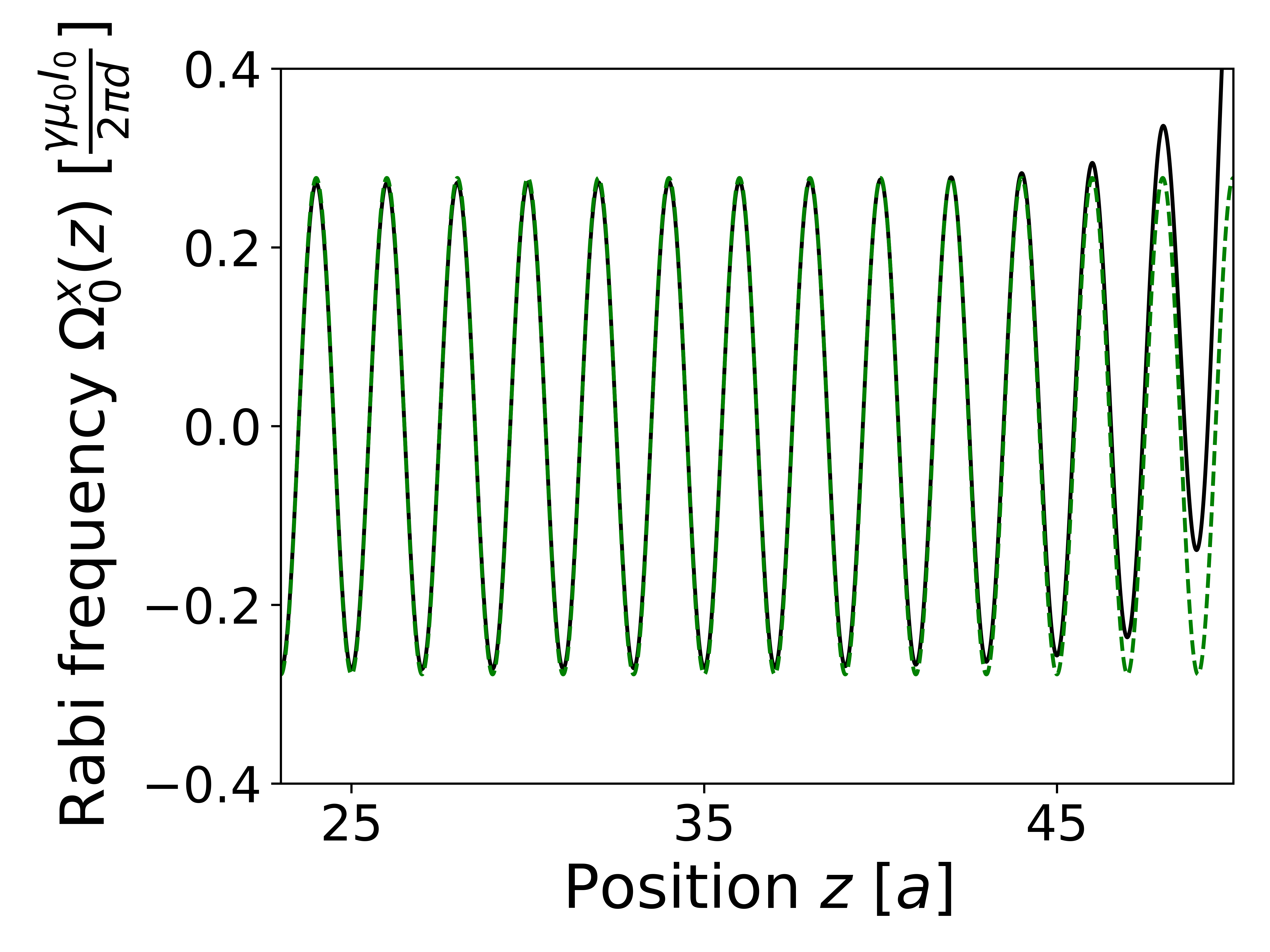
In the center region, where finite-size effects are negligible, the Rabi frequencies and are approximately given by
| (36) | |||||
| (37) |
The expressions (36) and (37) become exact in the limit of infinitely many wires, . For all practical purposes considered in this work, is very small such that and it may be safely neglected.
Appendix E Implementation II: Surface acoustic waves
E.1 Magnetization dynamics and effective magnetic field
Constitutive relations for magnetoelastic couplings.—The governing constitutive relations for magnetostriction [80] read
| (38) | |||||
| (39) |
where , , and denote the stress tensor, the magnetic induction, the magnetic field (intensity vector) generated by a magnetoelastic wave and the effective piezomagnetic tensor, respectively. is the magnetic permeability and the strain field is defined as .
Given Eq. (39), we provide an estimate for the effective driving field in the ferromagnet,
| (40) |
where denotes the magnetoelastic constant, is the wavevector and denotes the amplitude of the displacement field. For small strain-field amplitudes and a magnetoelastic constant T, this magnitude can be estimated as T [46].
At ferromagnetic resonance, the effective magnetic field can be significantly enhanced. The response of a ferromagnet to small time-varying magnetic fields can be described with the aid of Eq. (7). The resulting dynamical component of the magnetization is given by
| (41) |
where denotes the Polder susceptibility which describes the magnetic response of a ferromagnet to small time-varying magnetic fields perpendicular to the magnetization equilibrium direction [46]. In practical terms this means that the resulting effective magentic field can be enhanced by about two orders of magnitude.
In a next step, the field at the 2DEG is then calculated from the field distribution at the ferromagnetic thin film by discretizing the field distribution at the film and summing up the dipole fields of these volume elements. At high strain amplitudes and a magnetoelastic constant T, the relevant magnitude of the field at the 2DEG can be numerically estimated as mT. In our numerical calculations, the amplitude of the displacement field, the magnetoelastic coupling constant and the wavevector are input parameters which determine the microwave field strength at the ferromagnetic layer.
E.2 Strain-induced potentials
Starting from Eq. (8) and in a suitable rotating frame, we obtain
| (42) | |||||
with and . Following the procedure outlined in Refs. [49, 50] and using results from [17], we derive an effective time-independent Hamiltonian up to second order in which reads
| (43) |
with , , and . For typical parameter values , and , we obtain the simplified form
| (44) |
which coincides with the result given in Eq. (9). Writing Eq. (44) in the form , we find that the spin-dependent potential amplitudes read
| (45) |
The resulting trap depths are depicted in Fig. 5.
E.3 Stability analysis of hybrid magnetic and strain-induced traps
The discussion in this section completes the discussion of hybrid magnetic and strain-induced traps and is devoted to the stability analysis of such traps, meaning whether or not electrons can be trapped in time-dependent trapping potentials of the kind of those featured in Eq. (8).

Starting from Eq. (8), we would like to predict whether a given set of parameters gives rise to a stable (hybrid strain-induced and magnetic) trap or not. To this end, we first derive the coupled Heisenberg equations of motion for the set of observables within a RWA.
Equations of motion.—In order to determine the EOMs of interest, we consider the time evolution () of the operators which is given by the Heisenberg EOMs,
with and assuming that there exists no significant correlation between external and internal DOFs, i.e., decorrelated expressions such as, e.g., .
Two limiting cases.—We consider the two limiting cases (i) and (ii) : (i) At , we recover a Hamiltonian which is discussed in great detail in Ref. [17]; in the limit , the Heisenberg EOMs yield a Mathieu equation [81] whose stability diagram in terms of and is well-known, where denotes the speed of sound. (ii) For and in the large-detuning regime , an EOM can be derived which corresponds for a given spin state to a Hamiltonian of the form . Intuitively, these results agree very well with our expectation, since the case (i) coincides with a result known from the physics of trapped ions; this is not surprising since only the electric field contributes. On the other hand, case (ii) reproduces an effective Hamiltonian which is very familiar from optical lattices for cold (neutral) atoms [1]; this finding, in turn, underlines the close relation between the proposed magnetic traps and optical dipole traps which are both based on the AC Stark effect. In general, i.e., , the EOM leads to more involved dynamics. By adiabatic elimination of the internal DOFs, we obtain [corresponding to the constructive case in Eq. (45)] an EOM of the form
| (46) |
with stability parameters and and dimensionless quantities and . The ratio is typically small in the RWA regime. Based on Eq. (46), we extract stability diagrams (to predict the stability of solutions to Eq. (46)) in terms of and . These diagrams can have an intricate structure, see also Ref. [82, 83]. Here, we are mainly interested in the prediction of parameter constellations that give rise to stable solutions of Eq. (46). A prototypical stability diagram is shown in Fig. 8 for . It can be seen that a cut in Fig. 8 reproduces the well-known result that stable behaviour of solutions to the Mathieu equation occurs at for . At , the stability properties can be rather sensitive to slight changes in . An operation in the stable regime therefore requires a balanced choice of these parameters. However, Fig. 8 shows that several values support a range of stable values which indicates that operation in a stable regime is possible for a significant range of parameters. Moreover, the numerical parameters used in Fig. 4 give rise to which allows for stable trajectories for many different . We conclude that, even in the presence of induced electric fields, stable magnetic traps can be operated.