跳到论文正文
W Papers独立论文阅读器 arXiv:1804.07416 论文正文 计算阅读时间 · 0%
引用这篇论文根据当前论文元数据生成,正式投稿前建议核对。


License: CC BY-NC-SA 4.0
arXiv:1804.07416v2 [math.ST] 22 Nov 2019

Variable Selection via Adaptive False Negative Control in Linear Regression

X. Jessie Jeng??    Xiongzhi Chen
Abstract

Variable selection methods have been developed in linear regression to provide sparse solutions. Recent studies have focused on further interpretations on the sparse solutions in terms of false positive control. In this paper, we consider false negative control for variable selection with the goal to efficiently select a high proportion of relevant predictors. Different from existing studies in power analysis and sure screening, we propose to directly estimate the false negative proportion (FNP) of a decision rule and select the smallest subset of predictors that has the estimated FNP less than a user-specified control level. The proposed method is adaptive to the user-specified control level on FNP by selecting less candidates if a higher level is implemented. On the other hand, when data has stronger effect size or larger sample size, the proposed method controls FNP more efficiently with less false positives. New analytic techniques are developed to cope with the major challenge of FNP control when relevant predictors cannot be consistently separated from irrelevant ones. Our numerical results are in line with the theoretical findings.

keywords
[class=MSC] Primary 62J07 ; secondary 62F03
keywords
Debiased Lasso , FNC-Reg , Post-Selection Inference , Variable Screening

and

Department of Statistics, North Carolina State University, Raleigh, NC 27695
??

Department of Mathematics and Statistics
Washington State University, Pullman, WA 99164
??

Contents

1 Introduction

We consider a sparse linear model

𝐲=𝐗​𝜷+𝜺,\mathbf{y}=\mathbf{X}\boldsymbol{\beta}+\boldsymbol{\varepsilon}, (1.1)

where 𝐲=(y1,…,yn)T\mathbf{y}=(y_{1},\ldots,y_{n})^{T} is the vector of nn observations of response, 𝐗=[𝐱1,…,𝐱p]∈ℝn×p\mathbf{X}=[\mathbf{x}_{1},\ldots,\mathbf{x}_{p}]\in\mathbb{R}^{n\times p} is the design matrix, 𝜷=(β1,…,βp)T\boldsymbol{\beta}=(\beta_{1},\ldots,\beta_{p})^{T} is the vector of unknown coefficients, and 𝜺∼𝒩n​(0,σ2​𝐈)\boldsymbol{\varepsilon}\sim\mathcal{N}_{n}\left(0,\sigma^{2}\mathbf{I}\right) is the vector of random errors. We assume σ2=O⁡(1)\sigma^{2}=O\left(1\right). Let I1={1≤j≤p:βj≠0}I_{1}=\left\{1\leq j\leq p:\beta_{j}\neq 0\right\} be the set of indices for non-zero coefficients with cardinality s=|I1|s=|I_{1}| and I0={1≤j≤p:βj=0}I_{0}=\left\{1\leq j\leq p:\beta_{j}=0\right\} with cardinality p0=|I0|p_{0}=\left|I_{0}\right|.

Variable selection methods often provide sparse solutions for the estimation of 𝜷\boldsymbol{\beta}. The non-zero elements of an estimate correspond to variables selected as candidates for relevant predictors. A great amount of literature with many fruitful ideas has contributed to the development of sparse solutions to accommodate the underlying features of the data. We refer to [5] and the references therein for a nice introduction.

Given a selection result, a false positive (FP) occurs when an irrelevant predictor is selected, and a false negative (FN) occurs when a relevant predictor is not selected. It is natural to interpret a selection result in terms of false positive or false negative control, and exciting progress has emerged for false positive control, e.g. [3], [4], [9], [17], [24], [32], [38]. However, the study for efficient false negative control remains relatively underdeveloped.

False negative control is important in many real applications and sometimes a more serious concern than false positive control. For example, in pre-surgical brain mapping with functional MRI, the primary goal is to reduce false negatives where genuine functional areas are not identified. This is because neurosurgical patients are more likely to experience significant harm from mistakenly deeming a region to be functionally uninvolved and subsequently resecting critical tissue than from incorrectly assigning function to an uninvolved region [25, 26, 31]. Another example where false negative control is of main concern is in the exploratory stage of high-dimensional data analysis, where pre-screening is often conducted to reduce data dimension while keeping a high proportion of true signal variables for follow-up studies.

The problem of false negative control is conceptually related but methodologically very different from Sure Screening in, e.g., [14, 15]. Sure Screening aims to reduce the data dimension by removing only irrelevant predictors. For instance, the Sure Independence Screening procedure in [14] ranks variables by estimated marginal regression coefficients and selects the top dd variables where dd is fixed at n−1n-1 or n/log⁡nn/\log n. It has been proved that under certain conditions, the screening procedure has eliminated only irrelevant predictors with high probability. The false negative control problem considered here focuses on selecting a high proportion of relevant predictors without including many unnecessary irrelevant predictors. It may be regarded as a more refined screening procedure with a data-adaptive selection rule instead of a fixed dd.

We use false negative proportion (FNP) as a measure for false negative control. For a given selection rule, FNP is defined as the ratio of the number of false negatives to the total number of relevant predictors. FNP takes values in [0,1][0,1] and is equivalent to 1−𝖲𝖾𝗇𝗌𝗂𝗍𝗂𝗏𝗂𝗍𝗒1-\mathsf{Sensitivity} in binary classification framework. Our work starts with consistently estimating FNP for a given selection rule. To achieve this, we develop novel analyses on the tail behavior of the empirical processes associated with FNP. Based on the estimation of FNP, we develop a new variable selection procedure to control FNP at a user-specified level. If users can tolerate more false negatives, they may implement lower control levels on FNP in the procedure and select less candidates for relevant predictors. On the other hand, if the effect of relevant predictors gets stronger or sample size increases, the procedure controls FNP more efficiently with less false positives.

An important component of the proposed FNP control method is an estimator for the number of relevant predictors. We provide a consistent estimator for dependent test statistics, for which we adopt the recently developed debiased Lasso estimates [20, 34, 37].

Although FNP, by definition, is equivalent to the power in (single) hypothesis testing, our proposed study on FNP control is very different from the existing power analysis in hypothesis testing. In the latter, a decision rule is built upon Type I error control and followed by power calculation with assumptions on the effect size. For such methods to control FNP in addition to controlling family-wise Type I error when multiple hypotheses are considered, the effect sizes of relevant variables need to be larger enough to ensure essentially perfect separation of relevant and irrelevant variables. The proposed method, on the other hand, directly bound the estimated FNP at a user-specified level, which allows a more effective control on FNP. Our condition on effect size for FNP control is shown to be weaker than the existing beta-min conditions that are required for perfect separation of relevant and irrelevant variables.

The rest of the paper is organized as follows. Section 2 presents FNP estimation in two steps: (1) constructing test statistics for regression coefficients and (2) approximating FNP based on the test statistics. Section 3 develops a variable selection method to control FNP at a user-specified level and a computational algorithm to implement the method. Section 4 presents the finite-sample performance of the proposed method in simulation. Conclusion and further discussion are provided in Section 5. Proofs for the main theoretical results are presented in Section 6. Extra technical details are provided in Appendix.

2 False Negative Proportion Estimation

Recall that for a selection rule, FNP is the ratio of the number of false negatives to the total number of relevant predictors. In this section, we rank the predictors based on the debiased Lasso estimates and approximate FNP at a given cut-off point on the list of ranked predictors.

2.1 Test Statistics Based on Debiased Lasso Estimates

Recall model (1.1). The well-known Lasso estimator is

𝜷^=𝜷^​(λ)=arg⁡min𝜷∈ℝp⁡(‖𝐲−𝐗​𝜷‖22/n+2​λ​‖𝜷‖1),\hat{\boldsymbol{\beta}}=\hat{\boldsymbol{\beta}}(\lambda)=\arg\min_{\boldsymbol{\beta}\in\mathbb{R}^{p}}(\|\mathbf{y}-\mathbf{X}\boldsymbol{\beta}\|_{2}^{2}/n+2\lambda\|\boldsymbol{\beta}\|_{1}), (2.1)

where λ\lambda is a tuning parameter [33]. Recently, the debiased Lasso estimator has been developed to mitigate the bias of Lasso estimator [34, 37]. The debiased Lasso estimator is defined as

𝐛^=(b^1,…,b^p)T=𝜷^+n−1​𝚯^​𝐗T​(𝐲−𝐗​𝜷^),\hat{\mathbf{b}}=\left(\hat{b}_{1},\ldots,\hat{b}_{p}\right)^{T}=\hat{\boldsymbol{\beta}}+n^{-1}\hat{\boldsymbol{\Theta}}\mathbf{X}^{T}(\mathbf{y}-\mathbf{X}\hat{\boldsymbol{\beta}}), (2.2)

where 𝚯^∈ℝp×p\hat{\boldsymbol{\Theta}}\in\mathbb{R}^{p\times p} is an estimate for the precision matrix of the predictors and can be obtained via nodewise regression on 𝐗\mathbf{X} as in [28]. Let 𝚺^=n−1​𝐗T​𝐗\hat{\boldsymbol{\Sigma}}=n^{-1}\mathbf{X}^{T}\mathbf{X}. It has been shown that

n(𝐛^−𝜷)=n−1/2𝚯^𝐗T𝜺−𝜹=𝐰−𝜹,\sqrt{n}(\hat{\mathbf{b}}-\boldsymbol{\beta})=n^{-1/2}\hat{\boldsymbol{\Theta}}\mathbf{X}^{T}\boldsymbol{\varepsilon}-\boldsymbol{\delta}=\mathbf{w}-\boldsymbol{\delta}, (2.3)

where

𝐰|𝐗∼𝒩p(0,σ2𝛀^),𝛀^=𝚯^𝚺^𝚯^T,\mathbf{w}|\mathbf{X}\sim\mathcal{N}_{p}(0,\sigma^{2}\hat{\boldsymbol{\Omega}}),\qquad\hat{\boldsymbol{\Omega}}=\hat{\boldsymbol{\Theta}}\hat{\boldsymbol{\Sigma}}\hat{\boldsymbol{\Theta}}^{T},

and

𝜹=(δ1,…,δp)T=n​(𝚯^​𝚺^−𝐈)​(𝜷^−𝜷).\boldsymbol{\delta}=\left(\delta_{1},\ldots,\delta_{p}\right)^{T}=\sqrt{n}(\hat{\boldsymbol{\Theta}}\hat{\boldsymbol{\Sigma}}-\mathbf{I})(\hat{\boldsymbol{\beta}}-\boldsymbol{\beta}). (2.4)

Under certain conditions, ‖𝜹‖∞=op​(1)\|\boldsymbol{\delta}\|_{\infty}=o_{p}(1), which implies the asymptotic normality of 𝐛^\hat{\mathbf{b}} [6, 20, 21, 34, 37]. We present the set of conditions from [21] as A1) - A3) in Appendix A.1.

In this paper, we obtain test statistics for 𝜷\boldsymbol{\beta} using the standardized debiased Lasso estimator as

zj=nb^jσ−1𝛀^j​j−1/2 for1≤j≤pz_{j}=\sqrt{n}\hat{b}_{j}\sigma^{-1}\hat{\boldsymbol{\Omega}}_{jj}^{-1/2}\text{ \ for}\qquad 1\leq j\leq p (2.5)

where 𝛀^j​j\hat{\boldsymbol{\Omega}}_{jj} denotes the (j,j)\left(j,j\right) entry of 𝛀^\hat{\boldsymbol{\Omega}}. Therefore, for each 1≤j≤p1\leq j\leq p,

zj=μj+wj′−δj′,z_{j}=\mu_{j}+w_{j}^{\prime}-\delta_{j}^{\prime},

where, given 𝐗\mathbf{X},

wj′=wjσ​𝛀^j​j∼𝒩(0,1), δj′=δjσ​𝛀^j​j and μj=n​βjσ​𝛀^j​j.w_{j}^{\prime}=\frac{w_{j}}{\sigma\sqrt{\boldsymbol{\hat{\Omega}}_{jj}}}\sim\mathcal{N}(0,1),\text{ \ }\delta_{j}^{\prime}=\frac{\delta_{j}}{\sigma\sqrt{\boldsymbol{\hat{\Omega}}_{jj}}}\text{ \ and\ \ \ }\mu_{j}=\frac{\sqrt{n}\beta_{j}}{\sigma\sqrt{\boldsymbol{\hat{\Omega}}_{jj}}}. (2.6)

2.2 Approximating False Negative Proportion

We aim to determine a cut-off value for the realized test statistics to control false negative proportion (FNP) at an user-specified level. For this purpose, we first study the consistent estimation of 𝖥𝖭𝖯\mathsf{FNP}. For any t>0t>0, define

R(t)=∑j=1p1{|zj|>t},𝖳𝖯(t)=∑j∈I11{|zj|>t},𝖥𝖭(t)=∑j∈I11{|zj|≤t},𝖥𝖯(t)=∑j∈I01{|zj|>t}.R\left(t\right)=\sum_{j=1}^{p}1_{\left\{\left|z_{j}\right|>t\right\}},\quad\mathsf{TP}\left(t\right)=\sum_{j\in I_{1}}1_{\left\{\left|z_{j}\right|>t\right\}},\quad\mathsf{FN}\left(t\right)=\sum_{j\in I_{1}}1_{\left\{\left|z_{j}\right|\leq t\right\}},\quad\mathsf{FP}\left(t\right)=\sum_{j\in I_{0}}1_{\left\{\left|z_{j}\right|>t\right\}}.

Note that 𝖥𝖭⁡(t)\mathsf{FN}\left(t\right) is unobservable as I1I_{1} is unknown, and that the dependence among zjz_{j}’s also affect 𝖥𝖭⁡(t)\mathsf{FN}\left(t\right). It is easy to see that

𝖥𝖭⁡(t)=s−𝖳𝖯⁡(t)=s−[R⁡(t)−𝖥𝖯⁡(t)]\mathsf{FN}\left(t\right)=s-\mathsf{TP}\left(t\right)=s-\left[R\left(t\right)-\mathsf{FP}\left(t\right)\right] (2.7)

and

𝖥𝖭𝖯⁡(t)=𝖥𝖭⁡(t)s=1−R⁡(t)−𝖥𝖯⁡(t)s.\mathsf{FNP}\left(t\right)=\frac{\mathsf{FN}\left(t\right)}{s}=1-\frac{R\left(t\right)-\mathsf{FP}\left(t\right)}{s}. (2.8)

Since R⁡(t)R\left(t\right) is directly observable from the data, the unknown quantities in (2.8) are 𝖥𝖯⁡(t)\mathsf{FP}\left(t\right) and ss. We propose to substitute 𝖥𝖯⁡(t)\mathsf{FP}\left(t\right) in (2.7) by 2​(p−s)​Φ​(−t)2(p-s)\Phi\left(-t\right), where Φ⁡(⋅)\Phi(\cdot) is the cumulative distribution function (CDF) of a standard Normal random variable, because zjz_{j} is asymptotically standard Normal for j∈I0j\in I_{0}. Further, we can plug in an estimator s^\hat{s} for ss, which results in the estimator

𝖥𝖭𝖯^​(t)=1−R⁡(t)−2​(p−s^)​Φ​(−t)s^.\widehat{\mathsf{FNP}}\left(t\right)=1-\frac{R\left(t\right)-2(p-\hat{s})\Phi\left(-t\right)}{\hat{s}}. (2.9)

From the definitions of 𝖥𝖭𝖯⁡(t)\mathsf{FNP}\left(t\right) and 𝖥𝖭𝖯^​(t)\widehat{\mathsf{FNP}}\left(t\right), it can be shown that
|𝖥𝖭𝖯^​(t)−𝖥𝖭𝖯⁡(t)|=oP​(1)\left|\widehat{\mathsf{FNP}}\left(t\right)-\mathsf{FNP}\left(t\right)\right|=o_{P}(1) is implied by

s−1​|𝖥𝖯⁡(t)−2​p0​Φ​(−t)|=oP​(1)and|s^/s−1|=oP​(1).s^{-1}\left|\mathsf{FP}(t)-2p_{0}\Phi(-t)\right|=o_{P}\left(1\right)\qquad\text{and}\qquad|\hat{s}/s-1|=o_{P}(1). (2.10)

Because 𝖥𝖯⁡(t)\mathsf{FP}(t) is the summation of p0p_{0} terms and ss can be much smaller than p0p_{0}, approximating 𝖥𝖯⁡(t)/s\mathsf{FP}(t)/s requires more delicate analysis than approximating 𝖥𝖯⁡(t)/p0\mathsf{FP}(t)/p_{0}, which has been studied in the literature for False Discovery Proportion (FDP) control (e.g. [13]). Also, the dependence among test statistics {zj}j=1p\{z_{j}\}_{j=1}^{p} adds another layer of difficulty.

In this paper, we consider s=p1−ηs=p^{1-\eta} for some η∈(0,1)\eta\in(0,1), so that the number of relevant predictors is of a smaller order than the total number of variables. On the other hand, we consider tt values calibrated as t=tξ=2​ξ​log⁡pt=t_{\xi}=\sqrt{2\xi\log p} for some ξ>0\xi>0, so that the scale of tt is comparable to that of the extreme value of pp independent standard Gaussian variables. Such calibration has been utilized to study the detection of Gaussian mixtures [2, 7, 12], and to analyze variable selection consistency in linear regression [23]. In this paper, we adopt the calibration to study the estimation of FNP in linear regression.

Further, define the precision matrix of the predictors as 𝚯\boldsymbol{\Theta} and let

sj=|{k≠j:𝚯j​k≠0}|andsm​a​x=max1≤j≤p⁡sj.s_{j}=\left|\left\{k\neq j:\boldsymbol{\Theta}_{jk}\neq 0\right\}\right|\qquad\text{and}\qquad s_{max}=\max_{1\leq j\leq p}s_{j}.

Namely, the parameter sm​a​xs_{max} represents the row-sparsity of the precision matrix, which contributes to the strength of the dependence among the test statistics. Define

γ1∗=2​η−min⁡{1,log⁡(n/sm​a​x)2​log⁡p},γ2∗=2−2​η−log⁡n2​log⁡p,\gamma^{*}_{1}=2\eta-\min\{1,{\log(n/s_{max})\over 2\log p}\},\qquad\gamma^{*}_{2}=2-2\eta-{\log n\over 2\log p},

and

γ∗=max⁡{γ1∗,γ2∗}.\gamma^{*}=\max\{\gamma^{*}_{1},\gamma^{*}_{2}\}. (2.11)

The next theoretical result demonstrates the range of tt values in which the first equation s−1​|𝖥𝖯⁡(t)−2​p​Φ​(−t)|=oP​(1)s^{-1}\left|\mathsf{FP}(t)-2p\Phi(-t)\right|=o_{P}\left(1\right) in (2.10) is achievable.

Theorem 2.1.

Consider model (1.1) and the test statistics {zj}j=1p\{z_{j}\}_{j=1}^{p} in (2.5). Assume conditions A1) through A3) in Appendix A.1 for the asymptotic normality of {zj}j=1p\{z_{j}\}_{j=1}^{p}. Let s=p1−ηs=p^{1-\eta} for some η∈(0,1)\eta\in(0,1) and t=tξ=2​ξ​log⁡pt=t_{\xi}=\sqrt{2\xi\log p} for ξ>0\xi>0. Assume ξ>min⁡{η,γ∗}\xi>\min\{\eta,\gamma^{*}\} for γ∗\gamma^{*} in (2.11), then

s−1​|𝖥𝖯⁡(tξ)−2​p0​Φ​(−tξ)|=oP​(1).s^{-1}\left|\mathsf{FP}(t_{\xi})-2p_{0}\Phi(-t_{\xi})\right|=o_{P}\left(1\right). (2.12)

Because 𝖥𝖯⁡(t)\mathsf{FP}(t) is the summation of p0p_{0} indicator functions and p0≫s(=p1−η)p_{0}\gg s(=p^{1-\eta}), 𝖥𝖯⁡(t)/s\mathsf{FP}(t)/s blows up at constant tt. Theorem 2.1 says that the approximation of 𝖥𝖯⁡(t)/s\mathsf{FP}(t)/s is achievable for tt at the scale of tξt_{\xi}. This is substantially different from the existing study of FDP control, where the approximation of 𝖥𝖯⁡(t)/p0\mathsf{FP}(t)/p_{0} and R⁡(t)/p0R(t)/p_{0} are studied at constant tt.

The condition ξ>min⁡{η,γ∗}\xi>\min\{\eta,\gamma^{*}\} can be decomposed as follows. When η≤γ∗\eta\leq\gamma^{*}, we have ξ>η\xi>\eta, and the claim in (2.12) follows by showing that s−1​𝖥𝖯​(tξ)=op​(1)=s−1​p0​Φ​(−tξ)s^{-1}\mathsf{FP}(t_{\xi})=o_{p}(1)=s^{-1}p_{0}\Phi(-t_{\xi}). On the other hand, when η>γ∗\eta>\gamma^{*} and γ∗<ξ≤η\gamma^{*}<\xi\leq\eta, more delicate analysis is needed to study the variability of 𝖥𝖯⁡(tξ)\mathsf{FP}(t_{\xi}). The condition ξ>γ1∗\xi>\gamma^{*}_{1} essentially controls the variability of s−1​𝖥𝖯𝗐′​(tξ)s^{-1}\mathsf{FP_{w^{\prime}}}(t_{\xi}), where 𝐰′\bf{w}^{\prime} is the Gaussian component of 𝐳\mathbf{z} as in (2.6) and 𝖥𝖯𝗐′(tξ)=∑j∈I01{|w′j|>tξ}\mathsf{FP_{w^{\prime}}}(t_{\xi})=\sum_{j\in I_{0}}1_{\left\{\left|w^{\prime}_{j}\right|>t_{\xi}\right\}}. The condition ξ>γ2∗\xi>\gamma^{*}_{2} controls the cumulative errors caused by the component 𝜹′\boldsymbol{\delta}^{\prime} of 𝐳\mathbf{z}.

Existing study in [23] has shown optimal phase diagram in (ξ,η)(\xi,\eta) for high-dimensional variable selection. Their work, however, focuses on scenarios with ξ>η\xi>\eta. We extend the analysis to the more challenging case with γ∗<ξ≤η\gamma^{*}<\xi\leq\eta, for which we study the variability of s−1​𝖥𝖯𝗐′​(tξ)s^{-1}\mathsf{FP_{w^{\prime}}}(t_{\xi}) under the dependence of test statistics. Recall the covariance matrix σ2​𝛀^\sigma^{2}\hat{\boldsymbol{\Omega}} in (2.3). Since 𝛀^=𝚯^​𝚺^​𝚯^T\hat{\boldsymbol{\Omega}}=\hat{\boldsymbol{\Theta}}\hat{\boldsymbol{\Sigma}}\hat{\boldsymbol{\Theta}}^{T} and that 𝚺^\hat{\boldsymbol{\Sigma}} is not a sparse matrix, σ2​𝛀^\sigma^{2}\hat{\boldsymbol{\Omega}} is not sparse or possessing any well-known structures. The study in [23] imposes conditions on the covariance matrix of predictors that essentially prohibit excessive signal cancellations when performing marginal regression. Our condition of dependence, on the other hand, demonstrate the effect of the sparsity of precision matrix (sm​a​xs_{max}) through γ∗\gamma^{*}. Overall, ξ>min⁡{η,γ∗}\xi>\min\{\eta,\gamma^{*}\} is easier to be satisfied with larger nn, smaller pp, or smaller sm​a​xs_{max}.

To achieve the second equation in (2.10), we modify the estimator introduced in [29] and study its consistency for estimating ss in our setting. We refer to the modified estimator as the MR estimator. Recall the standardized debiased Lasso estimator zj=nb^jσ−1𝛀^j​j−1/2,1≤j≤pz_{j}=\sqrt{n}\hat{b}_{j}\sigma^{-1}\hat{\boldsymbol{\Omega}}_{jj}^{-1/2},1\leq j\leq p. Let Fp(t)=p−1∑j=1p1{|zj|>t}F_{p}(t)=p^{-1}\sum_{j=1}^{p}1_{\{|z_{j}|>t\}} and σ¯​(t)=2​Φ¯​(t)​(1−2​Φ¯​(t))\bar{\sigma}\left(t\right)=\sqrt{2\bar{\Phi}(t)\left(1-2\bar{\Phi}(t)\right)}, where Φ¯​(t)=1−Φ​(t)\bar{\Phi}(t)=1-\Phi(t). The MR estimator for the portion of relevant predictors (π=s/p\pi=s/p) is constructed as

π^=supt>0Fp​(t)−2​Φ¯​(t)−cp​σ¯​(t)1−2​Φ¯​(t),\hat{\pi}=\sup_{t>0}{\frac{F_{p}(t)-2\bar{\Phi}(t)-c_{p}\bar{\sigma}\left(t\right)}{1-2\bar{\Phi}(t)}}, (2.13)

where cpc_{p} is a bounding sequence pre-specified as follows. Define Gp(t)=p−1∑j=1p1{|wj′|>t}G_{p}\left(t\right)=p^{-1}\sum_{j=1}^{p}1_{\{|w_{j}^{\prime}|>t\}},

𝖧⁡(t)=Gp​(t)−2​Φ¯​(t)σ¯​(t),andVp=supt>0𝖧⁡(t).\mathsf{H}(t)={\frac{G_{p}(t)-2\bar{\Phi}(t)}{\bar{\sigma}\left(t\right)}},\qquad\text{and}\qquad V_{p}=\sup_{t>0}\mathsf{H}(t). (2.14)

Set cpc_{p} as the (1−αp)(1-\alpha_{p})-th quantile of VpV_{p} for αp=o⁡(1)\alpha_{p}=o(1), so that P⁡(Vp>cp)=αp→0P(V_{p}>c_{p})=\alpha_{p}\rightarrow 0 as p→∞p\rightarrow\infty. In other words, cpc_{p} can be looked upon as an upper bound for VpV_{p} probabilistically, and the implement of cpc_{p} in (2.13) eventually controls over-estimation on π\pi.

Compared to the original MR estimator in [29], the key modification in (2.13) and (2.14) is the use of Fp​(t)F_{p}(t) and Gp​(t)G_{p}\left(t\right), two empirical processes each with dependent random summands. Naturally, this requires different techniques to find {cp}p≥1\left\{c_{p}\right\}_{p\geq 1}. The setting in [29] considers independent pp-values that are uniformly distributed under the null hypothesis. Since the limiting distribution of the uniform empirical process with independent summands is known and has an analytic expression, a bounding sequence can be directly found from the distribution in the construction of the original MR estimator. However, in our settings {zj}j=1p\left\{z_{j}\right\}_{j=1}^{p} are dependent, and the exact distributions of {b^j}j=1p\{\hat{b}_{j}\}_{j=1}^{p} are unspecified.

In fact, {b^j}j=1p\{\hat{b}_{j}\}_{j=1}^{p} asymptotically has covariance matrix σ2​𝛀^=σ2​𝚯^​𝚺^​𝚯^T\sigma^{2}\hat{\boldsymbol{\Omega}}=\sigma^{2}\hat{\boldsymbol{\Theta}}\hat{\boldsymbol{\Sigma}}\hat{\boldsymbol{\Theta}}^{T}. In theory, |𝛀^i​j−𝚯i​j|=op​(1)|\hat{\boldsymbol{\Omega}}_{ij}-\boldsymbol{\Theta}_{ij}|=o_{p}(1) for any (i,j)(i,j) under conditions A1) through A3) in Appendix A.1. However, 𝛀^\hat{\boldsymbol{\Omega}} itself is neither diagonal nor sparse, and the approximation errors of all the elements in 𝛀^\hat{\boldsymbol{\Omega}} add up to influence VpV_{p} . Note that VpV_{p} is the higher criticism statistic of [12] based on the Gaussian component 𝐰′\mathbf{w}^{\prime} of 𝐳\mathbf{z}. Unfortunately, existing techniques for higher criticism statistic under short-range and long-range dependence [18] cannot be applied here because our test statistics with covariance matrix σ2​𝛀^\sigma^{2}\hat{\boldsymbol{\Omega}} cannot be partitioned as in [18].

In this paper, we employ a discretization technique adopted from [1] to derive bounds on the variance of a discretized {𝖧⁡(t):t>0}\left\{\mathsf{H}(t):t>0\right\} and define a discretized version of VpV_{p} as

Vp∗=max⁡{𝖧⁡(t):t∈[τ0​log⁡p,τ1​log⁡p]∩ℕ}V_{p}^{\ast}=\max\left\{\mathsf{H}(t):t\in\left[\sqrt{\tau_{0}\log p},\sqrt{\tau_{1}\log p}\right]\cap\mathbb{N}\right\} (2.15)

for two positive constants τ0\tau_{0} and τ1\tau_{1} such that 0<τ0<τ10<\tau_{0}<\tau_{1}. Then, a discretized version of the MR estimator is defined as

π^∗=max⁡{Fp​(t)−2​Φ¯​(t)−cp∗​σ¯​(t)1−2​Φ¯​(t):t∈[τ0​log⁡p,τ1​log⁡p]∩ℕ},\hat{\pi}^{\ast}=\max\left\{\frac{F_{p}(t)-2\bar{\Phi}(t)-c_{p}^{\ast}\bar{\sigma}\left(t\right)}{1-2\bar{\Phi}(t)}:t\in\left[\sqrt{\tau_{0}\log p},\sqrt{\tau_{1}\log p}\right]\cap\mathbb{N}\right\}, (2.16)

where cp∗c_{p}^{\ast} is the (1−αp)(1-\alpha_{p})-th quantile of Vp∗V_{p}^{\ast} for αp=o⁡(1)\alpha_{p}=o(1). Let

μm​i​n=minj∈I1n|βj|σ−1𝚯j​j−1/2\mu_{min}=\min_{j\in I_{1}}\sqrt{n}\left|\beta_{j}\right|\sigma^{-1}\boldsymbol{\Theta}_{jj}^{-1/2} (2.17)

as a measure on the minimal effect size of relevant variables. The following theorem demonstrates the consistency of π^∗\hat{\pi}^{\ast}. Its proof is presented in Section 6.2.

Theorem 2.2.

Assume conditions A1) through A3) in Appendix A.1 for the asymptotic normality of {zj}j=1p\{z_{j}\}_{j=1}^{p}. Let s=p1−ηs=p^{1-\eta} for some η∈(0,1)\eta\in(0,1) and μm​i​n≥2​(γ∗+c)​log⁡p\mu_{min}\geq\sqrt{2(\gamma^{*}+c)\log p} for μm​i​n\mu_{min} and γ∗\gamma^{*} in (2.17) and (2.11) and some constant c>0c>0. Then π^∗\hat{\pi}^{\ast} with bounding sequence cp∗c_{p}^{\ast} at the order of (smax/n)1/4​log⁡p(s_{\max}/n)^{1/4}\log p, τ0∈(2​γ∗,2​γ∗+c)\tau_{0}\in(2\gamma^{*},2\gamma^{*}+c), and τ1>2​(γ∗+c)\tau_{1}>2(\gamma^{*}+c) consistently estimates the proportion π\pi of relevant predictors, i.e., for any δ>0\delta>0,

P⁡(|π^∗/π−1|<δ)→1P(|\hat{\pi}^{\ast}/\pi-1|<\delta)\rightarrow 1

and, consequently, s^=π^∗​p\hat{s}=\hat{\pi}^{*}p satisfies

P⁡(|s^/s−1|<δ)→1.P(|\hat{s}/s-1|<\delta)\rightarrow 1.

Note that the order of cp∗c^{*}_{p} shows the effects of sparsity of the precision matrix (sm​a​xs_{max}), sample size (nn), and dimensionality (pp) on Vp∗V_{p}^{*}. The condition μm​i​n≥2​(γ∗+c)​log⁡p\mu_{min}\geq\sqrt{2(\gamma^{*}+c)\log p} shows that consistent estimation of ss gets easier with smaller sm​a​xs_{max}, larger nn, and smaller pp.

In summary, Theorem 2.1 and Theorem 2.2 facilitate the two equations in (2.10) for FNP(t)(t) estimation by 𝖥𝖭𝖯^​(t)\widehat{\mathsf{FNP}}(t). Note that in practice we will need to simulate VpV_{p} and cpc_{p} to derive the estimated ss and 𝖥𝖭𝖯⁡(t)\mathsf{FNP}(t). Please refer to Section 3.2 for details of the numerical implementation.

3 FNP Control at a User-Specified Level

In this section, we introduce a new method for FNP control at a user-specified level in high-dimensional regression. We say that a variable selection method asymptotically controls FNP at a pre-specified level ϵ∈(0,1)\epsilon\in(0,1) if the FNP of its selection outcome satisfies

P⁡(𝖥𝖭𝖯<ϵ)→1.P\left(\mathsf{FNP}<\epsilon\right)\rightarrow 1.

Such methods are useful in applications where data dimensions need to be largely reduced for subsequent analyses while controlling false negatives at a tolerable level.

3.1 The FNC-Reg Procedure

Based on the approximation results of FNP, we propose the False Negative Control for Regression (FNC-Reg) procedure, which determines the cut-off threshold on the list of ranked {|zj|}j=1p\{|z_{j}|\}_{j=1}^{p} as

t∗​(ϵ)=sup{t:𝖥𝖭𝖯^​(t)≤ϵ}t^{\ast}(\epsilon)=\sup\left\{t:\widehat{\mathsf{FNP}}(t)\leq\epsilon\right\} (3.1)

for an user-specified ϵ∈(0,1)\epsilon\in(0,1). FNC-Reg selects predictors with |zj|>t∗​(ϵ)|z_{j}|>t^{\ast}(\epsilon).

It can be seen that FNC-Reg is a procedure built upon direct estimation of FNP and a user-specified control level of FNP. Given that 𝖥𝖭𝖯^​(t)\widehat{\mathsf{FNP}}(t) is non-increasing with tt, FNC-Reg selects the smallest subset of {zj}j=1p\{z_{j}\}_{j=1}^{p} such that the estimated FNP is less than ϵ\epsilon. Moreover, this procedure depends on user’s preference for the control level of FNP. Since t∗​(ϵ)t^{\ast}(\epsilon) is non-decreasing with ϵ\epsilon, if users can tolerate missing a higher proportion (larger ϵ\epsilon) of relevant variables, they may select less variables using the procedure. The selected subset of variables can be much smaller than the full set of variables, which corresponds to no false negatives. The next theorem shows that under certain conditions, the FNC-Reg procedure asymptotically controls the true FNP at the level of ϵ\epsilon.

Theorem 3.1.

Assume conditions A1) through A3) in Appendix A.1. Assume μm​i​n≥2​(γ∗+c)​log⁡p\mu_{min}\geq\sqrt{2(\gamma^{*}+c)\log p} for μm​i​n\mu_{min} and γ∗\gamma^{*} in (2.17) and (2.11) and some constant c>0c>0. Then t∗​(ϵ)t^{*}(\epsilon) determined by (3.1) with s^=π^∗​p\hat{s}=\hat{\pi}^{*}p satisfies

P⁡(𝖥𝖭𝖯⁡(t∗​(ϵ))≤ϵ)→1.P\left(\mathsf{FNP}(t^{\ast}(\epsilon))\leq\epsilon\right)\rightarrow 1. (3.2)

Consequently, t∗​(ϵ)t^{*}(\epsilon) determined by (3.1) with s^=π^​p\hat{s}=\hat{\pi}p and cp=cp∗c_{p}=c_{p}^{*} also satisfies

P⁡(𝖥𝖭𝖯⁡(t∗​(ϵ))≤ϵ)→1.P\left(\mathsf{FNP}(t^{\ast}(\epsilon))\leq\epsilon\right)\rightarrow 1. (3.3)

Result in (3.2) shows the FNP control by FNC-Reg when the discretized MR estimator is implemented in (2.9). (3.3) extends the result to FNC-Reg with the MR estimator.

We compare the condition on μmin\mu_{\min} in Theorem 3.1 with the beta-min condition of variable selection consistency. Our condition on μmin\mu_{\min} achieves the order O⁡((log⁡p)/n)O(\sqrt{(\log p)/n}) for βm​i​n\beta_{min}, which is the optimal oder for variable selection consistency [19, 35]. On the other hand, Our condition on μmin\mu_{\min} specifies the constant term 2​γ∗\sqrt{2\gamma^{*}} with γ∗\gamma^{*} in (2.11), while existing beta-min conditions for different methods have various constant terms that are often not fully specified. Therefore, we attempt to compare with the optimal constant term for variable selection consistency in the ideal setting, where the predictors (Xi​1,…,Xi​p)(X_{i1},\ldots,X_{ip}) are generated as i.i.d. samples from N⁡(0,Ip×p)N(0,I_{p\times p}). Existing study in, for example, [23] has shown that the optimal constant is 2+2​(1−η)\sqrt{2}+\sqrt{2(1-\eta)}, i.e. smaller η\eta (larger ss) makes it harder to perfectly separate all the signals from noise. Then, it follows that 2​γ∗<2+2​(1−η)\sqrt{2\gamma^{*}}<\sqrt{2}+\sqrt{2(1-\eta)} for any η∈(0,1)\eta\in(0,1). The above analysis shows that in the ideal setting, our condition on μmin\mu_{\min} is weaker than the optimal beta-min condition for variable selection consistency, and that FNP control can be achieved by FNC-Reg when relevant and irrelevant variables may not be perfectly separated.

3.2 Numerical Implementation of FNC-Reg

We provide a computational algorithm to implement the proposed FNC-Reg procedure. First, the estimation of ss relies on the bounding sequence cpc_{p}, which is pre-fixed as the (1−αp)(1-\alpha_{p})-th quantile of VpV_{p}. In numerical implementation, we suggest to simulate VpV_{p} and cpc_{p} as follows. We simulate the data under the global null hypothesis that no relevant predictors exist and calculate the corresponding standardized debiased Lasso estimator z~j\tilde{z}_{j}. Note that z~j\tilde{z}_{j} is asymptotically distributed as wj′w^{\prime}_{j} under the global null hypothesis. We order z~j\tilde{z}_{j}’s by their absolute values such that |z~(1)|>|z~(2)|>…>|z~(p)||\tilde{z}_{(1)}|>|\tilde{z}_{(2)}|>\ldots>|\tilde{z}_{(p)}| and calculate

Vp~=max1<j<p/2⁡j/p−2​Φ¯​(|z~(j)|)σ¯​(|z~(j)|).\tilde{V_{p}}=\max_{1<j<p/2}{\frac{j/p-2\bar{\Phi}(|\tilde{z}_{(j)}|)}{\bar{\sigma}\left(|\tilde{z}_{(j)}|\right)}}. (3.4)

Repeat the above 1000 times and determine c~p\tilde{c}_{p} as the (1−1/log⁡p)(1-1/\sqrt{\log p})-th quantile of the empirical distribution of V~p(1),…,V~p(1000)\tilde{V}_{p}^{(1)},\ldots,\tilde{V}_{p}^{(1000)}. Consequently, given the ordered test statistics |z(1)|>|z(2)|>…>|z(p)||z_{(1)}|>|z_{(2)}|>\ldots>|z_{(p)}|, calculate

π~=max1<j<p/2⁡j/p−2​Φ¯​(|z(j)|)−c~p​σ¯​(|z(j)|)1−2​Φ¯​(|z(j)|).\tilde{\pi}=\max_{1<j<p/2}{\frac{j/p-2\bar{\Phi}(|z_{(j)}|)-\tilde{c}_{p}\bar{\sigma}\left(|z_{(j)}|\right)}{1-2\bar{\Phi}(|z_{(j)}|)}}. (3.5)

Algorithm 1 FNC-Reg

  1. 1.

    Derive the debiased Lasso estimator 𝐛^\hat{\mathbf{b}} as in (2.2).

  2. 2.

    Standardize 𝐛^\hat{\mathbf{b}} and obtain zj=nb^jσ−1𝛀^j​j−1/2z_{j}=\sqrt{n}\hat{b}_{j}\sigma^{-1}\hat{\boldsymbol{\Omega}}_{jj}^{-1/2} for 1≤j≤p1\leq j\leq p. Order the {zj}j=1p\{z_{j}\}_{j=1}^{p} as |z(1)|>|z(2)|>…>|z(p)||z_{(1)}|>|z_{(2)}|>\ldots>|z_{(p)}|.

  3. 3.

    Calculate the bounding sequence c~p\tilde{c}_{p} as the (1−1/log⁡p)(1-1/\sqrt{\log p})-th quantile of the empirical distribution of V~p\tilde{V}_{p} in (3.4).

  4. 4.

    Obtain π~\tilde{\pi} by (3.5) and s^=π~​p\hat{s}=\tilde{\pi}p.

  5. 5.

    Calculate 𝖥𝖭𝖯^​(|z(j)|)\widehat{\mathsf{FNP}}(|z_{(j)}|) for j=1,…,pj=1,\ldots,p by (2.9).

  6. 6.

    Obtain t∗​(ϵ)=max⁡{|z(j)|:𝖥𝖭𝖯^​(|z(j)|)≤ϵ}t^{*}(\epsilon)=\max\{|z_{(j)}|:\widehat{\mathsf{FNP}}(|z_{(j)}|)\leq\epsilon\} for a user-specified ϵ>0\epsilon>0.

  7. 7.

    Select predictors with |zj|≥t∗​(ϵ)|z_{j}|\geq t^{*}(\epsilon).

4 Numerical Analysis

Examples in this section have the response yy simulated by the regression model (1.1) with 𝜺∼𝒩n​(0,𝐈)\boldsymbol{\varepsilon}\sim\mathcal{N}_{n}(0,\mathbf{I}). Each row of 𝐗\mathbf{X} is simulated from 𝒩p​(0,𝚺)\mathcal{N}_{p}(0,\boldsymbol{\Sigma}). We use the Ergös-Rényi random graph in [8] to generate the precision matrix 𝚯=𝚺−1\boldsymbol{\Theta}=\boldsymbol{\Sigma}^{-1} with sm​a​x∼𝖡𝗂𝗇𝗈𝗆𝗂𝖺𝗅⁡(p,θ)s_{max}\sim\mathsf{Binomial}(p,\theta), such that the nonzero elements of 𝚯\boldsymbol{\Theta} are randomly located in each of its rows with magnitudes randomly generated from the uniform distribution 𝖴𝗇𝗂𝖿𝗈𝗋𝗆⁡[0.4,0.8]\mathsf{Uniform}[0.4,0.8]. The nonzero coefficients are set at β1,…,βs\beta_{1},\ldots,\beta_{s} with the same values. The debiased Lasso estimates are obtained by applying the R package hdi [11].

4.1 Estimating ss

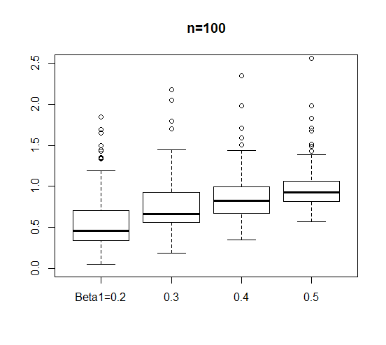
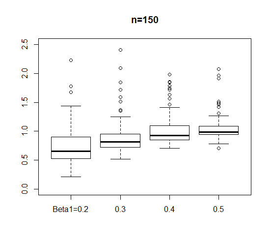
We compare the estimated s^\hat{s} with the true ss in two settings. The first setting has p=200,n=100,s=10,θ=0.02p=200,n=100,s=10,\theta=0.02, and β1=0.2−0.5\beta_{1}=0.2-0.5. The second setting increases sample size nn to 150150. As claimed in Theorem 2.2, the accuracy of s^\hat{s} increases with the magnitude of non-zero coefficients and the sample size. Figure 1 presents the box-plots of the ratio s^/s\hat{s}/s from 100 replications. When β1\beta_{1} or sample size is small, s^\hat{s} tends to under-estimate the true ss. As β1\beta_{1} increases from 0.2 to 0.5 or nn increases from 100 to 150, s^/s\hat{s}/s concentrates more around 1.

Fig 1: Box-plots of s^/s\hat{s}/s with p=200,s=10p=200,s=10, and β1\beta_{1} increasing from 0.20.2 to 0.50.5. The left plot has n=100n=100 and the right plot has n=150n=150.
Refer to caption
Refer to caption

4.2 FNP control

We apply the FNC-Reg algorithm presented in Section 3.2 to the simulated data with p=200p=200, n=150n=150, s=10s=10, θ=0.02\theta=0.02, and β1=0.2−0.5\beta_{1}=0.2-0.5. Table 1 has ϵ\epsilon fixed at 0.1 and reports the mean value of 𝖥𝖭𝖯⁡(t∗)\mathsf{FNP}(t^{*}) as β1\beta_{1} increased from 0.2 to 0.5. We also calculated the associated false discovery proportion (𝖥𝖣𝖯⁡(t∗)=𝖥𝖯⁡(t∗)/R⁡(t∗)\mathsf{FDP}(t^{\ast})=\mathsf{FP}(t^{\ast})/R(t^{\ast})) to reveal the price in incurring false positives for FNP control. Further, we calculate the F-measure, which summarizes FNP and FDP by the harmonic mean of (1-FNP) and (1-FDP) [30]. F-measure takes a value between 0 and 1, and higher value corresponds to better summarized performance.

Because we are not aware of any existing methods that directly control FNP in high-dimensional regression, we present the corresponding results of two other methods that perform variable selection based on different criteria. These results help to better understand the results of FNC-Reg. The first method is Lasso whose solution is obtained using the R package hdi, in which λ\lambda is determined by cross validation. The second method is Knockoff, which has been developed to control false discovery rate (FDR) at a user-specified level in high-dimensional regression [3, 9]. We use the ”knockoff.filter” function in default from the R package knockoff, which creates model-X second-order Gaussian knockoffs as introduced in [9]. The nominal level is set at 0.1.

Table 1: The mean values and standard deviations (in brackets) of FNP, FDP, and the F-measure from 100 replications for FNC-Reg, Lasso, and Knockoff.
β1\beta_{1} Method FNP FDP F-measure
0.20.2 FNC-Reg 0.37 (0.16) 0.35 (0.30) 0.58 (0.20)
Lasso 0.29 (0.12) 0.51 (0.16) 0.56 (0.16)
Knockoff 0.91 (0.23) 0.06 (0.16) 0.08 (0.21)
0.30.3 FNC-Reg 0.19 (0.11) 0.20 (0.24) 0.77 (0.17)
Lasso 0.15 (0.09) 0.43 (0.11) 0.67 (0.09)
Knockoff 0.60 (0.44) 0.11 (0.15) 0.37 (0.41)
0.40.4 FNC-Reg 0.10 (0.09) 0.17 (0.25) 0.84 (0.19)
Lasso 0.06 (0.07) 0.42 (0.12) 0.71 (0.10)
Knockoff 0.34 (0.45) 0.12 (0.14) 0.61 (0.42)
0.50.5 FNC-Reg 0.04 (0.09) 0.13 (0.22) 0.90 (0.18)
Lasso 0.02 (0.10) 0.38 (0.12) 0.74 (0.14)
Knockoff 0.21 (0.49) 0.09 (0.11) 0.74 (0.38)

It can be seen from Table 1 that as β1\beta_{1} increases, the FNP of FNC-Reg decreases, which agrees with the theoretical insight provided by the condition on μm​i​n\mu_{min} in Theorem 3.1. In the challenging scenarios where β1\beta_{1} is very small, the FNP of FNC-Reg mostly exceeds the nominal level of 0.1, which is due to the under-estimation of s^\hat{s} and FNC-Reg’s tendency to select less variables to capture the under-estimated number of signals. Furthermore, both FNP and FDP of FNC-Reg get smaller for larger β1\beta_{1}, suggesting that FNC-Reg automatically adapt to and benefit from increasing signal intensity for both false negative and false positive control. Table 1 also shows that Lasso has lower FNP and much higher FDP than FNC-Reg, which agrees with Lasso’s known tendency of over-selection when p>np>n. On the other hand, Knockoff has FDP reasonably controlled at the nominal level of 0.1 but much higher FNP than those of FNC-Reg and Lasso. In terms of the F-measure that summarizes FNP and FDP, FNC-Reg seems to outperform the other two methods under different β1\beta_{1} values.

We further illustrate the adaptivity of FNC-Reg to the user-specified control level of FNP. For various values of ϵ\epsilon, we calculate the relative frequency of the event {𝖥𝖭𝖯(t∗(ϵ))≤ϵ}\left\{\mathsf{FNP}(t^{\ast}(\epsilon))\leq\epsilon\right\}. Table 2 summarizes the results for different settings with ϵ=0.1,0.2,0.3\epsilon=0.1,0.2,0.3 and β1=0.3,0.5,0.7\beta_{1}=0.3,0.5,0.7. It can be seen that the relative frequency of 𝖥𝖭𝖯≤ϵ\mathsf{FNP}\leq\epsilon for FNC-Reg increases with β1\beta_{1}, which is consistent with the theoretical insight in Theorem 3.1. On the other hand, for a fixed β1\beta_{1}, the relative frequency of 𝖥𝖭𝖯≤ϵ\mathsf{FNP}\leq\epsilon and the FDP of FNC-Reg decreases with ϵ\epsilon, which agrees with our expectation for FNC-Reg as more liberal control of FNP incurs less price in false positives. Note that the results of Lasso and Knockoff do not change with the varying ϵ\epsilon.

Table 2: The relative frequencies of the event {𝖥𝖭𝖯<ϵ}\{\mathsf{FNP}<\epsilon\} and mean values of FDP from 100 replications for FNC-Reg.
β1=0.3\beta_{1}=0.3 β1=0.5\beta_{1}=0.5 β1=0.7\beta_{1}=0.7
ϵ=0.1\epsilon=0.1 0.20.2 0.30.3 ϵ=0.1\epsilon=0.1 0.20.2 0.30.3 ϵ=0.1\epsilon=0.1 0.20.2 0.30.3
1​(𝖥𝖭𝖯≤ϵ)1(\mathsf{FNP}\leq\epsilon) 0.38 0.53 0.71 0.72 0.86 0.91 0.98 0.98 0.98
FDP 0.20 0.15 0.09 0.13 0.08 0.05 0.14 0.10 0.07

5 Conclusion and Discussion

We propose a new variable selection method, FNC-Reg, to efficiently control false negatives in linear regression. Different from existing methods and theory for power analysis and Sure Screening, our procedure directly estimates the FNP of a decision rule and selects the smallest subset of variables that has the estimated FNP less than a user-specified control level. FNP control is specifically challenging when relevant variables cannot be consistently separated from irrelevant ones due to limited sample size and effect size. We develop new techniques to analyze FNP control in the challenging setting and to cope with difficulties caused by the dependence of test statistics.

FNC-Reg possesses two types of adaptivity property. First, it adapts to the user’s preference level on the control of FNP. When a user can tolerate a less stringent control on FNP, he or she can input a larger ϵ\epsilon in the FNC-Reg procedure and select less variables with less false positives. Secondly, the proposed method is adaptive to the unknown effect size. Note that the implementation of the procedure does not requires the information of effect size. Nevertheless, the result of the procedure automatically improves in both FNP and FDP as effect size increases.

Our theoretical study presents a weaker condition on μm​i​n\mu_{min} for FNP control by FNC-Reg than the beta-min condition for variable selection consistency. It is also of interest to understand the result of FNC-Reg if the condition on μmin\mu_{\min} may not be satisfied. Assume that among the ss signal variables only s1s_{1} of them satisfy μj≥2​(γ∗+c)​log⁡p\mu_{j}\geq\sqrt{2(\gamma^{*}+c)\log p} for some constant c>0c>0. Then, similar arguments as in the proof of Theorem 2.2 can be applied to show that P⁡((1−δ)​s1<s^<(1+δ)​s)→1P((1-\delta)s_{1}<\hat{s}<(1+\delta)s)\to 1 for any δ>0\delta>0. Note that s^\hat{s} does not consistently estimate ss anymore, nor is it a consistent estimator for s1s_{1}. Such s^\hat{s} tends to under-estimate ss, which can cause the proposed method to select less variables to capture the under-estimated number of signals. Because FNC-Reg ranks the test statistics by their significance and select variables from the top, one can make a statement about FNP control for the signals with effect sizes larger than the observed cut-off position. Such interpretation of results remains valid whether the condition on μm​i​n\mu_{min} holds or not.

Last but not least, we adopt the debiased Lasso estimator as the test statistic in the paper to demonstrate the new analytic framework of FNP control. We expect that the proposed framework can incorporate other test statistics in linear regression and promote further developments in false negative control based variable selection.

6 Proofs

This section contains the proofs of Theorem 2.1, Theorem 2.2, and Theorem 3.1. Auxiliary lemmas are provided in the appendices. We will frequently use the Mill’s ratio, i.e.,

Φ¯​(x)=x−1​ϕ​(x)​(1+o⁡(1))​ for ​x→+∞,\bar{\Phi}\left(x\right)={x}^{-1}\phi\left(x\right)\left(1+o\left(1\right)\right)\text{ \ for \ }x\rightarrow+\infty,

without mentioning it at each instance. All arguments will be conditional on 𝐗\mathbf{X}, and the symbol CC denotes a generic, finite constant whose values can be different at different occurrences.

6.1 Proof of Theorem 2.1

The proof is composed of two parts. The first part assumes ξ>η\xi>\eta and the second part assumes ξ≤η\xi\leq\eta.

Consider the first part with ξ>η\xi>\eta. It suffices to show s−1​𝖥𝖯​(tξ)=oP​(1)s^{-1}\mathsf{FP}\left(t_{\xi}\right)=o_{P}(1) and s−1​p0​Φ​(−tξ)=o⁡(1)s^{-1}p_{0}\Phi\left(-t_{\xi}\right)=o(1) with ξ>η\xi>\eta. By Mill’s ratio,

s−1​p​Φ​(−tξ)≤C​pη−ξ/log⁡p=o⁡(1)s^{-1}p\Phi\left(-t_{\xi}\right)\leq Cp^{\eta-\xi}/\sqrt{\log p}=o(1)

when ξ>η\xi>\eta. On the other hand, for a fixed constant a>0a>0,

P⁡(s−1​𝖥𝖯​(tξ)>a)≤E⁡(𝖥𝖯⁡(tξ))a​s=p0​maxj∈I0⁡P⁡(|zj|>tξ)a​s.P\left(s^{-1}\mathsf{FP}\left(t_{\xi}\right)>a\right)\leq\frac{E\left(\mathsf{FP}\left(t_{\xi}\right)\right)}{as}=\frac{p_{0}\max_{j\in I_{0}}P\left(\left|z_{j}\right|>t_{\xi}\right)}{as}.

The following lemma help quantify the order of P⁡(|zj|>tξ)P(|z_{j}|>t_{\xi}) for j∈I0j\in I_{0}, and its proof is provided in Section A.3.

Lemma 6.1.

Assume A1) through A3). Define

dp=C1​(s​log​p/n+min⁡{s,sm​a​x}​log​p/n)d_{p}=C_{1}\left(\sqrt{s}\log p/\sqrt{n}+\min\left\{s,s_{max}\right\}\log p/\sqrt{n}\right)

for some constant C1≥max⁡{1,2​(σ​Cmin)−1}C_{1}\geq\max\left\{1,2(\sigma\sqrt{C_{\min}})^{-1}\right\}. Then

|P⁡(|wj′−δj′|>tξ)−P⁡(|wj′|>tξ)|≤C​p−ξ​dp+C​p−2.\left|P(|w^{\prime}_{j}-\delta^{\prime}_{j}|>t_{\xi})-P(|w^{\prime}_{j}|>t_{\xi})\right|\leq Cp^{-\xi}d_{p}+Cp^{-2}.

Recall s=p1−ηs=p^{1-\eta} with 0<η<10<\eta<1. Then Lemma 6.1 implies

P⁡(s−1​𝖥𝖯​(tξ)>a)≤C​p0​(p−ξ+p−ξ​dp+p−2)p1−η=o⁡(1),P\left(s^{-1}\mathsf{FP}\left(t_{\xi}\right)>a\right)\leq\frac{Cp_{0}\left(p^{-\xi}+p^{-\xi}d_{p}+p^{-2}\right)}{p^{1-\eta}}=o\left(1\right),

where the last step is by dp=o⁡(1)d_{p}=o(1) under A3) and ξ>η\xi>\eta. Then s−1​𝖥𝖯​(tξ)=oP​(1)s^{-1}\mathsf{FP}\left(t_{\xi}\right)=o_{P}\left(1\right). This justifies the claim of Theorem 2.1 for ξ>η\xi>\eta.

Next, we present the second part of the proof with ξ≤η\xi\leq\eta. Define

Dp=s−2​(p1−ξ+p2−ξ​λ1​sm​a​x)​log⁡p.D_{p}=s^{-2}(p^{1-\xi}+p^{2-\xi}\lambda_{1}\sqrt{s_{max}})\log p.

By the order of λ1\lambda_{1} in A2) and condition ξ>γ1∗\xi>\gamma^{*}_{1}, Dp=o⁡(1)D_{p}=o(1). Then it is sufficient to show

P⁡(s−1​|𝖥𝖯⁡(tξ)−2​p0​Φ​(−tξ)|>Dp)→0.P(s^{-1}\left|\mathsf{FP}(t_{\xi})-2p_{0}\Phi(-t_{\xi})\right|>\sqrt{D_{p}})\to 0.

Perform the decomposition

s−1​|𝖥𝖯⁡(tξ)−2​p0​Φ​(−tξ)|\displaystyle s^{-1}\left|\mathsf{FP}(t_{\xi})-2p_{0}\Phi(-t_{\xi})\right| ≤\displaystyle\leq s−1​|𝖥𝖯⁡(tξ)−𝖤⁡(𝖥𝖯⁡(tξ))|\displaystyle s^{-1}\left|\mathsf{FP}(t_{\xi})-\mathsf{E}(\mathsf{FP}(t_{\xi}))\right|
+\displaystyle+ s−1​|𝖤⁡(𝖥𝖯⁡(tξ)−2​p0​Φ​(−tξ))|.\displaystyle s^{-1}\left|\mathsf{E}(\mathsf{FP}(t_{\xi})-2p_{0}\Phi(-t_{\xi}))\right|.

Then it is sufficient to show

s−1​|𝖥𝖯⁡(tξ)−𝖤⁡(𝖥𝖯⁡(tξ))|=op​(Dp)s^{-1}\left|\mathsf{FP}(t_{\xi})-\mathsf{E}(\mathsf{FP}(t_{\xi}))\right|=o_{p}(\sqrt{D_{p}}) (6.1)

and

s−1​|𝖤⁡(𝖥𝖯⁡(tξ)−2​p0​Φ​(−tξ))|=o⁡(Dp).s^{-1}\left|\mathsf{E}(\mathsf{FP}(t_{\xi})-2p_{0}\Phi(-t_{\xi}))\right|=o(\sqrt{D_{p}}). (6.2)

Consider (6.1) first. By Chebyshev’s inequality,

P⁡(s−1​|𝖥𝖯⁡(tξ)−𝖤⁡(𝖥𝖯⁡(tξ))|>Dp)≤𝖵𝖺𝗋⁡(𝖥𝖯⁡(tξ))s2​Dp.P(s^{-1}\left|\mathsf{FP}(t_{\xi})-\mathsf{E}(\mathsf{FP}(t_{\xi}))\right|>\sqrt{D_{p}})\leq{\mathsf{Var}(\mathsf{FP}(t_{\xi}))\over s^{2}D_{p}}.

We derive the order of 𝖵𝖺𝗋⁡(𝖥𝖯⁡(tξ))\mathsf{Var}(\mathsf{FP}(t_{\xi})). By Lemma 6.1, P⁡(|wj′−δj′|>tξ)=P⁡(|wj′|>tξ)​(1+o⁡(1))P(|w^{\prime}_{j}-\delta^{\prime}_{j}|>t_{\xi})=P(|w^{\prime}_{j}|>t_{\xi})(1+o(1)) given dp=o⁡(1/log⁡p)d_{p}=o(1/\sqrt{\log p}) from A3) and ξ≤η<1\xi\leq\eta<1, then direct calculation gives

𝖵𝖺𝗋⁡(𝖥𝖯⁡(tξ))=𝖵𝖺𝗋⁡(𝖥𝖯w′​(tξ))​(1+o⁡(1)),\mathsf{Var}(\mathsf{FP}(t_{\xi}))=\mathsf{Var}(\mathsf{FP}_{w^{\prime}}(t_{\xi}))(1+o(1)),

where 𝖥𝖯w′(tξ)=∑j∈I01{|wj′|>tξ}\mathsf{FP}_{w^{\prime}}(t_{\xi})=\sum\nolimits_{j\in I_{0}}1_{\{|w_{j}^{\prime}|>t_{\xi}\}}. The following lemma is proved in Section A.4.

Lemma 6.2.

Assume A1) and A2) and let tξ=2​ξ​log⁡pt_{\xi}=\sqrt{2\xi\log p} for any ξ>0\xi>0. Then

𝖵𝖺𝗋(∑j=1p1{|wj′|>tξ})=O(p1−ξ+p2−ξλ1sm​a​x).\mathsf{Var}\left(\sum\nolimits_{j=1}^{p}1_{\{|w_{j}^{\prime}|>t_{\xi}\}}\right)=O\left(p^{1-\xi}+p^{2-\xi}\lambda_{1}\sqrt{s_{max}}\right).

The above gives

𝖵𝖺𝗋⁡(𝖥𝖯⁡(tξ))s2​Dp=𝖵𝖺𝗋⁡(𝖥𝖯w′​(tξ))s2​Dp​(1+o⁡(1))=o⁡(1),{\mathsf{Var}(\mathsf{FP}(t_{\xi}))\over s^{2}D_{p}}={\mathsf{Var}(\mathsf{FP}_{w^{\prime}}(t_{\xi}))\over s^{2}D_{p}}(1+o(1))=o(1),

so that

P⁡(s−1​|𝖥𝖯⁡(tξ)−𝖤⁡(𝖥𝖯⁡(tξ))|>Dp)→0.P(s^{-1}\left|\mathsf{FP}(t_{\xi})-\mathsf{E}(\mathsf{FP}(t_{\xi}))\right|>\sqrt{D_{p}})\to 0.

Next consider (6.2). By Lemma 6.1

s−1​|𝖤⁡(𝖥𝖯⁡(tξ)−2​p0​Φ​(−tξ))|\displaystyle s^{-1}\left|\mathsf{E}(\mathsf{FP}(t_{\xi})-2p_{0}\Phi(-t_{\xi}))\right| ≤\displaystyle\leq s−1​∑j∈I0|P⁡(|wj′−δj′|>tξ)−P⁡(|wj′|>tξ)|\displaystyle s^{-1}\sum_{j\in I_{0}}\left|P(|w^{\prime}_{j}-\delta^{\prime}_{j}|>t_{\xi})-P(|w^{\prime}_{j}|>t_{\xi})\right|
≤\displaystyle\leq C​s−1​p1−ξ​dp+C​s−1​p−1.\displaystyle Cs^{-1}p^{1-\xi}d_{p}+Cs^{-1}p^{-1}.

Recall s=p1−ηs=p^{1-\eta} and the definitions of dpd_{p} and DpD_{p}. Note that dp>s​log⁡p/nd_{p}>s\log p/\sqrt{n}, then direct calculation gives

s−1​p1−ξ​dp=o⁡(Dp)s^{-1}p^{1-\xi}d_{p}=o(\sqrt{D_{p}})

under condition ξ>γ2∗\xi>\gamma^{*}_{2}, and

s−1​p−1=o⁡(Dp)s^{-1}p^{-1}=o(\sqrt{D_{p}})

with ξ≤η<1\xi\leq\eta<1. (6.2) follows consequently. This concludes the second part of the proof with ξ≤η\xi\leq\eta.

6.2 Proof of Theorem 2.2

First, we have the following lemma showing the order of the bounding sequence cp∗c_{p}^{\ast} for Vp∗V_{p}^{\ast}. The proof is provided in Section A.5.

Lemma 6.3.

Assume conditions A1) through A3) in Appendix A.1. Consider Vp∗V_{p}^{\ast} as in (2.15). Then cp∗c_{p}^{\ast} at the order of (sm​a​x/n)1/4​log⁡p(s_{max}/n)^{1/4}\log p satisfies P⁡(Vp∗>cp∗)→0P(V_{p}^{\ast}>c_{p}^{\ast})\rightarrow 0 as p→∞p\rightarrow\infty.

Now, recall Fp(t)=p−1∑j=1p1{|zj|>t}F_{p}(t)=p^{-1}\sum_{j=1}^{p}1_{\{|z_{j}|>t\}} and define Φ¯p(t)=p−1∑j=1p1{|μj+wj′|>t}\bar{\Phi}_{p}(t)=p^{-1}\sum_{j=1}^{p}1_{\{|\mu_{j}+w_{j}^{\prime}|>t\}}. Consider the decomposition

π^∗=maxt∈𝕋⁡{Fp​(t)−Φ¯p​(t)1−2​Φ¯​(t)+Φ¯p​(t)−2​Φ¯​(t)−cp∗​σ¯​(t)1−2​Φ¯​(t)},\hat{\pi}^{\ast}=\max_{t\in\mathbb{T}}\left\{{\frac{F_{p}(t)-\bar{\Phi}_{p}(t)}{1-2\bar{\Phi}(t)}}+\frac{\bar{\Phi}_{p}(t)-2\bar{\Phi}(t)-c_{p}^{\ast}\bar{\sigma}\left(t\right)}{1-2\bar{\Phi}(t)}\right\}, (6.3)

where 𝕋\mathbb{T} is defined in (A.10). The first summand within the parentheses on the right hand side (RHS) of (6.3) can be safely ignored when bounding π^∗/π\hat{\pi}^{\ast}/\pi as asserted by the following Lemma 6.4.

Lemma 6.4.

Assume t=tξ=2​ξ​log⁡pt=t_{\xi}=\sqrt{2\xi\log p} with ξ>γ∗\xi>\gamma^{*}. Then

π−1​|Fp​(t)−Φ¯p​(t)|​(1−2​Φ¯​(t))−1=oP​(1).\pi^{-1}\left|F_{p}(t)-\bar{\Phi}_{p}(t)\right|\left(1-2\bar{\Phi}(t)\right)^{-1}=o_{P}(1).

Define

π^∗⁣∗=maxt∈𝕋⁡Φ¯p​(t)−2​Φ¯​(t)−cp∗​σ¯​(t)1−2​Φ¯​(t).\hat{\pi}^{\ast\ast}=\max_{t\in\mathbb{T}}\frac{\bar{\Phi}_{p}(t)-2\bar{\Phi}(t)-c_{p}^{\ast}\bar{\sigma}\left(t\right)}{1-2\bar{\Phi}(t)}.

Then it suffices to show

P⁡(1−δ<π^∗⁣∗/π<1)→1.P(1-\delta<\hat{\pi}^{\ast\ast}/\pi<1)\rightarrow 1. (6.4)

We first show that π^∗⁣∗\hat{\pi}^{\ast\ast} is an asymptotic lower bound of π\pi. Recall the definition of Vp∗V_{p}^{\ast} as

Vp∗=maxt∈𝕋⁡p−1∑j=1p1{|wj′|>t}−2Φ¯(t)σ¯​(t).V_{p}^{\ast}=\max_{t\in\mathbb{T}}\frac{p^{-1}\sum\nolimits_{j=1}^{p}1_{\{|w_{j}^{\prime}|>t\}}-2\bar{\Phi}(t)}{\bar{\sigma}(t)}.

Since

Φ¯p(t)≤p−1s+p−1∑j∈I01{|wj′|>t}=π+(1−π)p0−1∑j∈I01{|wj′|>t},\bar{\Phi}_{p}(t)\leq p^{-1}s+p^{-1}\sum_{j\in I_{0}}1_{\{|w_{j}^{\prime}|>t\}}=\pi+(1-\pi)p_{0}^{-1}\sum_{j\in I_{0}}1_{\{|w_{j}^{\prime}|>t\}},

then

P⁡(π^∗⁣∗>π)\displaystyle P(\hat{\pi}^{\ast\ast}>\pi) ≤\displaystyle\leq P(maxt∈𝕋{(1−π)(p0−1∑j∈I01{|wj′|>t}−2Φ¯(t))−cp∗σ¯(t)}>0)\displaystyle P\left(\max_{t\in\mathbb{T}}\left\{(1-\pi)\left(p_{0}^{-1}\sum\nolimits_{j\in I_{0}}1_{\{|w_{j}^{\prime}|>t\}}-2\bar{\Phi}(t)\right)-c_{p}^{\ast}\bar{\sigma}(t)\right\}>0\right)
≤\displaystyle\leq P(maxt∈𝕋{p0−1∑j∈I01{|wj′|>t}−2Φ¯(t)−cp0∗σ¯(t)}>0)\displaystyle P\left(\max_{t\in\mathbb{T}}\left\{p_{0}^{-1}\sum\nolimits_{j\in I_{0}}1_{\{|w_{j}^{\prime}|>t\}}-2\bar{\Phi}(t)-c_{p_{0}}^{\ast}\bar{\sigma}(t)\right\}>0\right)
≤\displaystyle\leq P⁡(Vp0∗>cp0∗),\displaystyle P\left(V_{p_{0}}^{\ast}>c_{p_{0}}^{\ast}\right),

where the second inequality follows since cp∗c_{p}^{\ast} is non-decreasing in pp and cp∗​(1−π)−1>cp0∗c_{p}^{\ast}(1-\pi)^{-1}>c_{p_{0}}^{\ast}. However, Lemma 6.3 asserts P⁡(Vp0∗>cp0∗)→0P(V_{p_{0}}^{\ast}>c_{p_{0}}^{\ast})\rightarrow 0. So,

P⁡(π^∗⁣∗>π)≤P⁡(Vp0∗>cp0∗)→0.P(\hat{\pi}^{\ast\ast}>\pi)\leq P(V_{p_{0}}^{\ast}>c_{p_{0}}^{\ast})\rightarrow 0. (6.5)

Next, we show that π^∗⁣∗\hat{\pi}^{\ast\ast} is an asymptotic upper bound of (1−δ)​π(1-\delta)\pi for any δ>0\delta>0. Let 𝖥𝖯w′(t)=∑j∈I01{|wj′|>t}\mathsf{FP}_{w^{\prime}}(t)=\sum\nolimits_{j\in I_{0}}1_{\{|w_{j}^{\prime}|>t\}} and rewrite

Φ¯p(t)=πs∑j∈I11{|μj+wj′|>t}+1−πp0𝖥𝖯w′(t).\bar{\Phi}_{p}(t)={\frac{\pi}{s}}\sum_{j\in I_{1}}1_{\{|\mu_{j}+w_{j}^{\prime}|>t\}}+{\frac{1-\pi}{p_{0}}}\mathsf{FP}_{w^{\prime}}(t).

Since π^∗⁣∗>Φ¯p​(t)−2​Φ¯​(t)−cp∗​σ¯​(t)\hat{\pi}^{\ast\ast}>\bar{\Phi}_{p}(t)-2\bar{\Phi}(t)-c_{p}^{\ast}\bar{\sigma}\left(t\right) for any t∈𝕋t\in\mathbb{T}, then

π^∗⁣∗π−1\displaystyle\frac{\hat{\pi}^{\ast\ast}}{\pi}-1 >\displaystyle> (s−1∑j∈I11{|μj+wj′|>t}−1)−2Φ¯(t)\displaystyle\left({s}^{-1}\sum\nolimits_{j\in I_{1}}1_{\{|\mu_{j}+w_{j}^{\prime}|>t\}}-1\right)-2\bar{\Phi}(t) (6.6)
+1−ππ​(p0−1​𝖥𝖯w′​(t)−2​Φ¯​(t))−1π​cp∗​σ¯​(t)\displaystyle+\frac{1-\pi}{\pi}\left(p_{0}^{-1}\mathsf{FP}_{w^{\prime}}(t)-2\bar{\Phi}(t)\right)-\frac{1}{\pi}c_{p}^{\ast}\bar{\sigma}(t)

for any any t∈𝕋t\in\mathbb{T}. Now set tt in the inequality (6.6) to be

tτ=2​τ​log⁡p​ with ​τ=γ∗+c/2,t_{\tau}=\sqrt{2\tau\log p}\text{ \ with }\tau=\gamma^{\ast}+c/2, (6.7)

where γ∗\gamma^{\ast} is defined in (2.11). We will show that each term on the RHS of (6.6) is oP​(1)o_{P}\left(1\right).

Firstly, cp∗=O⁡((sm​a​x/n)1/4​log⁡p)c_{p}^{\ast}=O\left(\left(s_{max}/n\right)^{1/4}\log p\right) set in Lemma 6.3 implies the last term at tτt_{\tau}

π−1​cp∗​σ¯​(tτ)=O⁡(pη−τ/2​(sm​a​x/n)1/4​log⁡p)=o⁡(1).\pi^{-1}c_{p}^{\ast}\bar{\sigma}(t_{\tau})=O(p^{\eta-\tau/2}(s_{max}/n)^{1/4}\log p)=o(1).

The second term 2​Φ¯​(tτ)=O⁡(p−τ/log⁡p)=o⁡(1)2\bar{\Phi}(t_{\tau})=O(p^{-\tau}/\sqrt{\log p})=o(1).

Consider the third term at tτt_{\tau}. Similar arguments for (2.12) can be applied to show s−1​|𝖥𝖯w′​(tτ)−2​p0​Φ¯​(tτ)|=oP​(1)s^{-1}|\mathsf{FP}_{w^{\prime}}(t_{\tau})-2p_{0}\bar{\Phi}(t_{\tau})|=o_{P}(1). Then

1−ππ​|p0−1​𝖥𝖯w′​(t)−2​Φ¯​(t)|≤C​s−1​|𝖥𝖯w′​(tτ)−2​p0​Φ¯​(tτ)|=oP​(1).\frac{1-\pi}{\pi}\left|p_{0}^{-1}\mathsf{FP}_{w^{\prime}}(t)-2\bar{\Phi}(t)\right|\leq Cs^{-1}|\mathsf{FP}_{w^{\prime}}(t_{\tau})-2p_{0}\bar{\Phi}(t_{\tau})|=o_{P}(1).

For the first term of (6.6), let A1​(t)=A_{1}\left(t\right)= s−1∑j∈I11{|μj+wj′|≤t}{s}^{-1}\sum\nolimits_{j\in I_{1}}1_{\{|\mu_{j}+w_{j}^{\prime}|\leq t\}}. Then the first term is s−1∑j∈I11{|μj+wj′|>tτ}−1=A1(tτ){s}^{-1}\sum\nolimits_{j\in I_{1}}1_{\{|\mu_{j}+w_{j}^{\prime}|>t_{\tau}\}}-1=A_{1}\left(t_{\tau}\right). The following lemma shows A1​(tτ)=oP​(1)A_{1}\left(t_{\tau}\right)=o_{P}\left(1\right), and its proof is provided in Section A.7.

Lemma 6.5.

Let A1​(t)=A_{1}\left(t\right)= s−1∑j∈I11{|μj+wj′|≤t}{s}^{-1}\sum\nolimits_{j\in I_{1}}1_{\{|\mu_{j}+w_{j}^{\prime}|\leq t\}} and assume μm​i​n≥2​(γ∗+c)​log⁡p\mu_{min}\geq\sqrt{2(\gamma^{\ast}+c)\log p}. Then A1​(tτ)=oP​(1)A_{1}\left(t_{\tau}\right)=o_{P}\left(1\right) for tτt_{\tau} in (6.7).

Thus, we have shown

P⁡(π^∗⁣∗/π−1<−δ)→0P(\hat{\pi}^{\ast\ast}/\pi-1<-\delta)\rightarrow 0 (6.8)

for any δ>0\delta>0. Consequently, (6.4) follows from (6.5) and (6.8).

6.3 Proof of Theorem 3.1

Recall 𝖥𝖭𝖯⁡(t)=1−s−1​R​(t)+s−1​F​P​(−t)\mathsf{FNP}\left(t\right)=1-s^{-1}R\left(t\right)+s^{-1}FP\left(-t\right) and 𝖥𝖭𝖯^​(t)=1−s^−1​R​(t)+2​s^−1​p​Φ​(−t)\widehat{\mathsf{FNP}}\left(t\right)=1-\hat{s}^{-1}R\left(t\right)+2\hat{s}^{-1}p\Phi\left(-t\right) for t≥0t\geq 0. Recall the definition of t∗​(ϵ)t^{*}(\epsilon) and simplify the notation by t∗=t∗​(ϵ)t^{*}=t^{*}(\epsilon). We have the following Lemma 6.6, whose proof is provided in Section A.8.

Lemma 6.6.

Assume μm​i​n≥2​(γ∗+c)​log⁡p\mu_{min}\geq\sqrt{2(\gamma^{\ast}+c)\log p}. If t∗t^{*} satisfies P⁡(t∗≥tτ)→1P\left(t^{\ast}\geq t_{\tau}\right)\rightarrow 1 for tτt_{\tau} in (6.7), then

|𝖥𝖭𝖯^​(t∗)−𝖥𝖭𝖯⁡(t∗)|=oP​(1).|\widehat{\mathsf{FNP}}(t^{\ast})-\mathsf{FNP}(t^{\ast})|=o_{P}(1). (6.9)

Now we aim to show P⁡(t∗≥tτ)→1P\left(t^{\ast}\geq t_{\tau}\right)\rightarrow 1. The proof of the following Lemma 6.7 is presented in Section A.9.

Lemma 6.7.

Assume μm​i​n≥2​(γ∗+c)​log⁡p\mu_{min}\geq\sqrt{2(\gamma^{\ast}+c)\log p}. Then, for tτt_{\tau} in (6.7),

𝖥𝖭𝖯⁡(tτ)=oP​(1).\mathsf{FNP}(t_{\tau})=o_{P}\left(1\right). (6.10)

Note that a special case of (6.9) is |𝖥𝖭𝖯^​(tτ)−𝖥𝖭𝖯⁡(tτ)|=oP​(1)|\widehat{\mathsf{FNP}}(t_{\tau})-\mathsf{FNP}(t_{\tau})|=o_{P}(1), which holds when t∗t^{\ast} is set to be tτt_{\tau}. Then (6.10) implies 𝖥𝖭𝖯^​(tτ)=oP​(1)\widehat{\mathsf{FNP}}(t_{\tau})=o_{P}\left(1\right), and P⁡(t∗≥tτ)→1P\left(t^{\ast}\geq t_{\tau}\right)\rightarrow 1 follows from the definition of t∗t^{\ast}.

On the other hand, the definition of t∗t^{*} implies 𝖥𝖭𝖯^​(t∗)<ϵ\widehat{\mathsf{FNP}}(t^{\ast})<\epsilon almost surely, then Lemma 6.6 implies P⁡(𝖥𝖭𝖯⁡(t∗)<ϵ)→1P(\mathsf{FNP}(t^{\ast})<\epsilon)\rightarrow 1 as stated in (3.2).

Next, we show (3.3). Denote

𝖥𝖭𝖯^π^​(t)=1−R⁡(t)−2​p​Φ​(−t)π^​pand𝖥𝖭𝖯^π^∗​(t)=1−R⁡(t)−2​p​Φ​(−t)π^∗​p.\widehat{\mathsf{FNP}}_{\hat{\pi}}(t)=1-\frac{R\left(t\right)-2p\Phi\left(-t\right)}{\hat{\pi}p}\qquad\text{and}\qquad\widehat{\mathsf{FNP}}_{\hat{\pi}^{*}}(t)=1-\frac{R\left(t\right)-2p\Phi\left(-t\right)}{\hat{\pi}^{*}p}.

By the definition of π^\hat{\pi} and π^∗\hat{\pi}^{*} and cp=cp∗c_{p}=c_{p}^{*}, it is easy to see that π^≥π^∗\hat{\pi}\geq\hat{\pi}^{*} and, consequently,

𝖥𝖭𝖯^π^​(t)≥𝖥𝖭𝖯^π^∗​(t)\widehat{\mathsf{FNP}}_{\hat{\pi}}(t)\geq\widehat{\mathsf{FNP}}_{\hat{\pi}^{*}}(t)

for any t>0t>0. Denote

tπ^∗=sup{t:𝖥𝖭𝖯^π^​(t)≤ϵ}andtπ^∗∗=sup{t:𝖥𝖭𝖯^π^∗​(t)≤ϵ}.t^{\ast}_{\hat{\pi}}=\sup\left\{t:\widehat{\mathsf{FNP}}_{\hat{\pi}}(t)\leq\epsilon\right\}\qquad\text{and}\qquad t^{\ast}_{\hat{\pi}^{*}}=\sup\left\{t:\widehat{\mathsf{FNP}}_{\hat{\pi}^{*}}(t)\leq\epsilon\right\}.

Then tπ^∗≤tπ^∗∗t^{*}_{\hat{\pi}}\leq t^{*}_{\hat{\pi}^{*}} almost surely.

Recall 𝖥𝖭𝖯⁡(tπ^∗∗)<ϵ\mathsf{FNP}(t^{*}_{\hat{\pi}^{*}})<\epsilon with probability tending to 1 as stated in (3.2) and the fact that 𝖥𝖭𝖯⁡(t)\mathsf{FNP}(t) is non-decreasing in tt, then 𝖥𝖭𝖯⁡(tπ^∗)≤𝖥𝖭𝖯⁡(tπ^∗∗)<ϵ\mathsf{FNP}(t^{*}_{\hat{\pi}})\leq\mathsf{FNP}(t^{*}_{\hat{\pi}^{*}})<\epsilon with probability tending to 1. Therefore (3.3) holds.

A Appendix

The notations we will use throughout the appendices are collected as follows. For a matrix 𝐌\mathbf{M}, the qq-norm ‖𝐌‖q=(∑i,j|𝐌i​j|q)1/q\left\|\mathbf{M}\right\|_{q}=\left(\sum_{i,j}\left|\mathbf{M}_{ij}\right|^{q}\right)^{1/q} for q>0q>0, ∞\infty-norm ‖𝐌‖∞=maxi,j⁡|𝐌i​j|\left\|\mathbf{M}\right\|_{\infty}=\max_{i,j}\left|\mathbf{M}_{ij}\right|, and ‖𝐌‖1,∞\left\|\mathbf{M}\right\|_{1,\infty} the maximum of the 11-norm of each row of 𝐌\mathbf{M}. If 𝐌\mathbf{M} is symmetric, σi​(𝐌)\sigma_{i}(\mathbf{M}) denotes the iith largest eigenvalue of 𝐌\mathbf{M}.

A.1 Debiased Lasso

The matrix 𝚯^∈ℝp×p\hat{\boldsymbol{\Theta}}\in\mathbb{R}^{p\times p} appearing in the debiased Lasso estimator for 𝜷\boldsymbol{\beta} in the main text is obtained as follows. Let 𝐗−j\mathbf{X}_{-j} denote the matrix obtained by removing the jjth column of 𝐗\mathbf{X}. For each j=1,…,pj=1,\ldots,p, let

𝜸^j=arg⁡min𝜸∈ℝp−1⁡(n−1​‖𝐱j−𝐗−j​𝜸‖22+2​λj​‖𝜸‖1)\hat{\boldsymbol{\gamma}}_{j}=\argmin_{\boldsymbol{\gamma}\in\mathbb{R}^{p-1}}\left(n^{-1}\left\|\mathbf{x}_{j}-\mathbf{X}_{-j}\boldsymbol{\gamma}\right\|_{2}^{2}+2\lambda_{j}\left\|\boldsymbol{\gamma}\right\|_{1}\right) (A.1)

with components γ^j,k,k=1,…,p\hat{\gamma}_{j,k},k=1,\ldots,p and k≠jk\neq j, and define

τ^j2=n−1​‖𝐱j−𝐗−j​𝜸^j‖22+2​λj​‖𝜸^j‖1.\hat{\tau}_{j}^{2}=n^{-1}\left\|\mathbf{x}_{j}-\mathbf{X}_{-j}\hat{\boldsymbol{\gamma}}_{j}\right\|_{2}^{2}+2\lambda_{j}\left\|\hat{\boldsymbol{\gamma}}_{j}\right\|_{1}.

Then

𝚯^=diag​(τ^1−2,⋯,τ^p−2)​(1−γ^1,2⋯−γ^1,p−γ^2,11⋯−γ^2,p⋮⋮⋮⋮−γ^p,1−γ^p,2⋯1).\hat{\boldsymbol{\Theta}}=\text{diag}\left(\hat{\tau}_{1}^{-2},\cdots,\hat{\tau}_{p}^{-2}\right)\left(\begin{array}[]{cccc}1&-\hat{\gamma}_{1,2}&\cdots&-\hat{\gamma}_{1,p}\\ -\hat{\gamma}_{2,1}&1&\cdots&-\hat{\gamma}_{2,p}\\ \vdots&\vdots&\vdots&\vdots\\ -\hat{\gamma}_{p,1}&-\hat{\gamma}_{p,2}&\cdots&1\end{array}\right).

Recall n​(𝐛^−𝜷)=𝐰−𝜹\sqrt{n}(\hat{\mathbf{b}}-\boldsymbol{\beta})=\mathbf{w}-\boldsymbol{\delta}, where 𝐰∼𝒩p​(0,σ2​𝛀^)\mathbf{w}\sim\mathcal{N}_{p}(0,\sigma^{2}\hat{\boldsymbol{\Omega}}) conditional on 𝐗\mathbf{X}. To quantify the magnitude of 𝜹\boldsymbol{\delta}, we adopt and rephrase Theorem 3.13 of [21] for unknown 𝚺\boldsymbol{\Sigma} as follows. Let 𝚯=𝚺−1\boldsymbol{\Theta}=\boldsymbol{\Sigma}^{-1}, sj=|{k≠j:𝚯j​k≠0}|s_{j}=\left|\left\{k\neq j:\boldsymbol{\Theta}_{jk}\neq 0\right\}\right| and sm​a​x=max1≤j≤p⁡sjs_{max}=\max_{1\leq j\leq p}s_{j}.

A1)

Gaussian random design: the rows of 𝐗\mathbf{X} are i.i.d. 𝒩p​(0,𝚺)\mathcal{N}_{p}\left(0,\boldsymbol{\Sigma}\right) for which𝚺\boldsymbol{\ \Sigma} satisfies:

A1a)

max1≤j≤p⁡𝚺j​j≤1\max_{1\leq j\leq p}\boldsymbol{\Sigma}_{jj}\leq 1.

A1b)

0<Cm​i​n≤σ1​(𝚺)≤σp​(𝚺)≤Cm​a​x<∞0<C_{min}\leq\sigma_{1}\left(\boldsymbol{\Sigma}\right)\leq\sigma_{p}\left(\boldsymbol{\Sigma}\right)\leq C_{max}<\infty for constants Cm​i​nC_{min} and Cm​a​x.C_{max}.

A1c)

ρ⁡(Σ,C0​s)≤ρ\rho\left(\Sigma,C_{0}s\right)\leq\rho for some constant ρ>0\rho>0, where C0=32​Cm​a​x​Cm​i​n−1+1C_{0}=32C_{max}C_{min}^{-1}+1,

ρ⁡(𝐀,k)=maxT⊆[p],|T|≤k⁡‖(𝐀T,T)−1‖1,∞\rho\left(\mathbf{A},k\right)=\max_{T\subseteq\left[p\right],\left|T\right|\leq k}\big\|\left(\mathbf{A}_{T,T}\right)^{-1}\big\|_{1,\infty}

for a square matrix 𝐀\mathbf{A}, [p]={1,…,p}\left[p\right]=\left\{1,...,p\right\} , 𝐀T,T\mathbf{A}_{T,T} is a sub-matrix formed by taking entries of 𝐀\mathbf{A} whose row and column indices respectively form the same subset TT.

A2)

Tuning parameters: for the Lasso in (2.1), λ=8​σ​n−1​log⁡p\lambda=8\sigma\sqrt{n^{-1}\log p}; for nodewise regression in (A.1), λj=κ~n−1​log⁡p,j=1,…,p\lambda_{j}=\tilde{\kappa}\sqrt{n^{-1}\log p},j=1,\ldots,p for a suitably large universal constant κ~\tilde{\kappa}.

A3)

Sparsities of 𝜷\boldsymbol{\beta} and 𝚯\boldsymbol{\Theta}: max⁡{s,sm​a​x}=o⁡(n/log⁡p)\max\{s,s_{max}\}=o(n/\log p), min⁡{sm​a​x,s}=o⁡(n/log⁡p)\min\{s_{max},s\}=o(\sqrt{n}/\log p) and s=o⁡(n/(log⁡p)2)s=o\left(n/(\log p)^{2}\right).

Lemma A.1.

Assume A1) and A2). Then there exist positive constants cc and c′c^{\prime} depending only on Cm​i​nC_{min}, Cm​a​xC_{max} and κ~\tilde{\kappa} such that, for max⁡{s,sm​a​x}<c​n/log⁡p\max\{s,s_{max}\}<cn/\log p, the probability that

‖𝜹‖∞≤c′​ρ​σ​sn​log⁡p+c′​σ​min⁡{s,sm​a​x}​log⁡pn\left\|\boldsymbol{\delta}\right\|_{\infty}\leq c^{\prime}\rho\sigma\sqrt{\frac{s}{n}}\log p+c^{\prime}\sigma\min\left\{s,s_{max}\right\}\frac{\log p}{\sqrt{n}} (A.2)

is at least 1−2​p​e−16−1​n​s−1​Cm​i​n−p​e−c​n−6​p−21-2pe^{-16^{-1}ns^{-1}C_{min}}-pe^{-cn}-6p^{-2}. Further, assume A3), then ‖𝛅‖∞=oP​(1)\|\boldsymbol{\delta}\|_{\infty}=o_{P}(1).

Note that the above result relaxed the ultra-sparse condition s=o⁡(n/log⁡p)s=o(\sqrt{n}/\log p) in [34] to s=o⁡(n/(log⁡p)2)s=o\left(n/(\log p)^{2}\right) as shown in A3).

Recall the standardized debiased Lasso estimate zj=nb^jσ−1𝛀^j​j−1/2z_{j}=\sqrt{n}\hat{b}_{j}\sigma^{-1}\hat{\boldsymbol{\Omega}}_{jj}^{-1/2} for 1≤j≤p1\leq j\leq p. Namely, zj=μj+wj′−δj′z_{j}=\mu_{j}+w_{j}^{\prime}-\delta_{j}^{\prime}, wj′=wjσ​𝛀^j​j∼𝒩⁡(0,1)w_{j}^{\prime}=\frac{w_{j}}{\sigma\sqrt{\boldsymbol{\hat{\Omega}}_{jj}}}\sim\mathcal{N}(0,1), δj′=δjσ​𝛀^j​j\delta_{j}^{\prime}=\frac{\delta_{j}}{\sigma\sqrt{\boldsymbol{\hat{\Omega}}_{jj}}}, μj=n​βjσ​𝛀^j​j\mu_{j}=\frac{\sqrt{n}\beta_{j}}{\sigma\sqrt{\boldsymbol{\hat{\Omega}}_{jj}}} for each jj. The σ​𝛀^j​j1/2\sigma\boldsymbol{\hat{\Omega}}_{jj}^{1/2}’s are refereed to as standardizers. Let 𝜹′=(δ1′,…,δp′)T\boldsymbol{\delta}^{\prime}=\left(\delta_{1}^{\prime},\ldots,\delta_{p}^{\prime}\right)^{T}. We quote from [22] some results on σ​𝛀^j​j1/2\sigma\boldsymbol{\hat{\Omega}}_{jj}^{1/2} for 1≤j≤p1\leq j\leq p and the ‖⋅‖1\left\|\cdot\right\|_{1}-norms of the covariance matrices for 𝐰=(w1,…,wp)T\mathbf{w}=\left(w_{1},\ldots,w_{p}\right)^{T} and 𝐰′=(w1′,…,wp′)T\mathbf{w}^{\prime}=\left(w_{1}^{\prime},\ldots,w_{p}^{\prime}\right)^{T}.

Lemma A.2.

Assume A2) and sm​a​x=o⁡(n/log⁡p)s_{max}=o\left(n/\log p\right). Then ‖𝛀^−𝚺−1‖∞=oP​(1)\|\boldsymbol{\hat{\Omega}}-\boldsymbol{\Sigma}^{-1}\|_{\infty}=o_{P}\left(1\right). If further A1b) holds, then ‖𝚯^​𝚺^−𝐈‖∞=OP​(λ1)\|\hat{\boldsymbol{\Theta}}\hat{\boldsymbol{\Sigma}}-\mathbf{I}\|_{\infty}=O_{P}(\lambda_{1}), both min1≤j≤p⁡𝛀^j​j\min_{1\leq j\leq p}\hat{\boldsymbol{\Omega}}_{jj} and max1≤j≤p⁡𝛀^j​j\max_{1\leq j\leq p}\hat{\boldsymbol{\Omega}}_{jj} are uniformly bounded (in pp) away from 00 and ∞\infty with probability tending to 11, and ‖𝛅′‖∞≤(σ​Cm​i​n)−1​‖𝛅‖∞\left\|\boldsymbol{\delta}^{\prime}\right\|_{\infty}\leq(\sigma\sqrt{C_{min}})^{-1}\left\|\boldsymbol{\delta}\right\|_{\infty} with probability tending to 11.

Lemma A.3.

Let 𝐊^\hat{\mathbf{K}} be the correlation matrix of 𝐰\mathbf{\ w}. Assume A1) and A2). Then

p−2​‖σ2​𝛀^‖1=OP​(λ1​sm​a​x)and‖𝐊^‖1=O⁡(σ2​‖𝛀^‖1).p^{-2}\|\sigma^{2}\hat{\boldsymbol{\Omega}}\|_{1}=O_{P}\left(\lambda_{1}\sqrt{s_{max}}\right)\quad\text{and}\quad\|\hat{\mathbf{\ K}}\|_{1}=O(\sigma^{2}\|\hat{\boldsymbol{\Omega}}\|_{1}). (A.3)

A.2 Hermite polynomials and Mehler expansion

The following is quoted from [22]. Let ϕ(x)=(2π)−1/2exp(−x2/2)\phi\left(x\right)=\left(2\pi\right)^{-1/2}\exp\left(-x^{2}/2\right) and

fρ​(x,y)=12​π​1−ρ2​exp⁡(−x2+y2−2​ρ​x​y2​(1−ρ2))f_{\rho}\left(x,y\right)=\frac{1}{2\pi\sqrt{1-\rho^{2}}}\exp\left(-\frac{x^{2}+y^{2}-2\rho xy}{2\left(1-\rho^{2}\right)}\right)

for ρ∈(−1,1)\rho\in\left(-1,1\right). For a nonnegative integer kk, let Hk​(x)=(−1)k​1ϕ⁡(x)​dkd​xk​ϕ​(x)H_{k}\left(x\right)=\left(-1\right)^{k}\frac{1}{\phi\left(x\right)}\frac{d^{k}}{dx^{k}}\phi\left(x\right) be the kkth Hermite polynomial; see [16] for such a definition. Then Mehler’s expansion [27] gives

fρ​(x,y)=(1+∑k=1∞ρkk!​Hk​(x)​Hk​(y))​ϕ​(x)​ϕ​(y).f_{\rho}\left(x,y\right)=\left(1+\sum\nolimits_{k=1}^{\infty}\frac{\rho^{k}}{k!}H_{k}\left(x\right)H_{k}\left(y\right)\right)\phi\left(x\right)\phi\left(y\right). (A.4)

Further, Lemma 3.1 of [10] asserts

|e−y2/2Hk(y)|≤C0k!k−1/12e−y2/4 for any y∈ℝ\left|e^{-y^{2}/2}H_{k}\left(y\right)\right|\leq C_{0}\sqrt{k!}k^{-1/12}e^{-y^{2}/4}\text{ \ for any\ }y\in\mathbb{R} (A.5)

for some constant C0>0C_{0}>0.

A.3 Proof of Lemma 6.1

By assumption A3), dp=o⁡(1)d_{p}=o(1), s≪n/log⁡ps\ll n/\log p, and n≫log⁡pn\gg\log p. Then Lemma A.1 implies

P(∥𝜹∥∞≥dp)≤2pe−c∗n/s+pe−C​n+6p−2≤Cp−2P(\|\boldsymbol{\delta}\|_{\infty}\geq d_{p})\leq 2pe^{-c_{\ast}n/s}+pe^{-Cn}+6p^{-2}\leq Cp^{-2}

where c∗=Cmin/16c_{\ast}=C_{\min}/16. By Lemma A.2 and the definition of dpd_{p}, we have P⁡(‖𝜹′‖∞≥dp)≤C​p−2P(\|\boldsymbol{\delta}^{\prime}\|_{\infty}\geq d_{p})\leq Cp^{-2}.

Now consider P⁡(|wj′−δj′|>tξ)P(|w^{\prime}_{j}-\delta^{\prime}_{j}|>t_{\xi}), which is bounded as follows.

P⁡(|wj′|>tξ+|δj′|)≤P⁡(|wj′−δj′|>tξ)≤P⁡(|wj′|>tξ−|δj′|).P(|w^{\prime}_{j}|>t_{\xi}+|\delta^{\prime}_{j}|)\leq P(|w^{\prime}_{j}-\delta^{\prime}_{j}|>t_{\xi})\leq P(|w^{\prime}_{j}|>t_{\xi}-|\delta^{\prime}_{j}|).

The rightmost term

P⁡(|wj′|>tξ−|δj′|)\displaystyle P(|w^{\prime}_{j}|>t_{\xi}-|\delta^{\prime}_{j}|) ≤\displaystyle\leq P⁡(|wj′|>tξ−|δj′|,‖𝜹′‖∞≤dp)+P⁡(‖𝜹′‖∞>dp)\displaystyle P(|w^{\prime}_{j}|>t_{\xi}-|\delta^{\prime}_{j}|,\|\boldsymbol{\delta}^{\prime}\|_{\infty}\leq d_{p})+P(\|\boldsymbol{\delta}^{\prime}\|_{\infty}>d_{p})
≤\displaystyle\leq P⁡(|wj′|>tξ−dp)+C​p−2.\displaystyle P(|w^{\prime}_{j}|>t_{\xi}-d_{p})+Cp^{-2}.

On the other hand, the leftmost term

P⁡(|wj′|>tξ+|δj′|)\displaystyle P(|w^{\prime}_{j}|>t_{\xi}+|\delta^{\prime}_{j}|) ≥\displaystyle\geq P⁡(|wj′|>tξ+|δj′|,‖𝜹′‖∞≤dp)\displaystyle P(|w^{\prime}_{j}|>t_{\xi}+|\delta^{\prime}_{j}|,\|\boldsymbol{\delta}^{\prime}\|_{\infty}\leq d_{p})
≥\displaystyle\geq P⁡(|wj′|>tξ+dp,‖𝜹′‖∞≤dp)\displaystyle P(|w^{\prime}_{j}|>t_{\xi}+d_{p},\|\boldsymbol{\delta}^{\prime}\|_{\infty}\leq d_{p})
=\displaystyle= P⁡(|wj′|>tξ+dp)−P⁡(|wj′|>tξ+dp,‖𝜹′‖∞>dp)\displaystyle P(|w^{\prime}_{j}|>t_{\xi}+d_{p})-P(|w^{\prime}_{j}|>t_{\xi}+d_{p},\|\boldsymbol{\delta}^{\prime}\|_{\infty}>d_{p})
≥\displaystyle\geq P⁡(|wj′|>tξ+dp)−P⁡(‖𝜹′‖∞>dp)\displaystyle P(|w^{\prime}_{j}|>t_{\xi}+d_{p})-P(\|\boldsymbol{\delta}^{\prime}\|_{\infty}>d_{p})
≥\displaystyle\geq P⁡(|wj′|>tξ+dp)−C​p−2.\displaystyle P(|w^{\prime}_{j}|>t_{\xi}+d_{p})-Cp^{-2}.

Summing up the above gives

|P⁡(|wj′−δj′|>tξ)−P⁡(|wj′|>tξ)|≤C​ϕ​(tξ)​dp+C​p−2,\left|P(|w^{\prime}_{j}-\delta^{\prime}_{j}|>t_{\xi})-P(|w^{\prime}_{j}|>t_{\xi})\right|\leq C\phi(t_{\xi})d_{p}+Cp^{-2},

and the claim in Lemma 6.1 follows.

A.4 Proof of Lemma 6.2

For i≠ji\neq j, let ρi​j\rho_{ij} be the correlation between wi′w_{i}^{\prime} and wj′w_{j}^{\prime} and Ci​j,ξ=𝖢𝗈𝗏(1{|wi′|≤tξ},1{|wj′|≤tξ})C_{ij,\xi}=\mathsf{Cov}\left(1_{\left\{|w_{i}^{\prime}|\leq t_{\xi}\right\}},1_{\left\{|w_{j}^{\prime}|\leq t_{\xi}\right\}}\right). Then, by Lemma A.2, ρi​j\rho_{ij} is also the correlation between wiw_{i} and wjw_{j}. Further,

𝖵𝖺𝗋(∑j=1p1{|wj′|>tξ})≤∑j=1p𝖵𝖺𝗋(1{|wj′|≤tξ})+∑i≠jCi​j,ξ.\mathsf{Var}\left(\sum\nolimits_{j=1}^{p}1_{\{|w_{j}^{\prime}|>t_{\xi}\}}\right)\leq\sum_{j=1}^{p}\mathsf{Var}\left(1_{\left\{\left|w_{j}^{\prime}\right|\leq t_{\xi}\right\}}\right)+\sum_{i\neq j}C_{ij,\xi}. (A.6)

By Mill’s ratio,

∑j=1p𝖵𝖺𝗋(1{|wj′|≤tξ})≤2pΦ(−tξ)(1−2Φ(−tξ))=O(p1−ξ).\sum_{j=1}^{p}\mathsf{Var}\left(1_{\left\{\left|w_{j}^{\prime}\right|\leq t_{\xi}\right\}}\right)\leq 2p\Phi\left(-t_{\xi}\right)\left(1-2\Phi\left(-t_{\xi}\right)\right)=O(p^{1-\xi}). (A.7)

It is left to bound ∑i≠jCi​j,ξ\sum_{i\neq j}C_{ij,\xi} in (A.6).

Define c1,ξ=−tξc_{1,\xi}=-t_{\xi} and c2,ξ=tξc_{2,\xi}=t_{\xi}. Fix a pair of (i,j)(i,j) such that i≠ji\neq j and |ρi​j|≠1|\rho_{ij}|\neq 1. Now we will use the results in Section A.2. Since Ci​j,ξC_{ij,\xi} is finite and the series in Mehler’s expansion in (A.4) as a trivariate function of (x,y,ρ)\left(x,y,\rho\right) is uniformly convergent on each compact set of ℝ×ℝ×(−1,1)\mathbb{R}\times\mathbb{R}\times\left(-1,1\right) as justified by [36], we can interchange the order of the summation and integration and obtain

Ci​j,ξ\displaystyle C_{ij,\xi} =\displaystyle= ∫c1,ξc2,ξ∫c1,ξc2,ξfρi​j​(x,y)​𝑑x​𝑑y−∫c1,ξc2,ξϕ⁡(x)​𝑑x​∫c1,ξc2,ξϕ⁡(y)​𝑑y\displaystyle\int_{c_{1,\xi}}^{c_{2,\xi}}\int_{c_{1,\xi}}^{c_{2,\xi}}f_{\rho_{ij}}\left(x,y\right)dxdy-\int_{c_{1,\xi}}^{c_{2,\xi}}\phi(x)dx\int_{c_{1,\xi}}^{c_{2,\xi}}\phi(y)dy
=\displaystyle= ∑k=1∞ρi​jkk!​∫c1,ξc2,ξHk​(x)​ϕ​(x)​𝑑x​∫c1,ξc2,ξHk​(y)​ϕ​(y)​𝑑y.\displaystyle\sum_{k=1}^{\infty}\frac{\rho_{ij}^{k}}{k!}\int_{c_{1,\xi}}^{c_{2,\xi}}H_{k}(x)\phi(x)dx\int_{c_{1,\xi}}^{c_{2,\xi}}H_{k}(y)\phi(y)dy.

Since Hk−1​(x)​ϕ​(x)=∫−∞xHk​(y)​ϕ​(y)​𝑑yH_{k-1}\left(x\right)\phi\left(x\right)=\int_{-\infty}^{x}H_{k}\left(y\right)\phi\left(y\right)dy for x∈ℝx\in\mathbb{R}, then

Ci​j,ξ\displaystyle C_{ij,\xi} =\displaystyle= ∑k=1∞ρi​jkk!​[Hk−1​(c2,ξ)​ϕ​(c2,ξ)−Hk−1​(c1,ξ)​ϕ​(c1,ξ)]2\displaystyle\sum_{k=1}^{\infty}\frac{\rho_{ij}^{k}}{k!}\left[H_{k-1}(c_{2,\xi})\phi(c_{2,\xi})-H_{k-1}(c_{1,\xi})\phi(c_{1,\xi})\right]^{2}
≤\displaystyle\leq 2​∑k=1∞|ρi​j|kk!​{[Hk−1​(c2,ξ)​ϕ​(c2,ξ)]2+[Hk−1​(c1,ξ)​ϕ​(c1,ξ)]2}.\displaystyle 2\sum_{k=1}^{\infty}\frac{\left|\rho_{ij}\right|^{k}}{k!}\left\{\left[H_{k-1}\left(c_{2,\xi}\right)\phi\left(c_{2,\xi}\right)\right]^{2}+\left[H_{k-1}\left(c_{1,\xi}\right)\phi\left(c_{1,\xi}\right)\right]^{2}\right\}.

Inequality (A.5) implies, for some finite constant C0>0C_{0}>0 ,

[Hk−1(c2,ξ)ϕ(c2,ξ)]2+[Hk−1(c1,ξ)ϕ(c1,ξ)]2≤C02(k−1)!(k−1)−1/6e−tξ2/2.\left[H_{k-1}\left(c_{2,\xi}\right)\phi\left(c_{2,\xi}\right)\right]^{2}+\left[H_{k-1}\left(c_{1,\xi}\right)\phi\left(c_{1,\xi}\right)\right]^{2}\leq C_{0}^{2}(k-1)!(k-1)^{-1/6}e^{-t_{\xi}^{2}/2}.

Therefore,

|∑i≠jCi​j,ξ|\displaystyle\left|\sum\nolimits_{i\neq j}C_{ij,\xi}\right| ≤\displaystyle\leq C∑1≤i<j≤p|ρi​j|∑k=1∞k−7/6|ρi​j|k−1e−tξ2/2\displaystyle C\sum_{1\leq i<j\leq p}|\rho_{ij}|\sum_{k=1}^{\infty}k^{-7/6}\left|\rho_{ij}\right|^{k-1}e^{-t_{\xi}^{2}/2} (A.8)
≤\displaystyle\leq C​p−ξ​∑1≤i<j≤p|ρi​j|=O⁡(p−ξ​‖𝐊^‖1).\displaystyle Cp^{-\xi}\sum_{1\leq i<j\leq p}|\rho_{ij}|=O(p^{-\xi}\|\hat{\mathbf{K}}\|_{1}).

Combining (A.6) with (A.7) and (A.8) gives

𝖵𝖺𝗋(∑j=1p1{|wj′|>tξ})=O(p1−ξ)+O(p−ξ∥𝐊^∥1)=O(p1−ξ)+O(p2−ξλ1sm​a​x),\mathsf{Var}\left(\sum\nolimits_{j=1}^{p}1_{\{|w_{j}^{\prime}|>t_{\xi}\}}\right)=O(p^{1-\xi})+O(p^{-\xi}\|\hat{\mathbf{K}}\|_{1})=O(p^{1-\xi})+O(p^{2-\xi}\lambda_{1}\sqrt{s_{max}}),

where the last inequality follows from Lemma A.3, i.e., ‖𝐊^‖1=OP​(p2​λ1​sm​a​x)\|\hat{\mathbf{K}}\|_{1}=O_{P}(p^{2}\lambda_{1}\sqrt{s_{max}}).

A.5 Proof of Lemma 6.3

Recall σ¯​(t)=2​Φ¯​(t)​(1−2​Φ¯​(t))\bar{\sigma}\left(t\right)=\sqrt{2\bar{\Phi}(t)\left(1-2\bar{\Phi}(t)\right)} and 𝖧(t)=(σ¯(t))−1(p−1∑j=1p1{|wj′|>t}−2Φ¯(t))\mathsf{H}(t)=\left(\bar{\sigma}\left(t\right)\right)^{-1}\left(p^{-1}\sum\nolimits_{j=1}^{p}1_{\{|w_{j}^{\prime}|>t\}}-2\bar{\Phi}(t)\right). Then E⁡(𝖧⁡(t))=0E(\mathsf{H}(t))=0 since wj′∼𝒩1​(0,1)w_{j}^{\prime}\sim\mathcal{N}_{1}(0,1) for all jj.

For any tξ=2​ξ​log⁡pt_{\xi}=\sqrt{2\xi\log p} such that limp→∞tξ=∞\lim_{p\rightarrow\infty}t_{\xi}=\infty, Lemma 6.2 implies

𝖵𝖺𝗋⁡(𝖧𝖢⁡(tξ))\displaystyle\mathsf{Var}\left(\mathsf{HC}(t_{\xi})\right) =\displaystyle= p−2σ¯p−2(tξ)𝖵𝖺𝗋(∑j=1p1{|wj′|>tξ})\displaystyle p^{-2}\bar{\sigma}_{p}^{-2}\left(t_{\xi}\right)\mathsf{Var}\left(\sum\nolimits_{j=1}^{p}1_{\{|w_{j}^{\prime}|>t_{\xi}\}}\right) (A.9)
≤\displaystyle\leq C​pξ−2​log⁡p​(p1−ξ+p2−ξ​log⁡p​sm​a​x/n)\displaystyle Cp^{\xi-2}\sqrt{\log p}\left(p^{1-\xi}+p^{2-\xi}\sqrt{\log p}\sqrt{s_{max}/n}\right)
=\displaystyle= O⁡(sm​a​x/n​log⁡p).\displaystyle O\left(\sqrt{s_{max}/n}\log p\right).

Let

𝕋=[τ0​log⁡p,τ1​log⁡p]∩ℕ\mathbb{T}=\left[\sqrt{\tau_{0}\log p},\sqrt{\tau_{1}\log p}\right]\cap\mathbb{N} (A.10)

for which 0<τ0<τ10<\tau_{0}<\tau_{1}. So, each t∈𝕋t\in\mathbb{T} can be written as t=tξ=2​ξ​log⁡pt=t_{\xi}=\sqrt{2\xi\log p} for some ξ>0\xi>0 and limp→∞tξ=∞\lim_{p\rightarrow\infty}t_{\xi}=\infty. Recall Vp∗=max⁡{𝖧⁡(t):t∈𝕋}V_{p}^{\ast}=\max\left\{\mathsf{H}(t):t\in\mathbb{T}\right\}. Therefore, (A.9) implies

P⁡(Vp∗>cp∗)\displaystyle P(V_{p}^{\ast}>c_{p}^{\ast}) ≤\displaystyle\leq C​(cp∗)−2​log⁡p​maxt∈𝕋⁡𝖵𝖺𝗋⁡(𝖧⁡(t))\displaystyle C\left(c_{p}^{\ast}\right)^{-2}\sqrt{\log p}\max_{t\in\mathbb{T}}\mathsf{Var}\left(\mathsf{H}(t)\right)
≤\displaystyle\leq C​(cp∗)−2⋅(log⁡p)3/2⋅sm​a​x/n.\displaystyle C\left(c_{p}^{\ast}\right)^{-2}\cdot(\log p)^{3/2}\cdot\sqrt{s_{max}/n}.

However, cp∗=O⁡((sm​a​x/n)1/4​log⁡p)c_{p}^{\ast}=O\left(\left(s_{max}/n\right)^{1/4}\log p\right). Thus, P⁡(Vp∗>cp∗)=o⁡(1)P(V_{p}^{\ast}>c_{p}^{\ast})=o\left(1\right) as desired.

A.6 Proof of Lemma 6.4

Since maxt∈𝕋⁡(1−2​Φ¯​(t))≥4−1\max_{t\in\mathbb{T}}\left(1-2\bar{\Phi}(t)\right)\geq 4^{-1} for all pp sufficiently large. It suffices to show

π−1​|Fp​(t)−Φ¯p​(t)|=oP​(1)\pi^{-1}\left|F_{p}(t)-\bar{\Phi}_{p}(t)\right|=o_{P}(1) (A.11)

for t=tξ=2​ξ​log⁡pt=t_{\xi}=\sqrt{2\xi\log p} with ξ>γ∗\xi>\gamma^{*}. Perform the decomposition

|Fp​(t)−Φ¯p​(t)|≤|Fp​(t)−E⁡(Fp​(t))|+|Φ¯p​(t)−E⁡(Φ¯p​(t))|+|E⁡(Fp​(t))−E⁡(Φ¯p​(t))|.\left|F_{p}(t)-\bar{\Phi}_{p}(t)\right|\leq\left|F_{p}(t)-E(F_{p}(t))\right|+\left|\bar{\Phi}_{p}(t)-E(\bar{\Phi}_{p}(t))\right|+\left|E(F_{p}(t))-E(\bar{\Phi}_{p}(t))\right|.

Similar arguments for (6.1) can be applied to show

π−1​|Fp​(t)−E⁡(Fp​(t))|=op​(1)=π−1​|Φ¯p​(t)−E⁡(Φ¯p​(t))|,\pi^{-1}\left|F_{p}(t)-E(F_{p}(t))\right|=o_{p}(1)=\pi^{-1}\left|\bar{\Phi}_{p}(t)-E(\bar{\Phi}_{p}(t))\right|,

and similar arguments for (6.2) imply

π−1​|E⁡(Fp​(t))−E⁡(Φ¯p​(t))|=o⁡(1).\pi^{-1}\left|E(F_{p}(t))-E(\bar{\Phi}_{p}(t))\right|=o(1).

Summing up the above gives (A.11).

A.7 Proof of Lemma 6.5

We will show A1​(tτ)=oP​(1)A_{1}\left(t_{\tau}\right)=o_{P}\left(1\right). Fix a constant a>0a>0,

P⁡(A1​(tτ)>a)≤1a​s​∑j∈I1P⁡(|μj+wj′|≤tτ)≤1a​maxj∈I1⁡P⁡(|μj+wj′|≤tτ)P\left(A_{1}\left(t_{\tau}\right)>a\right)\leq\frac{1}{as}\sum_{j\in I_{1}}P\left(|\mu_{j}+w_{j}^{\prime}|\leq t_{\tau}\right)\leq\frac{1}{a}\max_{j\in I_{1}}P\left(|\mu_{j}+w_{j}^{\prime}|\leq t_{\tau}\right) (A.12)

and for each j∈I1j\in I_{1}

P⁡(|μj+wj′|≤tτ)=1−Φ¯​(tτ−μj)−Φ⁡(−tτ−μj),P\left(|\mu_{j}+w_{j}^{\prime}|\leq t_{\tau}\right)=1-\bar{\Phi}\left(t_{\tau}-\mu_{j}\right)-\Phi\left(-t_{\tau}-\mu_{j}\right), (A.13)

We only need to uniformly bound the RHS of (A.13).

Recall μm​i​n=minj∈I1⁡n​|βj|​σ−1​𝚺j​j\mu_{min}=\min_{j\in I_{1}}\sqrt{n}\left|\beta_{j}\right|\sigma^{-1}\sqrt{\boldsymbol{\Sigma}_{jj}} and condition μm​i​n≥2​(γ∗+c)​log⁡p\mu_{min}\geq\sqrt{2(\gamma^{*}+c)\log p}. Let

μm​i​n=2​r​log⁡p,\mu_{min}=\sqrt{2r\log p},

then r≥τ+c/2r\geq\tau+c/2. Further, by Lemma A.2, the ratio μm​i​n/minj∈I1⁡|μj|\mu_{min}/\min_{j\in I_{1}}\left|\mu_{j}\right| is uniformly bounded (in pp) away from 00 and ∞\infty. Then, two cases happen for each j∈I1j\in I_{1}: (i) both tτ−μj→−∞t_{\tau}-\mu_{j}\rightarrow-\infty and −tτ−μj→−∞-t_{\tau}-\mu_{j}\rightarrow-\infty when μj>0\mu_{j}>0; (b) both tτ−μj→+∞t_{\tau}-\mu_{j}\rightarrow+\infty and −tτ−μj→+∞-t_{\tau}-\mu_{j}\rightarrow+\infty when μj<0\mu_{j}<0. However, in either case,

minj∈I1⁡min⁡{|tτ−μj|,|−tτ−μj|}≥2​c~​log⁡p,\min_{j\in I_{1}}\min\left\{\left|t_{\tau}-\mu_{j}\right|,\left|-t_{\tau}-\mu_{j}\right|\right\}\geq\sqrt{2\tilde{c}\log p},

where c~=2−1​(2​τ+c−2​τ)2>0\tilde{c}=2^{-1}\left(\sqrt{2\tau+c}-\sqrt{2\tau}\right)^{2}>0. Therefore,

maxj∈I1⁡P⁡(|μj+wj′|≤tτ)≤4​Φ¯​(2​c~​log⁡p)=O⁡(p−c~).\max_{j\in I_{1}}P\left(|\mu_{j}+w_{j}^{\prime}|\leq t_{\tau}\right)\leq 4\bar{\Phi}\left(\sqrt{2\tilde{c}\log p}\right)=O\left(p^{-\tilde{c}}\right). (A.14)

Combining (A.14) with (A.12) gives

P⁡(A1​(tτ)>a)≤a−1​O​(p−c~)=o⁡(1),P\left(A_{1}\left(t_{\tau}\right)>a\right)\leq a^{-1}O\left(p^{-\tilde{c}}\right)=o\left(1\right),

which is the desired claim on A1​(tτ)A_{1}\left(t_{\tau}\right).

A.8 Proof of Lemma 6.6

Recall 𝖥𝖭𝖯^​(t)=1−s^−1​(R⁡(t)−2​(p−s^)​Φ​(−t))\widehat{\mathsf{FNP}}\left(t\right)=1-\hat{s}^{-1}\left(R\left(t\right)-2(p-\hat{s})\Phi\left(-t\right)\right). We only need to show

|s−1​(R⁡(t∗)−𝖥𝖯⁡(t∗))−s^−1​(R⁡(t∗)−2​(p−s^)​Φ​(−t∗))|\displaystyle\left|s^{-1}\left(R\left(t^{\ast}\right)-\mathsf{FP}\left(t^{\ast}\right)\right)-\hat{s}^{-1}\left(R\left(t^{\ast}\right)-2(p-\hat{s})\Phi\left(-t^{\ast}\right)\right)\right| (A.15)
≤\displaystyle\leq |𝖳𝖯(t∗)(s−1−s^−1)|+|s^−1(𝖥𝖯(t∗)−2p0Φ(−t∗)|\displaystyle\left|\mathsf{TP}\left(t^{\ast}\right)\left(s^{-1}-\hat{s}^{-1}\right)\right|+\left|\hat{s}^{-1}(\mathsf{FP}\left(t^{\ast}\right)-2p_{0}\Phi\left(-t^{\ast}\right)\right|
+\displaystyle+ |2​s^−1​Φ​(−t∗)​(p−s^−p0)|=oP​(1).\displaystyle\left|2\hat{s}^{-1}\Phi(-t^{*})(p-\hat{s}-p_{0})\right|=o_{P}\left(1\right).

Since μm​i​n≥2​(γ∗+c)​log⁡p\mu_{min}\geq\sqrt{2(\gamma^{\ast}+c)\log p}, then Theorem 2.2 implies

P⁡(1−δ≤s^​s−1≤1)→1P\left(1-\delta\leq\hat{s}s^{-1}\leq 1\right)\rightarrow 1 (A.16)

for any δ>0\delta>0. Let δ′=δ1−δ\delta^{\prime}=\frac{\delta}{1-\delta}. Then, (A.16) is equivalent to

P⁡(0≤s^−1−s−1≤δ′​s−1)→1.P\left(0\leq\hat{s}^{-1}-s^{-1}\leq\delta^{\prime}s^{-1}\right)\rightarrow 1.

Pick a δ>0\delta>0 such that δ<a1+a\delta<\frac{a}{1+a}. Then δ<1\delta<1 and δ′​s−1​𝖳𝖯​(t∗)<a\delta^{\prime}s^{-1}\mathsf{TP}\left(t^{\ast}\right)<a almost surely. Therefore,

P⁡(|𝖳𝖯⁡(t∗)​(s−1−s^−1)|>a)\displaystyle P\left(\left|\mathsf{TP}\left(t^{\ast}\right)\left(s^{-1}-\hat{s}^{-1}\right)\right|>a\right)
≤\displaystyle\leq P⁡(|𝖳𝖯⁡(t∗)​(s−1−s^−1)|>a,|s−1−s^−1|≤δ′​s−1)+P⁡(|s−1−s^−1|>δ′​s−1)\displaystyle P\left(\left|\mathsf{TP}\left(t^{\ast}\right)\left(s^{-1}-\hat{s}^{-1}\right)\right|>a,\left|s^{-1}-\hat{s}^{-1}\right|\leq\delta^{\prime}s^{-1}\right)+P\left(\left|s^{-1}-\hat{s}^{-1}\right|>\delta^{\prime}s^{-1}\right)
≤\displaystyle\leq P⁡(𝖳𝖯⁡(t∗)​δ′​s−1≥a)+o⁡(1)\displaystyle P\left(\mathsf{TP}\left(t^{\ast}\right)\delta^{\prime}s^{-1}\geq a\right)+o\left(1\right)
=\displaystyle= 0+o⁡(1),\displaystyle 0+o\left(1\right),

i.e., the first term in (A.15) =oP​(1)=o_{P}(1). The remaining two terms in (A.15) are also of oP​(1)o_{P}(1) by (A.16) and Theorem 2.1. This concludes the proof.

A.9 Proof of Lemma 6.7

Recall 𝖥𝖭𝖯(t)=s−1∑j∈I11{|μj+wj′−δj′|≤t}\mathsf{FNP}\left(t\right)=s^{-1}\sum_{j\in I_{1}}1_{\left\{\left|\mu_{j}+w_{j}^{\prime}-\delta_{j}^{\prime}\right|\leq t\right\}} and A1​(t)=A_{1}\left(t\right)= s−1∑j∈I11{|μj+wj′|≤t}{s}^{-1}\sum\nolimits_{j\in I_{1}}1_{\{|\mu_{j}+w_{j}^{\prime}|\leq t\}}. Since μm​i​n≥2​(γ∗+c)​log⁡p\mu_{min}\geq\sqrt{2(\gamma^{\ast}+c)\log p}, Lemma 6.5 implies A1​(tτ)=oP​(1)A_{1}\left(t_{\tau}\right)=o_{P}\left(1\right). Now we show 𝖥𝖭𝖯⁡(tτ)=oP​(1)\mathsf{FNP}(t_{\tau})=o_{P}\left(1\right). Clearly,

P⁡(𝖥𝖭𝖯⁡(tτ)>a)≤1a​maxj∈I1⁡P⁡(|μj+wj′+δj′|≤tτ).P\left(\mathsf{FNP}(t_{\tau})>a\right)\leq\frac{1}{a}\max_{j\in I_{1}}P\left(|\mu_{j}+w_{j}^{\prime}+\delta_{j}^{\prime}|\leq t_{\tau}\right).

However, max1≤i≤p⁡|δj′|=oP​(1)\max_{1\leq i\leq p}|\delta_{j}^{\prime}|=o_{P}\left(1\right) and wj′∼𝒩1​(0,1)w_{j}^{\prime}\sim\mathcal{N}_{1}(0,1) for each jj together imply

maxj∈I1⁡|P⁡(|μj+wj′+δj′|≤tτ)−P⁡(|μj+wj′|≤tτ)|=o⁡(1).\max_{j\in I_{1}}\left|P\left(|\mu_{j}+w_{j}^{\prime}+\delta_{j}^{\prime}|\leq t_{\tau}\right)-P\left(|\mu_{j}+w_{j}^{\prime}|\leq t_{\tau}\right)\right|=o\left(1\right).

Combining the above with (A.14) gives maxj∈I1⁡P⁡(|μj+wj′+δj′|≤tτ)=o⁡(1)\max_{j\in I_{1}}P\left(|\mu_{j}+w_{j}^{\prime}+\delta_{j}^{\prime}|\leq t_{\tau}\right)=o\left(1\right), and 𝖥𝖭𝖯⁡(tτ)=oP​(1)\mathsf{FNP}(t_{\tau})=o_{P}\left(1\right) holds.

References

  • [1] Arias-Castro, E., E. J. Cand¨¨s, and Y. Plan (2011). Global testing under sparse alternatives: Anova, multiple comparisons and the higher criticism. Ann. Statist. 39(5), 2533–2556.
  • [2] Arias-Castro, E. and A. Ying (2019). Detection of sparse mixtures: Higher criticism and scan statistic. Electron. J. Statist. 13(1), 208–230.
  • [3] Barber, R. F. and E. J. Candès (2015). Controlling the false discovery rate via knockoffs. Ann. Statist. 43(5), 2055–2085.
  • [4] Bogdan, M., E. Van Den Berg, C. Sabatti, W. Su, and E. J. Candès (2015). Slope—adaptive variable selection via convex optimization. Ann. Appl. Stat. 9(3), 1103–1140.
  • [5] Bühlmann, P. and S. van de Geer (2011). Statistics for High-Dimensional Data Methods, Theory and Applications. Springer.
  • [6] Cai, T. T. and Z. Guo (2017). Confidence intervals for high-dimensional linear regression: Minimax rates and adaptivity. Ann. Statist. 45(2), 615–646.
  • [7] Cai, T. T., X. J. Jeng, and J. Jin (2011). Optimal detection of heterogeneous and heteroscedastic mixtures. J. R. Statist. Soc. Ser. B 73(5), 629–662.
  • [8] Cai, T. T., W. Liu, and H. H. Zhou (2016, 04). Estimating sparse precision matrix: Optimal rates of convergence and adaptive estimation. Ann. Statist. 44(2), 455–488.
  • [9] Candes, E., Y. Fan, L. Janson, and J. Lv (2018). Panning for gold: Model-x knockoffs for high dimensional controlled variable selection. J. R. Statist. Soc. Ser. B 80(3), 551–577.
  • [10] Chen, X. and R. Doerge (2016). A strong law of large numbers related to multiple testing normal means. arXiv:1410.4276v3.
  • [11] Dezeure, R., P. Bühlmann, L. Meier, and N. Meinshausen (2015). High-dimensional inference: Confidence intervals, p-values and r-software hdi. Statist. Sci. 30(4), 533–558.
  • [12] Donoho, D. and J. Jin (2004). Higher criticism for detecting sparse heterogeneous mixtures. Ann. Statist., 962–994.
  • [13] Fan, J., X. Han, and W. Gu (2012). Estimating false discovery proportion under arbitrary covariance dependence. J. Amer. Statist. Assoc. 107(499), 1019–1035.
  • [14] Fan, J. and J. Lv (2008). Sure independence screening for ultrahigh dimensional feature space. J. R. Statist. Soc. Ser. B 70(5), 849–911.
  • [15] Fan, J. and J. Lv (2010). A selective overview of variable selection in high dimensional feature space. Statistica Sinica 20(1), 101–148.
  • [16] Feller, W. (1971). An Introduction to Probability Theory and its Applications, Volume II. Wiley, NewYork, NY.
  • [17] G’sell, M., S. Wager, A. Chouldechova, and R. Tibshirani (2016). Sequential selection procedures and false discovery rate control. J. R. Statist. Soc. Ser. B 78(2), 423–444.
  • [18] Hall, P. and J. Jin (2008). Properties of higher criticism under strong dependence. Ann. Statist. 36(1), 381–402.
  • [19] Javanmard, A. and A. Montanari (2013). Model selection for high-dimensional regression under the generalized irrepresentability condition. In Advances in neural information processing systems, pp. 3012–3020.
  • [20] Javanmard, A. and A. Montanari (2014). Confidence intervals and hypothesis testing for high-dimensional regression. J. Mach. Learn. Res. 15(1), 2869–2909.
  • [21] Javanmard, A. and A. Montanari (2018). Debiasing the lasso: Optimal sample size for gaussian designs. Ann. Statist. 46(6A), 2593–2622.
  • [22] Jeng, X. J. and X. Chen (2019). Predictor ranking and false discovery proportion control in high-dimensional regression. J. Multivariate Anal. 171, 163–175.
  • [23] Ji, P. and J. Jin (2012). Ups delivers optimal phase diagram in high-dimensional variable selection. Ann. Statist. 40(1), 73–103.
  • [24] Ji, P. and Z. Zhao (2014). Rate optimal multiple testing procedure in high-dimensional regression. arXiv:1404.2961.
  • [25] Liu, Z., V. J. Berrocal, A. J. Bartsch, and T. D. Johnson (2016). Pre-surgical fmri data analysis using a spatially adaptive conditionally autoregressive model. Bayesian analysis (Online) 11(2), 599.
  • [26] Loring, D., K. Meador, J. D. Allison, J. Pillai, T. Lavin, G. P. Lee, A. Balan, and V. Dave (2002). Now you see it, now you don’t: statistical and methodological considerations in fmri. Epilepsy & Behavior 3(6), 539–547.
  • [27] Mehler, G. F. (1866). Ueber die entwicklung einer funktion von beliebeg vielen variablen nach laplaceschen funktionen hoherer ordnung. J. Reine Angew. Math. 66, 161–176.
  • [28] Meinshausen, N. and P. Bühlmann (2006). High-dimensional graphs and variable selection with the lasso. Ann. Statist. 34(3), 1436–1462.
  • [29] Meinshausen, N. and J. Rice (2006). Estimating the proportion of false null hypotheses among a large number of independently tested hypotheses. Ann. Statist. 34(1), 373–393.
  • [30] Powers, D. (2011). Evaluation: From precision, recall and f-measure to roc, informedness, markedness and correlation. J. of Machine Learning Technologies 2(1), 37–63.
  • [31] Silva, M., A. See, W. Essayed, A. Golby, and Y. Tie (2018). Challenges and techniques for presurgical brain mapping with functional mri. NeuroImage: Clinical 17, 794–803.
  • [32] Su, W. and E. Candés (2016). Slope is adaptive to unknown sparsity and asymptotically minimax. Ann. Statist. 44, 1038–1068.
  • [33] Tibshirani, R. (1996). Regression shrinkage and selection via the Lasso. J. R. Statist. Soc. Ser. B 58(1), 267–288.
  • [34] van de Geer, S., P. Bühlmann, Y. Ritov, and R. Dezeure (2014). On asymptotically optimal confidence regions and tests for high-dimensional models. Ann. Statist. 42(3), 1166–1202.
  • [35] Wainwright, M. J. (2009). Sharp thresholds for high-dimensional and noisy sparsity recovery using l1-constrained quadratic programming (lasso). IEEE Trans. Inf. Theory 55(5), 2183–2202.
  • [36] Watson, G. N. (1933). Notes on generating functions of polynomials: (2) hermite polynomials. J. Lond. Math. Soc. s1-8(3), 194–199.
  • [37] Zhang, C.-H. and S. S. Zhang (2014). Confidence intervals for low dimensional parameters in high dimensional linear models. J. R. Statist. Soc. Ser. B 76(1), 217–242.
  • [38] Zhang, X. and G. Cheng (2017). Simultaneous inference for high-dimensional linear models. J. Amer. Statist. Assoc. 112(518), 757–768.