Sampling-free Uncertainty Estimation in Gated Recurrent Units with Exponential Families
Abstract
There has recently been a concerted effort to derive mechanisms in vision and machine learning systems to offer uncertainty estimates of the predictions they make. Clearly, there are enormous benefits to a system that is not only accurate but also has a sense for when it is not sure. Existing proposals center around Bayesian interpretations of modern deep architectures – these are effective but can often be computationally demanding. We show how classical ideas in the literature on exponential families on probabilistic networks provide an excellent starting point to derive uncertainty estimates in Gated Recurrent Units (GRU). Our proposal directly quantifies uncertainty deterministically, without the need for costly sampling-based estimation. We demonstrate how our model can be used to quantitatively and qualitatively measure uncertainty in unsupervised image sequence prediction. To our knowledge, this is the first result describing sampling-free uncertainty estimation for powerful sequential models such as GRUs.
1 Introduction
Recurrent Neural Networks (RNNs) have achieved state-of-the-art performance in various sequence prediction tasks such as machine translation [1, 2, 3], speech recognition [4, 5], language models [6, 7], image and video captioning [8, 9, 10] as well as medical applications [11, 12]. For long sequences which require extended knowledge from the past, popular variants of RNN such as Long-Short Term Memory (LSTM) [13] and Gated Recurrent Unit (GRU) [14] have shown remarkable effectiveness in dealing with the vanishing gradients problem and have been successfully deployed in a number of applications.
Point estimates, confidence and consequences. Despite the impressive predictive power of RNN models, the predictions rely on the “point estimate” of the parameters. The confidence score can often be overestimated due to overfitting [15] especially on datasets with insufficient sample sizes. More importantly, in practice, without acknowledging the level of uncertainty about the prediction, the model cannot be blindly trusted in mission critical applications. Unexpected performance variations with no sensible way of anticipating this possibility is also a limitation in terms of regulatory compliance (e.g., FDA). When a decision made by a model could result in dangerous outcomes in real-life tasks such as an autonomous vehicle not detecting a pedestrian, missing a disease prediction due to some artifacts in a medical image, or radiation therapy planning [16], knowing how ‘certain’ the model is about its decision can offer a chance to look for alternative solutions such as alerting the driver to take over or recommending a different disease test to prevent bad outcomes made by erroneous decisions.
Uncertainty. When operating with predictions involving data and some model, there are mainly two sources of unpredictability. First, there may be uncertainty that arises from an inaccurate dataset or observations — this is called aleatoric uncertainty. On the other hand, the lack of certainty resulting from the model itself (i.e., model parameters) is called epistemic uncertainty [17]. Aleatoric uncertainty comes from the observations externally such as noise and other factors that cannot typically be inferred systematically, and so, algorithms instead attempt to calculate the epistemic uncertainty that results from the models themselves. Hence this is often also referred to as model uncertainty [18].
Related work on uncertainty in Neural networks. The importance of estimating the uncertainty aspect of neural networks (NN) has been acknowledged in the literature. Several early ideas investigated a suite of schemes related to Bayesian neural networks (BNN): Monte Carlo (MC) sampling [19], variational inference [20] and Laplace approximation [21]. More recent works have focused on efficiently approximating posterior distributions to infer predictive uncertainty. For instance, scalable forms of variational inference approaches [22] suggest estimating the evidence lower bound (ELBO) via Monte Carlo estimation to efficiently approximate the marginal likelihood of the weights. Similarly, several proposals have extended the variational Bayes approach to perform probabilistic back propagation with assumed density filtering [23], explicitly update the weights of NN in terms of the distribution parameters (i.e., expectation) [24], or apply stochastic gradient Langevin dynamics [25] at large scales. These methods, however, theoretically rely on the correctness of the prior distribution, which has shown to be crucial for reasonable predictive uncertainties [26] and the strength or validity of the assumption (i.e., mean field independence) for computational benefits. More recently, an interesting and different perspective on BNN based uncertainty estimated based on Monte Carlo dropout was proposed by Gal et al. [27] where the authors approximate the predictive uncertainty by using dropout [28] at prediction time. This approach can be interpreted as an ensemble method where the predictions based on “multiple networks” with different dropout structures [28, 29] yield estimates for uncertainty. However, while the estimated predictive uncertainty is less dependent on the data by using a fixed dropout rate independent from the data, uncertainty estimation on the network parameters (i.e. weights) is naturally compromised since the fixed dropout rates are already imposed on the weights by the algorithm itself. In summary, while the literature is still in a nascent stage, a number of prominent researchers are studying ways in which uncertainty estimates can be derived for deep neural architectures in a way we have come to expect from traditional statistical analysis.
Other gaps in our knowledge. We notice that while the above methods focus on predictive uncertainty, most strategies do not explicitly attempt to estimate the uncertainty of the entire intermediate representations of the network such as neurons, weights, biases and so on. While such information is understandably less attractive in traditional applications where our interest mainly lies in the prediction made by the final output layer, the RNN-type sequential NN often utilizes not only the last layer of neurons but also directly operates on the intermediate neurons for making a sequence of predictions [7]. Several Bayesian RNNs have been proposed recently [27, 29, 15] but are based on the BNN models described above. Their deployment is not always feasible under practical time constraints for real-life tasks especially with high dimensional inputs. Furthermore, empirically more powerful variants of RNNs such as LSTMs or GRUs have not been explicitly studied in the literature in the context of uncertainty at all.


Contributions. Our overarching goal in this paper is to enable uncertainty estimation on more powerful sequential neural networks, namely gated recurrent units (GRU), while addressing the issues discussed above in recent developments of BNNs. To our knowledge, few (if any) other works offer this capability. We propose a probabilistic GRU, where all network parameters follow exponential family distributions.We call this framework the SP-GRU, which operates directly on these parameters, inspired in part by an interesting result for non-sequential data [30]. Our SP-GRU directly offers the following properties:
(i) The operations within each cell in the GRU proceed only with respect to the natural parameters deterministically. Thus, the overall procedure is completely sampling-free. Such a property is especially appealing for sequential datasets of small sample size; (ii) Because weights and biases and all intermediate neurons of SP-GRU can be expressed in terms of a distribution, their uncertainty estimates can be directly inferred from the network itself. (iii) We focus on some well-known exponential family distributions (i.e., Gaussian, Gamma) which have nice characteristics that can be appropriately chosen with minimal modifications to the operations depending on the application of interest.2 Background and Preliminaries
We briefly review some concepts that will be useful throughout the paper. We denote matrices with uppercase letters and vectors as lowercase.
The Gated Recurrent Unit (GRU) and the Long-Short Term Memory (LSTM) are popular variants of RNN where the network parameters are shared across layers. While they both deal with exploding/vanishing gradient issues with cell structures of similar forms, the GRU specifically does not represent the cell state and hidden state separately. Specifically, its gates and cell/hidden state updates take the following form:
| (1) | ||||
| (2) | ||||
| (3) | ||||
| (4) |
where and are the weights and biases respectively for their corresponding updates. Typical implementations of both GRUs and LSTMs include an output layer outside of the cell to produce the desired outputs [14, 31, 32]. However, both models do not naturally admit more than point estimates of hidden states and outputs as with other typical deterministic models.
Moving beyond point estimates requires us to have a solid grasp on the distributions our outputs may take. In classical statistics, the properties of distributions within exponential families have been extremely well studied.
Definition 1
(Exponential Families) Let be a random variable with probability density or mass function (pdf/pmf) . Then is an exponential family distribution if
| (5) |
with natural parameters , base measure , and sufficient statistics . Constant (log-partition function) ensures the distribution normalizes to 1.
Common distributions (e.g., Guassian, Bernoulli, Gamma) can be written in this unified ‘natural form’ with specific definitions of , and . For instance, the Gaussian distribution in natural form is given by , and . The more common parametrization can be derived by letting and .
Two key properties of this family of distributions have led to their widespread use: (1) their ability to summarize arbitrary amounts of data through only their sufficient statistics , and (2) their ability to be efficiently estimated either directly through a closed form maximum likelihood estimator, or through minimizing a convex function with convex constraints. While Bayesian statistics and classical machine learning have taken complete advantage of these properties, it is only recently that deep learning has turned its eye toward them.
2.1 Exponential Families in Networks

Recent work on Deep Exponential Families (DEFs) [33] explicitly models the output of any given layer as a random variable, sampled from an exponential family defined by natural parameters given by the linear product of the previous layer’s output and a learnable weight matrix (see Fig. 2). While this formulation leads directly to distributions over hidden states and model outputs, we have not learned distributions over the model parameters. Perhaps even more critical is that we have completely given up computational feasibility: the variational inference procedure used for learning these DEFs requires Monte Carlo sampling at each hidden state many times for every input sample. Indeed, the authors note themselves that the cost of running just text experiments was $40K. In what follows we explore a different line of attack; one which is sampling free and thus allows us to more efficiently and precisely compute the natural parameters of distributions over weights, hidden states, and outputs.
We must first make a key assumption on the distributions of our model parameters. In settings where we wish to estimate a random variable weight matrix , we must apply a mean-field assumption on its elements such that they are all independent and come from distributions defined by their own individual parameters. For example, let be the natural parameters of the distribution family chosen. Then the joint distribution over all entries in is
| (6) |
where and are matrices of and respectively. This assumption is commonly applied when the dependence among variables of a high-dimensional sample is not expected to hold and/or computationally infeasible to infer.
3 Sampling-free Probabilistic Networks
We now describe a probabilistic network fully operating on a set of natural parameters of exponential family distributions in a sampling-free manner. Inspired by a recent work [30], the learning process, similar to traditional NNs, is deterministic yet still captures the probabilistic aspect of the output and the network itself, purely as a byproduct of typical NN procedures (i.e., backpropagation).
Unlike the probabilistic networks mentioned before, our GRU performs forward propogation in a series of deterministic linear and nonlinear transformations on the distribution of weights and biases. Throughout the entire process, all operations only involve distribution parameters while maintaining their desired distributions after every transformation. For simplicity, we focus on a subset of exponential family distributions with at most two natural parameters (Gaussian, Gamma and Poisson) which can easily be mapped to familiar forms (i.e., and for Gaussian distribution). This can also provide more intuitive interpretation of the network parameters.

3.1 Linear Transformations
We describe the linear transformation on the input vector with a matrix of weights and a vector of biases in terms of their natural parameters. We first apply the mean-field assumption on each of the weights and biases based on their individual distribution parameters and as in Eq. (6), where and are the parameters of and respectively. Thus, analogous to the linear transformation in an ordinary neural networks on the previous layer output (or an input) with and , the our network operates purely on to compute .
After each linear transformation, it is necessary to preserve the ‘distribution property’ of the outputs (i.e., and still define the same distribution) throughout the forward propagation so that the intermediate nodes and the network itself can be naturally interpreted in terms of their distributions. Thus, we cannot simply mimic the typical linear transformation on and compute if we want to still be able to preserve the distribution [30].
We perform a second order moment matching on the mean and variance of the distributions. We note that the mean and variance can easily be computed with an appropriate function which maps for each exponential family distribution of our interests (i.e., for a Gamma distribution). Thus, we compute the counterparts of all the -based components (i.e., ).
Now, using the linear output before the activation function, we can now apply Linear Moment Matching (LMM) on (1) the mean following the standard linearity of random variable expectations and (2) the variance as follows:
| (7) |
where is the Hadamard product. Then, we invert back to . For the exponential family distributions of our interest involving at most two natural parameters, matching the first two moments (i.e., mean and variance) is a good approximation.
3.2 Nonlinear Transformations
The next key step in NNs is the element-wise nonlinear transformation where we want to apply a nonlinear function to the linear transformation output output parametrized by . This is equivalent to a general random variable transformation given the probability density function (pdf) for to derive the pdf of transformed by : .
| Operation |
|
| ||||
|---|---|---|---|---|---|---|
| Reset | ||||||
| Gate | ||||||
| Update | ||||||
| Gate | ||||||
| State | ||||||
| Candidate | ||||||
| Cell State | Not Needed | |||||
However, well-known nonlinear functions such as sigmoids and hyperbolic tangents cannot directly be utilized on because the resulting given may not be from the same exponential family distribution. Thus, we perform another second order moment matching in terms of mean and variance via Nonlinear Moment Matching (NMM). Ideally, we need to marginalize over a distribution of given to compute and the corresponding variance which we map back to with an appropriate bijective mapping function . Unfortunately, when the dimension of grows, which is often the case in NN, the computational burden of integral calculation becomes incredibly more demanding.
The closed form approximations described below can efficiently compute the mean and variance of the activation outputs and [30]. We show these approximations for sigmoids and hyperbolic tangents for a Gaussian distribution, as these will become the critical components used in our probabilistic GRU. Here, we use the fact that where is a probit function and is a constant. Then, we can approximate the sigmoid functions for and as
| (8) |
where and . A similar form for the hyperbolic tangent can be derived easily from .
Note that other common exponential family distributions do not have obvious ways to make such straightforward approximations. Thus, we use an ‘activation-like’ mapping where is an arbitrary activation of choice with appropriate constants , and . Nonlinear transformations of other distributions can then be formulated in closed form (see Appendix A for details).
3.3 Sampling-free Probabilistic GRU
Based on the probabilistic formulations described above, we present Sampling-free Probabilistic GRU, the (SP-GRU). The internal architecture is shown in Fig. 4. Here, we focus on adapting GRU with the Sampling-free Probabilistic (SP) formulation.

We express all the variables related to the GRU (left column of Table 1) in terms of their parameters . Specifically, each of the variables that is related to a certain operation (, , or ) has an additional subscript indicating its associated gate. For instance, is now expressed only in terms of its parameters and (i.e., two weight matrices). Again, we assume that all of the variables are factorized. Notice that since the GRU consists of a series of operations (i.e., gates) where each operation is a NN with linear and nonlinear transformations, we can update each gate by the transformations defined above.
Assuming that the desired exponential family distribution provides an invertible parameter mapping function , we first transform all of the natural parameter variables to means and variances. Then, given an input sequence , we perform linear/nonlinear transformations with respect to means and variances for each GRU operation (Fig. 4, Table 1).
The cell state computation does not involve a nonlinear transformation. For an output layer on the hidden states to compute the desired estimate , a typical layer can be defined in a similar manner to obtain both and . In the experiments that we describe next, we add another such layer to compute the mean and variance of the sequence of predictions .
Extensibility remarks. Here, we note that despite the simplicity of the cell structure of the SP-GRU as shown in Fig. 4, where the flow of the internal pipeline roughly resembles a standard GRU setup [14], our exponential family adaptation is not limited to GRU. For instance, the above formulation can be extended to other variants of RNNs such as LSTMs. Its additional gates and cells are still sigmoid or hyperbolic tangent functions. With the rapidly growing appearance of many RNN variants [34, 35], a versatile probabilistic RNN-type model which is not only empirically competitive but also of sound interpretability is of high value in the immediate future.
4 Experiments
We perform unsupervised learning of decoding and predicting image sequences from the moving MNIST dataset [31]. All experiments were run on an NVIDIA GeForce GTX 1080 TI graphics card using TensorFlow, with learning rate . ADAM optimization [36] was used with an exponential decay rate of , for the first and second moments, respectively. We use the Gaussian exponential family for all setups.
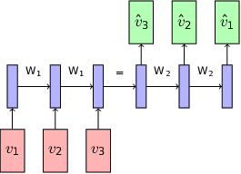

4.1 Moving MNIST for Unsupervised Sequence Learning
Goal. For pixel-level tasks, prediction quality can be understood by the uncertainty estimate, i.e., estimated model variance of that pixel. In these experiments, we ask the following questions qualitatively and quantitatively: (1) Given a visually ‘good looking’ sequence prediction, how can we tell that its trajectory is correct? (2) If it is, can we derive the degree of uncertainty on its prediction?
Experimental Setup. The moving MNIST dataset consists of MNIST digits moving within a image. A sequence of 20 frames is constructed for each training sample, where digits move randomly, bouncing when a frame edge is hit. Here, the training set consists of an infinite number of potential sequences, and at each iteration a batch of these samples is used. Following previous work on image sequences [31], we split sequences into two parts and evaluate SP-GRU in two similar but distinct network setups. First, we train an SP-GRU auto-encoder, which given the first half of a sequence, learns a hidden representation to be used in the reconstruction of that same sequence (see Fig. 5). Second, we set up a predictor SP-GRU, which learns to extrapolate the latter half of the sequence from that hidden representation. All hidden representations are of size , with parameters for each of the two natural parameters.
Controlled Moving MNIST. We first train our SP-GRU and the MC-LSTM [27] with the same number of parameters until they have similar test errors (independent of uncertainty) on simple one-digit MNIST sequences moving in a straight line (blue line in Fig. 6). We then construct three sets of ‘unfamiliar’ samples where each set consists of sequences deviating from the training sequence path with varying angle, speed and pixel-level noise.
- 1.
Angle (Fig. 6a): We show the input (first 10 triangles) and output (last 10 circles) trajectories of training angle which we train the model with. Note that this is the only path that the single digit MNIST sequences traveled. The test trajectories with the angles , and which become more ‘unfamiliar’ as it increases are tested to predict the last 10 frames (circles).
- 2.
Speed (Fig. 6b): We keep the angle (same training angle as the angle deviation setup show in Fig. 6a) and the speed ( of image size per frame) as in top left of Fig. 6b in training. Then, we increase the speed (Fig. 6b: top right, bottom left, bottom right) to , and . Thus, the trajectories all travel in the same direction but with different speeds to construct paths with unfamiliar speeds.
- 3.
Pixel-level noise: This is a simple setup where the training and testing paths all have the same angles and speeds, but pixel-level noise is added with higher intensities for testing sequences. Specifically, for each pixel a noise from Unif is added so the training has zero noise with Unif for and the testing sequences have noise with Unif for increasing .

(a) Angles


(b) Speeds
Results. For varying angle and speed deviations, (top/middle of Fig. 7), the predictions look visually sensible, but they do not actually follow the ground truth trajectories. We can quantify this directly by the sum of pixel-level variance per frame (averaged over time and testset) as shown in the right of Fig. 7. The uncertainty increases as the angle/speed deviation increases for both SP-GRU and MC-LSTM. The level of pixel-noise (bottom of Fig. 7) also increases model uncertainty (note the trajectories remain the same). These observations exactly demonstrate the usefulness of uncertainty when the prediction output itself is visually sensible.
Ground Truth
Prediction
Uncertainty


Ground Truth
Prediction
Uncertainty
%


%


%


%


Input
Prediction
Uncertainty


From a practical perspective, the uncertainty inference should not sacrifice computational speed, e.g., realtime safety of an autonomous vehicle. With respect to this crucial aspect, SP-GRU greatly benefits from its sampling-free procedure: each epoch ( sequences) takes 3 seconds while MC-LSTM with a Monte Carlo rate of requires 40 seconds ( times SP-GRU) despite their comparable qualitative performance. The MC sampling rate for these methods cannot simply be decreased: uncertainty will be underestimated. Further, theoretical analysis may be necessary to determine the rate of convergence to the true model uncertainty, if convergence is guaranteed at all. With SP-GRU, we compute this model uncertainty in closed form, without the need for any heavy lifting from large sample analysis.
Qualitative Comparisons. We demonstrated that the uncertainty measures of both SP-GRU and MC-LSTM behave similarly such that the increasing trajectory deviations had also increased the uncertainties (Fig. 7). However, the absolute magnitudes of these measures do not necessarily translate directly to the quality of uncertainty. For instance, given the same unfamiliar input, if the uncertainty of SP-GRU is higher than that of MC-LSTM, that does not necessarily mean that the uncertainty estimate of SP-GRU is better than that of MC-LSTM. Instead, the relative measure of uncertainty within each model is of more interest which demonstrates how each model appropriately detects the degree of uncertainty given various inputs.


Thus, in Fig. 8, we qualitatively show that the uncertainty measures of the models, despite the small gaps between their quantities, agree with each other. In other words, we see how the uncertainty maps from SP-GRU and MC-LSTM look similar to each other, implying that (1) these models interpret the uncertainty similarly (which is reasonable given the similarity between their basic cell structures) and (2) the between-model uncertainty gaps are of less significance.
Random Moving MNIST. We perform two learning tasks on training sequences of frames of two moving moving digits. Given the first 10 input frames, (1) reconstruct the same input frames and (2) predict the next 10 frames. We use the same test set provided by [31] to facilitate model comparison.
Results. A test sample is given in Fig. 9 (top three rows). As expected, the quality of the input reconstruction diminishes as the network progresses further into the past. We see a reflected, but similar behavior with the predictor model. Notice that these qualitative interpretations are directly quantifiable through the variance output.We briefly evaluate how well SP-GRU is able to perform on out-of-domain samples (Fig. 9, bottom three rows). Models deployed in real-world settings may not realistically be able to determine if a sample is far from their training distributions.
| Model | Test Loss |
|---|---|
| [31] Srivastava et al. | 341.2 |
| [37] Xingjian et al. | 367.1 |
| [38] Brabandere et al. | 285.2 |
| [39] Ghosh et al. | 241.8 |
| SP-GRU | 277.1 |
However, with our specific modeling of uncertainty, we would expect that images or sequences distant from the training data will exhibit high variance.


We construct sequences of 3 moving digits. In this case, future reconstruction is generally quite poor. As has been observed in previous work [31], the model attempts to hallucinate two digits. Our model is aware of this issue: the variance for a large number of pixels is extremely high, regardless of if the digits overlap. Even in “easy" cases where there is little overlap and digits are relatively clear, the model has some sense of the particular input sample and recovery being far from its learning distribution.
We compare our method to previous work in Table 2. SP-GRU with a basic predictor network setup (Fig. 2) performs comparably or better than other methods that do not provide model uncertainty. In these works, model performance often benefits from their specific network structure: encoder-predictor composite models [31], generative adversarial networks [39], and external weight filters [38]. Further, more recent models [40, 41] have achieved better results with large, more sophisticated pipelines. Extending SP-GRU to such setups becomes a reasonable modification, providing model uncertainty without sacrificing performance.
Other Methods of Measuring Uncertainty. Deep Markov Models [42] introduced recently naturally give rise to a probabilistic interpretation of predictions from deep temporal models. However, upon application of this model to Moving MNIST we were unable to obtain any reasonable prediction, across a range of hidden dimension sizes and trajectory complexities, even with significant training time (days vs. hours for SP-GRU). Shown in Fig. 10 are results using a hidden dimension size of 1024, with 100 dimensional hidden state. We note that the experimental setups described in [42] are small in dimension and complexity compared to Moving MNIST, and it may be the case that small technical development with DMMs may lead to promising and comparable uncertainty results.

5 Conclusion
Recent developments in vision and machine learning suggest that in the near term future, network-based algorithms will play an increasing role in systems deployed in healthcare, economics, scientific studies (outside of computer science) and even policy making. But to facilitate this progression, one of potentially many requirements will be the ability of the models to meaningfully reason about uncertainty. Complementary to the developing body of work on Bayesian perspectives on deep learning, this paper shows how a mix of old and new ideas can enable deriving uncertainty estimates for a powerful class of models, GRUs, which is easily extensible to other sequential models as well. While the low-level details of the approach are involved, it is intuitive and works surprisingly well in practice. We first show applications on a standard dataset used in sequential models where our results are competitive with other algorithms, while offering uncertainty as a natural byproduct. The TensorFlow implementation will be publicly available.
References
- [1] Wu, Y., Schuster, M., Chen, Z., Le, Q.V., Norouzi, M., Macherey, W., Krikun, M., Cao, Y., Gao, Q., Macherey, K., et al.: Google’s neural machine translation system: Bridging the gap between human and machine translation. arXiv preprint arXiv:1609.08144 (2016)
- [2] Jozefowicz, R., Vinyals, O., Schuster, M., Shazeer, N., Wu, Y.: Exploring the limits of language modeling. arXiv preprint arXiv:1602.02410 (2016)
- [3] Zaremba, W., Sutskever, I., Vinyals, O.: Recurrent neural network regularization. arXiv preprint arXiv:1409.2329 (2014)
- [4] Hinton, G., Vinyals, O., Dean, J.: Distilling the knowledge in a neural network. arXiv preprint arXiv:1503.02531 (2015)
- [5] Amodei, D., Ananthanarayanan, S., Anubhai, R., Bai, J., Battenberg, E., Case, C., Casper, J., Catanzaro, B., Cheng, Q., Chen, G., et al.: Deep speech 2: End-to-end speech recognition in english and mandarin. In: ICML. (2016)
- [6] Cho, K., Van Merriënboer, B., Gulcehre, C., Bahdanau, D., Bougares, F., Schwenk, H., Bengio, Y.: Learning phrase representations using RNN encoder-decoder for statistical machine translation. arXiv preprint arXiv:1406.1078 (2014)
- [7] Mikolov, T., Karafiát, M., Burget, L., Cernockỳ, J., Khudanpur, S.: Recurrent neural network based language model. In: Interspeech. Volume 2. (2010) 3
- [8] Pan, P., Xu, Z., Yang, Y., Wu, F., Zhuang, Y.: Hierarchical recurrent neural encoder for video representation with application to captioning. In: CVPR. (2016)
- [9] Yu, H., Wang, J., Huang, Z., Yang, Y., Xu, W.: Video paragraph captioning using hierarchical recurrent neural networks. In: CVPR. (2016)
- [10] Venugopalan, S., Rohrbach, M., Donahue, J., Mooney, R., Darrell, T., Saenko, K.: Sequence to sequence-video to text. In: CVPR. (2015)
- [11] Jagannatha, A.N., Yu, H.: Bidirectional rnn for medical event detection in electronic health records. In: Association for Computational Linguistics. (2016)
- [12] Esteban, C., Staeck, O., Baier, S., Yang, Y., Tresp, V.: Predicting clinical events by combining static and dynamic information using recurrent neural networks. In: ICHI. (2016)
- [13] Gers, F.A., Schmidhuber, J., Cummins, F.: Learning to forget: Continual prediction with LSTM. (1999)
- [14] Chung, J., Gulcehre, C., Cho, K., Bengio, Y.: Empirical evaluation of gated recurrent neural networks on sequence modeling. arXiv preprint arXiv:1412.3555 (2014)
- [15] Fortunato, M., Blundell, C., Vinyals, O.: Bayesian Recurrent Neural Networks. arXiv preprint arXiv:1704.02798 (2017)
- [16] Lambert, J., Greer, P.B., Menk, F., Patterson, J., Parker, J., Dahl, K., Gupta, S., Capp, A., Wratten, C., Tang, C., et al.: MRI-guided prostate radiation therapy planning: Investigation of dosimetric accuracy of MRI-based dose planning. Radiotherapy and Oncology 98(3) (2011) 330–334
- [17] Der Kiureghian, A., Ditlevsen, O.: Aleatory or epistemic? does it matter? Structural Safety 31(2) (2009) 105–112
- [18] Kendall, A., Gal, Y.: What Uncertainties Do We Need in Bayesian Deep learning for Computer Vision? In: NIPS. (2017)
- [19] MacKay, D.J.: Bayesian methods for adaptive models. PhD thesis, California Institute of Technology (1992)
- [20] Hinton, G.E., Van Camp, D.: Keeping the neural networks simple by minimizing the description length of the weights. In: Computational learning theory. (1993)
- [21] MacKay, D.J.: A practical Bayesian framework for backpropagation networks. Neural computation 4(3) (1992) 448–472
- [22] Graves, A.: Practical variational inference for neural networks. In: NIPS. (2011)
- [23] Hernández-Lobato, J.M., Adams, R.: Probabilistic backpropagation for scalable learning of bayesian neural networks. In: ICML. (2015)
- [24] Blundell, C., Cornebise, J., Kavukcuoglu, K., Wierstra, D.: Weight uncertainty in neural networks. arXiv preprint arXiv:1505.05424 (2015)
- [25] Welling, M., Teh, Y.W.: Bayesian learning via stochastic gradient Langevin dynamics. In: ICML. (2011)
- [26] Rasmussen, C.E., Quinonero-Candela, J.: Healing the relevance vector machine through augmentation. In: ICML. (2005)
- [27] Gal, Y., Ghahramani, Z.: Dropout as a Bayesian approximation: Representing model uncertainty in deep learning. In: ICML. (2016)
- [28] Srivastava, N., Hinton, G.E., Krizhevsky, A., Sutskever, I., Salakhutdinov, R.: Dropout: a simple way to prevent neural networks from overfitting. JMLR 15(1) (2014) 1929–1958
- [29] Lakshminarayanan, B., Pritzel, A., Blundell, C.: Simple and Scalable Predictive Uncertainty Estimation using Deep Ensembles. arXiv preprint arXiv:1612.01474 (2016)
- [30] Wang, H., Xingjian, S., Yeung, D.Y.: Natural-parameter networks: A class of probabilistic neural networks. In: NIPS. (2016)
- [31] Srivastava, N., Mansimov, E., Salakhudinov, R.: Unsupervised learning of video representations using lstms. In: ICML. (2015)
- [32] Jozefowicz, R., Zaremba, W., Sutskever, I.: An empirical exploration of recurrent network architectures. In: International Conference on Machine Learning. (2015) 2342–2350
- [33] Ranganath, R., Tang, L., Charlin, L., Blei, D.: Deep exponential families. In: Artificial Intelligence and Statistics. (2015) 762–771
- [34] Greff, K., Srivastava, R.K., Koutník, J., Steunebrink, B.R., Schmidhuber, J.: LSTM: A search space odyssey. NNLS (2017)
- [35] Athiwaratkun, B., Stokes, J.W.: Malware classification with LSTM and GRU language models and a character-level CNN. In: ICASSP. (2017)
- [36] Kingma, D., Ba, J.: Adam: A method for stochastic optimization. arXiv preprint arXiv:1412.6980 (2014)
- [37] Xingjian, S., Chen, Z., Wang, H., Yeung, D.Y., Wong, W.K., Woo, W.c.: Convolutional lstm network: A machine learning approach for precipitation nowcasting. In: NIPS. (2015)
- [38] De Brabandere, B., Jia, X., Tuytelaars, T., Van Gool, L.: Dynamic filter networks. In: NIPS. (2016)
- [39] Ghosh, A., Kulharia, V., Mukerjee, A., Namboodiri, V., Bansal, M.: Contextual rnn-gans for abstract reasoning diagram generation. arXiv preprint arXiv:1609.09444 (2016)
- [40] Cricri, F., Honkala, M., Ni, X., Aksu, E., Gabbouj, M.: Video ladder networks. arXiv preprint arXiv:1612.01756 (2016)
- [41] Kalchbrenner, N., Oord, A.v.d., Simonyan, K., Danihelka, I., Vinyals, O., Graves, A., Kavukcuoglu, K.: Video pixel networks. arXiv preprint arXiv:1610.00527 (2016)
- [42] Krishnan, R.G., Shalit, U., Sontag, D.: Structured inference networks for nonlinear state space models. In: AAAI. (2017) 2101–2109
Appendix A Nonlinear Transformations of Other Exponential Family Distributions
We show the activation functions (nonlinear transformations) of some common exponential family distributions. As we mentioned in the main text, the closed form solutions of the nonlinear transformations (Sec. 3.3) of several exponential family distributions involves a monotonically increasing and bounded ’activation-like’ mapping where is an arbitrary activation of choice with appropriate constants , and . Using , the goal is to perform nonlinear transformations on the pre-activation output with respect to mean and variance , equivalent to the following marginals:
| (9) |
which we express in closed forms. We refer to [30] to show the derivations for Gamma, Poisson and Gaussian distributions.
A.1 Gamma Distribution
The probability density function (pdf) of the Gamma distribution given parameters and (not to be confused with natural parameters as these are conventional notations) is
for the support and . Then, let , and to get . We first perform a nonlinear transformation with respect to as follows:
and for the variance,
for and where and are generally good choices that resemble .
A.2 Poisson Distribution
The pdf of the Poisson distribution over the support with a parameter is
| (10) |
Then, let , and to get . The nonlinear transformation on to obtain is as follows:
and for the variance,
for and .
A.3 Gaussian Distribution
Here, we provide details of the nonlinear transformation on the Gaussian distribution (Eq. (5,6,7,8) of main text). Note that our goal is to compute
for some nonlinear function , mean and variance . First, we consider . Then, Eq. A.3 is the logistic-normal integral:
which does not have a closed form solution. Now, we use the fact that a probit function
can be used to approximate a sigmoid function such that
for . Further, we know that
so the nonlinear transformation on with respect to is
for . Similarly, for the variance, since
for and , we see that
for .
The hyperbolic tangent function can be derived in a similar way since . Thus, for over the support ,
and for the variance,
where and .