Imprints of Oscillatory Bispectra on Galaxy Clustering

The scale dependence of the bias of tracers of the dark matter density field (e.g. dark matter halos) is a prominent signature of primordial non-Gaussianity on large-scale structure [6, 7, 8, 9]. For Gaussian initial conditions, the number density of halos on scales larger than the halo Lagrangian radius $R_{\ast}$, i.e. in a region of size $R_{L}\gg R_{\ast}$, depends on the average of the matter density in that region (and its gradients). There is also dependence on the amplitude of matter fluctuations on scales smaller than $R_{L}^{-1}$: however, in absence of a coupling between long- and short-wavelength modes in the initial conditions, this dependence only affects the tracer statistics on large scales by adding a white-noise term to the otherwise deterministic relation between their number density and the matter density. Things change for non-Gaussian initial conditions. In this case there are large-scale modulations of the small-scale fluctuations, due to mode coupling. This leads, in general, to a dependence on both the amplitude and the shape of the small-scale matter power spectrum: both are correlated with long-wavelength perturbations, in a way that is encoded by the squeezed-limit bispectrum. Famously, for local primordial non-Gaussianity, where the primordial bispectrum takes the form $B_{\phi}(\bm{k}_{1},\bm{k}_{2},\bm{k}_{3})=2f_{\mathrm{NL}}^{\mathrm{loc}}\big(P_{\phi}(k_{1})P_{\phi}(k_{2})+\text{2 perms.}\big)$, the amplitude of small-scale fluctuations is uniformly rescaled by the gravitational potential, leading to a scale-dependent bias that increases as $k^{-2}$ on large scales relative to matter [10]. Looking for this scale dependence in galaxy surveys can place constraints on non-Gaussianity that are competitive with those from the CMB: future large-volume galaxy surveys can in principle reach the precision of $\sigma(f_{\mathrm{NL}}^{\mathrm{loc}})\lesssim$1$$ [11, 12, 13, 14, 15, 16], and can go down to $\sigma(f_{\mathrm{NL}}^{\mathrm{loc}})\approx$0.2$$ when measurements of the galaxy bispectrum are included [17].

While sizable local non-Gaussianity is generically expected in multi-field inflationary models, things are different in single-clock inflation. Here, the leading behavior of the bispectrum in the squeezed limit is determined by the so-called consistency relation [18, 19], which relates it to the tilt of the power spectrum, giving $f_{\mathrm{NL}}^{\text{loc}}=1-n_{\text{s}}$. However, such consistency relation cancels from any local observable [20, 21, 22, 23]: when discussing dark matter tracers this is just the statement that, with adiabatic initial conditions, their clustering is not sensitive to the local scale factor, but can be affected only by the local curvature and the local Hubble rate [24, 25, 26, 9]. This “separate universe” picture is made explicit by working in Conformal Fermi Coordinates (CFC) [21, 22]: in CFC the squeezed bispectrum contains only the physical part of the couplings between long and short modes set up by inflation, which can actually affect the dynamics once the modes re-enter the Hubble radius.

Consider, then, the squeezed-limit expansion in powers of $k_{\ell}/k_{s}$, where $k_{\ell}^{-1}$ and $k_{s}^{-1}$ are, respectively, the scale at which we measure correlations and the size of the tracers we are looking at. If the consistency relation holds, using CFC one can show that the first physical effect from the initial conditions arises at order $(k_{\ell}/k_{s})^{2}$ [20]. For some particular inflationary models, however, this conclusion is too quick. Consider for example the case of an inflaton speed of sound $c^{2}_{\mathrm{s}}\ll 1$: in this case, there is an enhancement $\sim c^{-2}_{\mathrm{s}}(k_{\ell}/k_{s})^{2}$ in the squeezed limit [27]. Another example is that of axion monodromy-inspired models of inflation [28, 29, 30], where the slow-roll potential possesses small sinusoidal modulations. In these models, the bispectrum has a specific shape (called resonant non-Gaussianity) which has little overlap with all other bispectrum templates [31]. The bispectrum satisfies the consistency relation [31], but deviations appear at order $\alpha k_{\ell}/k_{s}$, where $\alpha\gg 1$ is the frequency of the oscillations of the background in units of the Hubble rate [32, 33, 20]. This is due to the fact that in the regime of rapid oscillations, the modifications in the power spectrum come from resonant production of inflaton quanta of comoving momentum $k$ happening at $\frac{k}{aH}\sim\alpha$, i.e. when the mode is a factor $\alpha$ shorter than the Hubble radius. For the long mode to act as a modification of the background for the short modes, it had to be well outside the Hubble radius not only at the time of Hubble exit of the short modes, but already when they were in resonance [31, 32]. A third example is Khronon inflation [34]: in this case the time dependence of the curvature perturbation $\zeta(k)$ does not start at order $k^{2}$ as in the standard scenario, so there is a non-trivial contribution at order $k_{\ell}$ in the squeezed limit, which corresponds to a non-local term $\propto\sqrt{\partial^{2}}\zeta$. However, this contribution will be suppressed by the deviation from scale invariance, i.e. by slow-roll, so the final result is too small to be of interest.

A second family of models that show a peculiar behavior in the squeezed limit are the so-called “cosmological collider” models. Here, the inflaton is coupled to other massive fields that can have non-zero spin: the conversion of a long-wavelength massive particle into curvature perturbations can generate long-short mode couplings and leave an imprint on the squeezed bispectrum [35, 36, 37, 38]. While the consistency relation is satisfied, i.e. the term $\propto(k_{\ell}/k_{s})^{0}$ is fixed by $1-n_{\mathrm{s}}$, it is possible to have a non-analytical dependence of the scalar bispectrum on $k_{\ell}/k_{s}$ at sub-leading order in the squeezed limit: indeed, while some of the effects of the interaction can be mimicked by adding local vertices to the Lagrangian of the Goldstone boson $\pi$ of broken time diffeomorphisms (as a result of integrating out these massive fields), spontaneous particle production in an expanding spacetime will lead to effects that are inherently non-local. As an example, consider a massive scalar field $\sigma$ coupled to $\pi$: if $m\geq 3H/2$ the bispectrum will show an oscillatory behavior with $k_{\ell}/k_{s}$, while fields with $0<m<3H/2$ will lead to scalings $(k_{\ell}/k_{s})^{3/2-\nu}$, where $\nu=\sqrt{9/4-m^{2}/H^{2}}$. While these non-analytical scalings are suppressed by $\exp({-{\pi m}/{H}})$, it is possible to obtain some observable effect in the limit of small sound speed for $\pi$ [38]. Unlike isocurvature modes, the energy density due to massive particles becomes quickly diluted during inflation, so that they do not have any effects on observables after the end of inflation. In other words, the relationship between the adiabatic mode $\pi$ at the end of inflation and the conserved quantity $\zeta$ is the same as in the single-clock case. This allows us, again, to study the effect of this primordial non-Gaussianity on the scale-dependent bias by working in Conformal Fermi Coordinates, i.e. by computing the squeezed CFC bispectrum.

One last class of single-field models known as Ultra Slow-Roll inflation [39] is well-known for its peculiar features in the squeezed-limit bispectrum [40, 41, 42]. New soft theorems in this class of models have been recently discussed in [43, 44, 45, 46], together with their implications for late-universe observables [47]. Here, we will not discuss them further.

The goal of this paper is to compute the scale-dependent bias in these inflationary models. Among the single-clock models discussed above, we are going to focus only on the case of resonant non-Gaussianity: this was originally investigated in [48] (which, however, included the unphysical contribution from the consistency relation). For the cosmological collider models, we consider only the case of a spin-$0$ field with $m\geq 3H/2$ (the more general case was recently investigated in [49]).

The paper is organized as follows: in Section 2 we review the concept of bias in General Relativity following [24], matching to the results of [22]: the technical details of how to use the calculation of CFC bispectrum during inflation as the initial condition for the late-time evolution are collected in Appendix A. In Section 3 we compute the CFC bispectrum for resonant non-Gaussianity, and discuss the results for the bias in Section 4 (some theoretical details on the calculation of the bias are collected in Appendix B, while two additional plots are shown in Appendix C). Section 5 does the same for cosmological collider models. We conclude in Section 6. Appendix D contains the details of the calculation of the CFC bispectrum in cosmological collider models.

Then, halos will form as if they were living in a different background FLRW, and we can define bias as how a family of inertial observers living in the patch sees the number density of halos depend on the mean curvature that they measure in the patch.¹¹ 1 This must then be connected to what is actually measured by an observer on Earth. However, these “projection effects” are independent of the dynamics, and can be computed separately, for example with the so-called ruler perturbations of [51, 52, 53] (see also [54, 55, 56] for similar approaches). In Conformal Fermi Coordinates $(t_{F},\bm{x}_{F}=\bm{q})$, where $t_{F}$ is the proper time and $\bm{q}$ is the Lagrangian coordinate of comoving observers with the matter fluid, this “separate universe picture” is manifest, and we can define the Eulerian bias as

$$b_{K_{F}}^{E}\equiv-\frac{\partial\log\braket{n_{h}^{E}(t_{F},\bm{q})}}{\partial\Omega_{K_{F}}}\bigg|_{K_{F}=0}\,\,,\qquad\Omega_{K_{F}}=-\frac{K_{F}}{a^{2}_{F}H^{2}_{F}}\,\,,$$

(1)

i.e. as the derivative of the proper density of halos of a given mass, averaged in the CFC patch, with respect to the contribution of the local curvature to the energy density. The definition that is usually used in the literature is different from Eq. (1): indeed one defines the bias $b_{1}^{E}$ as a derivative with respect to the local density using the relation between $K_{F}$ and the synchronous-gauge density perturbation, i.e.

$$K_{F}=\frac{5}{3}\frac{\Omega_{\mathrm{m}}H^{2}_{0}}{D_{1}(\eta)}\delta_{\text{sc}}(\eta)\,\,,$$

(2)

where $D_{1}(\eta)$ is the linear growth factor normalized to $a(\eta)$ during matter domination. In the rest of this paper we are going to use the Lagrangian bias $b_{1}$ as bias parameter, i.e.²² 2 The relation between the Lagrangian and Eulerian biases is determined by $$1+\delta_{h}^{E}=(1+\delta_{h})(1+\delta_{\text{sc}})=1+(1+b_{1})\delta_{\text{sc}}\,\,,$$ where $\delta_{h}$ and $\delta_{h}^{E}$ are the fractional Lagrangian and Eulerian halo density perturbations at fixed proper time, respectively.

$$b_{1}=b_{1}^{E}-1=\frac{5}{3}\frac{\Omega_{\mathrm{m}}H^{2}_{0}}{D_{1}(\eta)}\frac{b_{K_{F}}}{a^{2}_{F}H^{2}_{F}}-1\,\,.$$

(3)

Non-linear gravitational evolution will contribute to the coupling of the short-scale modes to local curvature (mainly through the modification to the expansion history if the speed of sound is small), thereby contributing to the derivative in Eq. (1) and then to $b_{1}$. Therefore, if the initial small-scale perturbations are not correlated with the long-wavelength mode, $b_{1}$ captures the full dependence of the halo number density on it (at leading order in derivatives and in perturbations). However, some contribution will also come from the initial conditions, i.e. by the long-short mode coupling during inflation. Here CFC are again very useful. Indeed, we can use them to follow both short and long modes from when they leave the Hubble radius during inflation to Hubble re-entry during radiation or matter dominance (this would not have been possible had we used standard Fermi Normal Coordinates, since they can be trusted only far inside the Hubble scale): more precisely, it is enough to work at linear order in perturbation theory for the short modes in the curved separate universe described by CFC. The initial conditions for the Newtonian potentials, then, are simply given by

$$\phi_{s}^{F}=\psi_{s}^{F}=-\frac{3(1+w)}{5+3w}\zeta_{s}^{F}\,\,,$$

(4)

where we have defined the potentials $\phi_{s}^{F}$ and $\psi_{s}^{F}$ in Newtonian gauge by

$$\mathrm{d}s^{2}=a^{2}_{F}\bigg[{-(1+2\phi^{F}_{s})\mathrm{d}\eta^{2}_{F}}+\frac{(1-2\psi^{F}_{s})\mathrm{d}\bm{x}_{F}^{2}}{(1+K_{F}\lvert\bm{x}_{F}\rvert^{2}/4)^{2}}\bigg]\,\,.$$

(5)

The procedure is delineated in Appendix A: it amounts to computing the relation between the gauge-invariant curvature perturbation on constant energy hypersurfaces in a curved FLRW background and the short-scale metric perturbations in Newtonian gauge. We can already understand why Eq. (4) will hold by recalling that the corrections coming from curvature will scale as $\Omega_{K_{F}}/H^{2}_{F}=-K_{F}/(a^{2}_{F}H^{2}_{F})$, which is exponentially diluted during inflation. All that is left, then, is how interactions during inflation couple $\zeta_{s}^{F}$ to $K_{F}$. These are the initial conditions that one can use, e.g., in a separate universe simulation: for example, one can run numerical codes such as CAMB [57] with non-zero curvature and modified expansion history and an initial power spectrum for the comoving curvature perturbation equal to the one in CFC [24, 25, 26].³³ 3 Of course, to be able to treat $K_{F}$ as a constant throughout, the long mode must re-enter the Hubble radius during matter dominance.

What about the coupling with $K_{F}$ or, equivalently, the squeezed bispectrum of the comoving curvature perturbation in CFC? This can be derived in a number of ways [27, 50], but the most straightforward way is to realize that, if we are in presence of an isotropic long mode $\zeta_{\ell}$, the long-wavelength part of the metric during inflation is already of the same form of that of a curved FLRW, apart from corrections that decay as the universe expands. Indeed, let us consider comoving gauge and neglect tensor modes: at linear order in perturbations, the metric takes the form

$$\begin{split}&\mathrm{d}s^{2}=a^{2}(\eta)\big[{-\big(1+2{\delta N_{\ell}}(\eta,\bm{x})\big)\mathrm{d}\eta^{2}}\\ &\hphantom{\mathrm{d}s^{2}=a^{2}(\eta)\big[}+N_{i,\ell}(\eta,\bm{x})(\mathrm{d}\eta\mathrm{d}x^{i}+\mathrm{d}x^{i}\mathrm{d}\eta)\\ &\hphantom{\mathrm{d}s^{2}=a^{2}(\eta)\big[}+\big(1+2\zeta_{\ell}(\eta,\bm{x})\big)\mathrm{d}\bm{x}^{2}\big]+\mathcal{O}(\zeta_{\ell}^{2})\,\,.\end{split}$$

(6)

At this order, using the isotropy of the long mode (i.e. $\partial_{i}\zeta_{\ell}(\eta,\bm{0})=0$ and $\partial_{i}\partial_{j}\zeta_{\ell}(\eta,\bm{0})=\partial^{2}\zeta_{\ell}(\eta,\bm{0})\delta_{ij}/3$), we can rewrite the spatial part as

$$g_{ij}=\frac{a^{2}(\eta)\big[1+2\zeta_{\ell}(\eta,\bm{0})\big]\delta_{ij}}{\Big(1+\frac{K_{F}\lvert\bm{x}\rvert^{2}}{4}\Big)^{2}}+\mathcal{O}(\bm{x}^{3},\zeta_{\ell}^{2})\,\,,$$

(7)

where $K_{F}=-2\partial^{2}\zeta_{\ell}(\eta,\bm{0})/3$. The solutions for the lapse and shift constraints, i.e. [18]

		$\displaystyle\delta N_{\ell}=\frac{\zeta^{\prime}_{\ell}}{\mathcal{H}}\,\,,$		(8a)
		$\displaystyle N_{i,\ell}=\partial_{i}\bigg({-\frac{\zeta_{\ell}}{\mathcal{H}}}+\varepsilon\partial^{-2}\zeta^{\prime}_{\ell}\bigg)\,\,,$		(8b)

decay at late times (indeed, since we assume that the vacuum is the Bunch-Davies one and that the background has already reached the attractor, the time dependence of $\zeta$ starts at order $k^{2}$: $\zeta^{\prime}\sim k^{2}\eta$). Notice that here by “late times” we mean the transition from the inflationary phase to the Hot Big Bang phase. To find the initial conditions on super-Hubble scales for the evolution of perturbations in the epoch of radiation or matter dominance one takes the $\eta\to 0$ limit during the inflationary phase, when the expansion is close to de Sitter, $\mathcal{H}=-1/\eta$ (see [18] and [58] for a calculation up to second order in perturbations). To summarize, this tells us that the CFC scale factor will asymptote to its unperturbed value at late times [27, 50], and only the correction to the local curvature $K_{F}$, which is conserved on super-horizon scales, will survive.⁴⁴ 4 As shown in [50], there are $\mathcal{O}(\varepsilon)$ tidal fields, that in any case vanish for an isotropic long mode.

Therefore, in the case of an isotropic long mode, the CFC calculation simplifies greatly, and reduces to that of [20]: more precisely, up to and including $\mathcal{O}(k^{2}_{\ell}/k^{2}_{s})$, the super-Hubble squeezed CFC bispectrum takes the form

$$\begin{split}B_{\zeta}^{F}(k_{\ell},k_{s})&=B_{\zeta}(k_{\ell},k_{s})-\frac{\mathrm{d}\log\big(k_{s}^{3}P_{\zeta}(k_{s})\big)}{\mathrm{d}\log k_{s}}P_{\zeta}(k_{\ell})P_{\zeta}(k_{s})\\ &\equiv B_{\zeta}(k_{\ell},k_{s})-\Delta B_{\zeta}(k_{\ell},k_{s})\,\,,\end{split}$$

(9)

where $B_{\zeta}(k_{\ell},k_{s})$ is the squeezed bispectrum in global coordinates, averaged over the angle $\cos\theta$ between $\bm{k}_{\ell}$ and $\bm{k}_{s}$:

$$\int_{-1}^{1}\frac{\mathrm{d}\cos\theta}{2}\lim_{\bm{k}_{\ell}\rightarrow 0}\braket{\zeta(\bm{k}_{1})\zeta(\bm{k}_{2})\zeta(\bm{k}_{\ell})}\equiv(2\pi)^{3}\delta^{(3)}(\bm{k}_{1}+\bm{k}_{2}+\bm{k}_{\ell})B_{\zeta}(k_{\ell},k_{s})\,\,,$$

(10)

with $\bm{k}_{1}=\bm{k}_{s}-\bm{k}/2$, $\bm{k}_{2}={-\bm{k}_{s}}-\bm{k}/2$. Since the bias is sensitive only to the angle-average of the squeezed-limit bispectrum, Eq. (9) is all we need to compute the contribution to $b_{1}$ from the initial conditions. We start by considering the case of resonant non-Gaussianity.

As discussed in [32, 20, 50], the squeezed bispectrum $B_{\zeta}$ should not contain terms proportional to $k_{\ell}/k_{s}$, if $\bm{k}_{s}$ and $\bm{k}_{\ell}$ are defined as

$$\bm{k}_{1}=\bm{k}_{s}-\frac{\bm{k}_{\ell}}{2}\,\,,\qquad\bm{k}_{2}={-\bm{k}_{s}}-\frac{\bm{k}_{\ell}}{2}\,\,,\qquad\bm{k}_{3}=\bm{k}_{\ell}\,\,.$$

(15)

Instead, such linear terms do appear when expanding the three leading order terms in Eq. (12). The reason for their presence is the following. The bispectrum in global coordinates is computed as an expansion in $\alpha^{-1}$, and at a fixed order $\alpha^{-n}$, the term proportional to $\alpha^{-n}\times(k_{\ell}/k_{s})$ in the squeezed limit will be cancelled by⁵⁵ 5 This is seen explicitly in Eq. (12): since the explicit terms go up to order $\alpha^{-2}$, there are no terms $\sim\alpha^{-1}\times(k_{\ell}/k_{s})$ in the squeezed global bispectrum (and then in the CFC transformation). a contribution coming from the term of order $\alpha^{-(n+1)}$ [32]. So, if we do not include $B_{\zeta}^{\text{ho}}$ we do not find a cancellation at order $\alpha^{-2}$. To fix this problem, we keep a contribution from the higher order term that in the squeezed limit takes precisely the right form to cancel all $k_{\ell}/k_{s}$ terms at order $\alpha^{-2}$:

$$B_{\zeta}^{\text{ho}}(k_{\ell},k_{s})\supset{-f_{\mathrm{NL}}^{\mathrm{res}}}\frac{8}{\alpha^{2}}\frac{k_{\ell}}{k_{s}}\sin\bigg(\alpha\log\frac{2k_{s}}{k_{\ast}}\bigg)P_{\zeta}(k_{\ell})P_{\zeta}(k_{s})\,\,.$$

(16)

By including this term but neglecting the corresponding term of order $\alpha^{-3}$ in the bispectrum in global coordinates of Eq. (12), we are making an error of order $\alpha^{-3}$, which is negligible for any foreseeable application (as we will see in Section 4.1). The CFC correction $\Delta B_{\zeta}$ is simply computed from the power spectrum of Eq. (13):

$$\Delta B_{\zeta}(k_{\ell},k_{s})\equiv f_{\mathrm{NL}}^{\mathrm{res}}\bigg\{\frac{8}{\alpha}\bigg[\cos\bigg(\alpha\log\frac{2k_{s}}{k_{\ast}}\bigg)-\frac{2}{\alpha}\sin\bigg(\alpha\log\frac{2k_{s}}{k_{\ast}}\bigg)\bigg]\bigg\}P_{\zeta}(k_{\ell})P_{\zeta}(k_{s})\,\,.$$

(17)

In summary, the CFC squeezed bispectrum is given by

$$\boxed{\begin{split}B^{F}_{\zeta}&=B_{\zeta}+B^{\text{ho}}_{\zeta}-\Delta B_{\zeta}\\ &=f_{\mathrm{NL}}^{\mathrm{res}}\bigg[2\alpha\cos\bigg(\alpha\log\frac{2k_{s}}{k_{\ast}}\bigg)-\frac{10}{3}\sin\bigg(\alpha\log\frac{2k_{s}}{k_{\ast}}\bigg)+\dots\bigg]\frac{k^{2}_{\ell}}{k^{2}_{s}}P_{\zeta}(k_{\ell})P_{\zeta}(k_{s})+\mathcal{O}\bigg(\frac{k^{3}_{\ell}}{k^{3}_{s}}\bigg)\,\,.\end{split}}$$

(18)

Some comments are in order:

• •

  subleading corrections in $\alpha^{-1}$ to the bispectrum of Eq. (12) will correct Eq. (18) only at order $\alpha^{-3}\times(k_{\ell}^{2}/k_{s}^{2})$;

• •

  at a fixed value of $k_{\ell}/k_{s}$, we see that the “physical” term of order $k_{\ell}^{2}/k_{s}^{2}$ is enhanced for large $\alpha$;

• •

  at order $(k_{\ell}/k_{s})^{0}$, the term out of phase with the tilt of the power spectrum is cancelled by the contribution of order $\alpha^{-3}$ to Eq. (12).

Having derived the CFC bispectrum, in the next section we briefly discuss what is the maximum value of $f_{\mathrm{NL}}^{\mathrm{res}}$ currently allowed by data. Then, in Section 4 we discuss how the correction to $b_{1}$ from general primordial non-Gaussianity can be computed in practice, and show the results for the resonant case.

Let us expand the bispectrum of the Newtonian potential $\phi$ in this limit. Following [9], we can write (using Eq. (15) as the definition of $\bm{k}_{i}$ in terms of $\bm{k}_{s}$, $\bm{k}_{\ell}$)

$$\begin{split}&B_{\phi}(\bm{k}_{1},\bm{k}_{2},\bm{k}_{\ell})=A(\bm{k}_{s},\bm{k}_{\ell})P_{\phi}(k_{s})P_{\phi}(k_{\ell})+\mathcal{O}(k^{2}_{\ell}/k^{2}_{s})\\ &\hphantom{B_{\phi}(\bm{k}_{1},\bm{k}_{2},\bm{k}_{\ell})}=\sum_{J=0,2,\dots}A_{J}(k_{s},k_{\ell})\mathcal{L}_{J}(\cos\theta)P_{\phi}(k_{s})P_{\phi}(k_{\ell})+\mathcal{O}(k^{2}_{\ell}/k^{2}_{s})\,\,,\end{split}$$

(19)

where $\mathcal{L}_{J}$ are the Legendre polynomials and we have defined $\cos\theta=\hat{\bm{k}}_{s}\cdot\hat{\bm{k}}_{\ell}$. Notice that only even Legendre polynomials can appear in the squeezed-limit expansion: indeed, we can interpret the squeezed bispectrum as a modulation by a long-wavelength mode $\phi(\bm{k}_{\ell})$ of the local power spectrum $P_{\phi}(\bm{k}_{s}|\bm{q})$ in a patch much smaller than the wavelength of this mode (that we center in $\bm{q}=0$ for simplicity). Since this is the power spectrum of a real field, we must have $P_{\phi}(\bm{k}_{s}|\bm{q})=P_{\phi}({-\bm{k}_{s}}|\bm{q})$.

Let us now assume for a moment that $A_{J}(k_{s},k_{\ell})=4a_{J}(k_{\ell}/k_{s})^{\Delta}$ (the factor of $4$ is conventional), and focus on the $J=0$ case (since we are interested in the bias, which is sensitive only to the monopole of the bispectrum). Eq. (19) tells us that the local power spectrum of the short-scale perturbations in this patch is modulated as

$$P_{\phi}(\bm{k}_{s}|\bm{q})=\bigg[1+4a_{0}\phi(\bm{k}_{\ell})\bigg(\frac{k_{\ell}}{k_{s}}\bigg)^{\Delta}e^{i\bm{k}_{\ell}\cdot\bm{q}}\bigg]P_{\phi}(k_{s})\,\,.$$

(20)

For $\Delta=0$, we see that the amplitude of the small-scale power spectrum is uniformly enhanced by the long mode, while for $\Delta\neq 0$ we see that also its shape is affected. Since the modulation of $P_{\phi}(k_{s})$ is mediated by $\Psi^{(\Delta)}(\bm{k}_{\ell})\equiv k_{\ell}^{\Delta}\phi(\bm{k}_{\ell})$, we see that at leading order in the squeezed limit we need to include in the bias expansion the following operator, written in terms of the Lagrangian coordinate $\bm{q}$:

$$\Psi^{(\Delta)}(\bm{q})=\int\frac{\mathrm{d}^{3}k}{(2\pi)^{3}}k^{\Delta}\phi(\bm{k})e^{i\bm{k}\cdot\bm{q}}\,\,.$$

(21)

If we want to go beyond the squeezed limit, we need to take the expansion of Eq. (19) to higher order, i.e. (focusing on the $J=0$ case)

$$\begin{split}&A_{0}(k_{s},k_{\ell})=4\sum_{n=0}^{+\infty}a_{0,2n}\bigg(\frac{k_{\ell}}{k_{s}}\bigg)^{\Delta+2n}\,\,,\end{split}$$

(22)

where we let the sum run over even powers of $k_{\ell}/k_{s}$, since odd powers would correspond to non-local couplings like, e.g., $\delta_{h}\sim\sqrt{\partial^{2}}\zeta$ for $\Delta=0$ and $n=1/2$. From this we see that we need to add the operators $\Psi^{(\Delta+2)},\Psi^{(\Delta+4)},\dots$ to the bias expansion, with the corresponding bias coefficients $b_{\Psi^{(\Delta+2n)}}$. Moreover, spatial derivatives of these operators will be present as well, i.e. we need to include operators like $\sim\partial^{2+2m}\Psi^{(\Delta+2n)}$.

Let us now go back to the squeezed limit $n=0$. Eq. (20) suggests a way to derive the actual values of the bias coefficient $b_{\Psi^{(\Delta)}}$: we need to include the modulation of the short modes induced by the squeezed bispectrum in the initial small-scale density fluctuations, follow the halo formation, and then compute the response of the halo number density to variations in $a_{0,0}\Psi^{(\Delta)}$. As we see from Eq. (20), for some infinitesimal $a_{0,0}\Psi^{(\Delta)}=\epsilon$ the rescaling of the initial $\delta_{\text{m}}(\bm{k})$ takes the form

$$\delta_{\text{m}}(\bm{k})\to\big[1+2\epsilon k^{-\Delta}\big]\delta_{\text{m}}(\bm{k})\,\,.$$

(23)

Then, calling $\macc@depth\char 1\relax\macc@set@skewchar\macc@nested@a 111{n}_{h}$ the average density of halos inside the patch over which the long mode is slowly-varying (from now on we will follow the notation of [9]), the bias coefficient $b_{\Psi^{(\Delta)}}$ is given by

$$b_{\Psi^{(\Delta)}}=\frac{\partial\log\macc@depth\char 1\relax\macc@set@skewchar\macc@nested@a 111{n}_{h}}{\partial\epsilon}\bigg|_{\epsilon=0}\,\,.$$

(24)

In the case of local-type non-Gaussianity $(\Delta=0)$, this was explicitly verified using simulations by [26, 66]. One can also straightforwardly extend this to higher orders in the squeezed limit, i.e. compute $b_{\Psi^{(\Delta+2n)}}$, by sending $\Delta\to\Delta+2n$ in Eq. (23). Let us now assume that in the Gaussian case the number density of halos depends on the small-scale power spectrum through its variance on some scale $R$, that we take to be the Lagrangian radius $R_{\ast}=R_{\ast}(M)$ (where $M$ is the halo mass). Then, by dimensional analysis, we can expect that $b_{\Psi^{(\Delta+2n)}}\sim R_{\ast}^{\Delta+2n}$. This can be seen explicitly if we consider the case of a universal mass function, i.e.

$$\macc@depth\char 1\relax\macc@set@skewchar\macc@nested@a 111{n}_{h}=\macc@depth\char 1\relax\macc@set@skewchar\macc@nested@a 111{n}_{h}(\macc@depth\char 1\relax\macc@set@skewchar\macc@nested@a 111{}_{\text{m}},\sigma_{\ast})\bigg\lvert\frac{\mathrm{d}\log\sigma_{\ast}}{\mathrm{d}\log M}\bigg\rvert\,\,,$$

(25)

where $\macc@depth\char 1\relax\macc@set@skewchar\macc@nested@a 111{}_{\text{m}}$ is the average matter density in the patch, and the variance over $R_{\ast}$ is defined as

$$\sigma^{2}_{\ast}=\int\frac{\mathrm{d}^{3}k}{(2\pi)^{3}}W^{2}_{\ast}(k)P_{\text{m}}(k)\,\,,$$

(26)

with $W_{\ast}(k)=3j_{1}(kR_{\ast})/(kR_{\ast})$ being the Fourier transform of a spherical top-hat filter with radius $R_{\ast}$. Indeed, fixing for a moment $n=0$, we can use the fact that under the transformation of Eq. (23) the variance and the Jacobian $J=\lvert\mathrm{d}\log\sigma_{\ast}/\mathrm{d}\log M\rvert$ transform as

		$\displaystyle\sigma^{2}_{\ast}\to\bigg[1+2\epsilon\frac{\sigma^{2}_{\ast,-\Delta/2}}{\sigma^{2}_{\ast}}\bigg]\sigma^{2}_{\ast}\,\,,$		(27a)
		$\displaystyle J\to\bigg[1+4\epsilon\frac{\sigma^{2}_{\ast,-\Delta/2}}{\sigma^{2}_{\ast}}\bigg(\frac{\mathrm{d}\log\sigma^{2}_{\ast,-\Delta/2}}{\mathrm{d}\log\sigma^{2}_{\ast}}-1\bigg)\bigg]J\,\,,$		(27b)

where the generalized spectral moment $\sigma^{2}_{\ast,p}$ is defined as

$$\sigma^{2}_{\ast,p}\equiv\int\frac{\mathrm{d}^{3}k}{(2\pi)^{3}}k^{2p}W^{2}_{\ast}(k)P_{\text{m}}(k)\,\,.$$

(28)

Then, Eq. (24) becomes

$$b_{\Psi^{(\Delta)}}=\bigg[b_{\Psi^{(0)}}+4\bigg(\frac{\mathrm{d}\log\sigma^{2}_{\ast,-\Delta/2}}{\mathrm{d}\log\sigma^{2}_{\ast}}-1\bigg)\bigg]\frac{\sigma^{2}_{\ast,-\Delta/2}}{\sigma^{2}_{\ast}}\,\,,$$

(29)

where $b_{\Psi^{(0)}}=b_{\phi}$ is the bias parameter quantifying the effect of local primordial non-Gaussianity. The same procedure can be generalized to include orders beyond the squeezed limit as well, again by sending $\Delta\to\Delta+2n$. Therefore, since the generalized spectral moment will scale as $(R_{\ast})^{\Delta+2n}$, we find $b_{\Psi^{(\Delta+2n)}}\sim R_{\ast}^{\Delta+2n}$.

This result can be further specialized to the case of a mass function of the form

$$\macc@depth\char 1\relax\macc@set@skewchar\macc@nested@a 111{n}_{h}=\frac{\macc@depth\char 1\relax\macc@set@skewchar\macc@nested@a 111{}_{\text{m}}}{M}\,\nu_{\text{c}}f(\nu_{\text{c}})\,J\,\,,$$

(30)

where $f$ is an arbitrary function of the significance $\nu_{\text{c}}\equiv\delta_{\text{c}}/\sigma_{\ast}$ (with $\delta_{\text{c}}$ being the threshold for spherical collapse).⁸⁸ 8 The significance quantifies how rare fluctuations above $(1+\delta_{\text{c}})$ are, given a RMS amplitude $\sigma_{\ast}$. Indeed, we can now compute both $b_{1}$ and $b_{\phi}$. As discussed in Section 2, $b_{1}$ can be computed by taking a derivative with respect to $\macc@depth\char 1\relax\macc@set@skewchar\macc@nested@a 111{}_{\text{m}}$, i.e.⁹⁹ 9 Physically, there is a non-zero derivative because of the shifting of the threshold for spherical collapse due to the long mode. In the separate universe with density $\rho_{\text{m}}=\macc@depth\char 1\relax\macc@set@skewchar\macc@nested@a 111{}_{\text{m}}(1+\delta_{\ell})$, where $\delta_{\ell}$ (called $\Delta$ in Section 3 of [9]) is approximately uniform over the patch, a spherical perturbation will collapse when the total energy density becomes equal to $\rho_{\text{c}}=\rho_{\text{m}}(1+\delta_{\text{c}})=\macc@depth\char 1\relax\macc@set@skewchar\macc@nested@a 111{}_{\text{m}}(1+\delta_{\text{c}}+\delta_{\ell})$. An observer that can collect information from multiple separate universes, instead, would associate to the different regions different collapse thresholds $\macc@depth\char 1\relax\macc@set@skewchar\macc@nested@a 111{}_{\text{c}}$ such that $\rho_{\text{c}}=\macc@depth\char 1\relax\macc@set@skewchar\macc@nested@a 111{}_{\text{m}}(1+\macc@depth\char 1\relax\macc@set@skewchar\macc@nested@a 111{}_{\text{c}})$. From the two expressions for $\rho_{\text{c}}$ one gets $\delta_{\text{c}}=\macc@depth\char 1\relax\macc@set@skewchar\macc@nested@a 111{}_{\text{c}}-\delta_{\ell}$. That is, in an overdense region the threshold for spherical collapse is lowered, while an underdensity makes it larger.

$$\begin{split}&b_{1}^{E}=1+b_{1}=\frac{\partial\log\macc@depth\char 1\relax\macc@set@skewchar\macc@nested@a 111{n}_{h}}{\partial\log\macc@depth\char 1\relax\macc@set@skewchar\macc@nested@a 111{}_{\text{m}}}=1-{\frac{1}{\sigma_{\ast}}}\frac{\mathrm{d}\log\big[\nu_{\text{c}}f(\nu_{\text{c}})\big]}{\mathrm{d}\nu_{\text{c}}}\,\,.\end{split}$$

(31)

Using Eq. (24), instead, $b_{\phi}$ becomes

$$b_{\phi}=\frac{\partial\log\macc@depth\char 1\relax\macc@set@skewchar\macc@nested@a 111{n}_{h}}{\partial\epsilon}=2\frac{\partial\log\macc@depth\char 1\relax\macc@set@skewchar\macc@nested@a 111{n}_{h}}{\partial\log\sigma_{\ast}}=2\delta_{\text{c}}b_{1}\,\,.$$

(32)

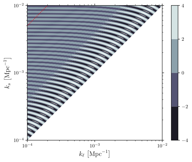
We are now in position to discuss what happens in the case of resonant non-Gaussianity: to have an idea of how the basis of operators should be augmented in this case, we need to determine how the long mode modifies the small-scale power spectrum. Let us start by considering the “ultra-squeezed” limit $k_{\ell}/k_{s}\ll 1/\alpha$, as opposed to the squeezed limit, $k_{\ell}/k_{s}\ll 1$. In this limit, the leading effect of the long mode on the short-scale power spectrum is equivalent to that of equilateral non-Gaussianity, as we can see from the CFC bispectrum of Eq. (18). That is, the small-scale power spectrum is modulated as in Eq. (20) with $\Delta=2$. However, things become more complicated as we take the long mode closer to $k_{s}/\alpha$. As we see from Fig. 2, for $k_{s}\ll 1/\alpha<k_{\ell}<k_{s}$ the response of the small-scale power spectrum to the long mode is made up of two contributions: a slowly-varying envelope and an oscillatory part. The oscillations are linear in $k_{\ell}$, and their frequency increases linearly with $\alpha$. Since the envelope is varying slowly with $k_{\ell}$, we can imagine that it will be described fully by an expansion of the form of Eq. (22). The same cannot be said about the oscillatory part: for it we also have a superposition of modulations of the form of Eq. (22) (starting from $\Delta=0$), but the coefficients $a_{0,2n}$ are now of order $\alpha^{2n}$: correspondingly, in the bias expansion we would have terms of the form

$$\delta_{h}\supset b_{\Psi^{(2n)}}\alpha^{2n}\Psi^{(2n)}\propto b_{\Psi^{(2n)}}\alpha^{2n}\partial^{2n}\zeta\,\,.$$

(33)

Therefore, from Eq. (23) we conclude that the bias expansion loses all predictive power due to the nontrivial behavior of the non-separable bispectrum in this model, since all terms beyond the ultra-squeezed limit become equally important.¹⁰¹⁰ 10 Notice that, as in the usual case, there will be also effects coming from the transfer function. We expect them to still scale as powers of $(k/k_{\text{eq}})^{2}$, i.e. without an enhancement at large $\alpha$, since they do not arise from the expansion of the bispectrum in the squeezed limit.

However it is still possible to make some progress if we make the strong assumption that halo formation is an exactly local function of the initial density field smoothed on the single scale $R_{\ast}$. This happens, e.g., if we consider microscopic models of halo abundance: in this case one makes a specific ansatz about how precisely the Lagrangian halo number density depends on the statistics of the small-scale modes, and then assumes that the same relation holds when primordial non-Gaussianity is included. Since now there is no restriction to scales $k\ll R_{\ast}^{-1}$, this approach does not rely on expanding the primordial bispectrum in the squeezed limit. We can think of this approach as a resummation of all the beyond-squeezed-limit contributions discussed above. This will give rise to a scale-dependent correction $\Delta b_{1}(k)$ to the linear bias $b_{1}$, i.e. $b_{1}\to b_{1}+\Delta b_{1}(k)$. For example, Ref. [67] derived this correction by applying a conditional mass function approach (see [68, 69] for related, previous approaches). The non-Gaussianity was taken into account by applying an Edgeworth expansion to the Gaussian PDF of the density field. Stopping the Edgeworth expansion at the bispectrum level, $\Delta b_{1}(k)$ is given by

$$\Delta b_{1}(k)=\bigg[b_{1}\delta_{\text{c}}+\frac{\partial\log{\cal F}^{(3)}_{\ast}}{\partial\log\sigma_{\ast}}\bigg]\frac{2{\cal F}^{(3)}_{\ast}(k)}{\mathcal{M}_{\ast}(k)}\,\,.$$

(34)

Here, the shape factor ${\cal F}^{(3)}_{\ast}$ is defined by (we drop the subscript $\ell$ on $k_{3}=k_{\ell}$ from now on)

$${\cal F}^{(3)}_{\ast}(k)=\frac{1}{4\sigma_{\ast}^{2}P_{\phi}(k)}\int\frac{\mathrm{d}^{3}k_{s}}{(2\pi)^{3}}\mathcal{M}_{\ast}(k_{1})\mathcal{M}_{\ast}(k_{2})B_{\phi}(k_{1},k_{2},k)\,\,,$$

(35)

with $\bm{k}_{1}=\bm{k}_{s}-\bm{k}/2$, $\bm{k}_{2}={-\bm{k}_{s}}-\bm{k}/2$, and $\mathcal{M}_{\ast}(k)$ is equal to

$$\mathcal{M}_{\ast}(k)\equiv\mathcal{M}(k)W_{\ast}(k)\,\,,\qquad\mathcal{M}(k)=\frac{2}{3}\frac{k^{2}T(k)D_{1}(z)}{\Omega_{\text{m}}H^{2}_{0}}\,\,.$$

(36)

Notice that in Eq. (34) we can assume that $\mathcal{M}_{\ast}(k)\approx\mathcal{M}(k)$: this is a good approximation as long as we look at correlations on scales $k\ll 1/R_{\ast}$ (since we have $W_{\ast}(k)\approx 1$ there).

Let us now investigate in more detail the meaning of Eqs. (34), (35). Using Eq. (35), we can define the initial local variance-field of the small-scale density on the scale $R_{\ast}$ in the presence of long-wavelength potential perturbations $\phi(\bm{k})$ as

$$\hat{\sigma}^{2}_{\ast}(\bm{q})\equiv\sigma^{2}_{\ast}\left[1+\int\frac{\mathrm{d}^{3}k}{(2\pi)^{3}}{\cal F}^{(3)}_{\ast}(k)\phi(\bm{k})e^{i\bm{k}\cdot\bm{q}}\right]\,\,.$$

(37)

The meaning of this local variance can be better understood if we look at Eq. (20). Indeed, $\hat{\sigma}^{2}_{\ast}(\bm{q})$ is the integral of the local power spectrum $P_{\phi}(\bm{k}_{s}|\bm{q})$ over $k_{s}$, weighted by $\mathcal{M}_{\ast}^{2}(k_{s})$: that is, we can write the local power spectrum as

$$P_{\phi}(\bm{k}_{s}|\bm{q})=\bigg[1+\int\frac{\mathrm{d}^{3}k}{(2\pi)^{3}}\mathcal{F}^{(3)}_{\ast}(k)\phi(\bm{k})e^{i\bm{k}\cdot\bm{q}}\bigg]P_{\phi}(k_{s})\,\,.$$

(38)

By comparing with Eq. (20), then, we see that the local power spectrum is now modulated by the operator $\int\frac{\mathrm{d}^{3}k}{(2\pi)^{3}}\mathcal{F}^{(3)}_{\ast}(k)\phi(\bm{k})e^{i\bm{k}\cdot\bm{q}}$, which must be then included in the bias expansion. We also notice that, using Eqs. (19), (22) at leading order in the squeezed limit, we have

$$\begin{split}{\cal F}^{(3)}_{\ast}(k)&=\frac{1}{4\sigma_{\ast}^{2}P_{\phi}(k)}\int\frac{\mathrm{d}^{3}k_{s}}{(2\pi)^{3}}\mathcal{M}_{\ast}(k_{1})\mathcal{M}_{\ast}(k_{2})B_{\phi}(k_{1},k_{2},k)\\ &\approx\frac{1}{4\sigma_{\ast}^{2}P_{\phi}(k)}\int\frac{\mathrm{d}^{3}k_{s}}{(2\pi)^{3}}\mathcal{M}_{\ast}^{2}(k_{s})\bigg[4a_{0,0}\bigg(\frac{k}{k_{s}}\bigg)^{\Delta}P_{\phi}(k_{s})P_{\phi}(k)\bigg]\\ &=\frac{a_{0,0}k^{\Delta}}{\sigma_{\ast}^{2}}\int\frac{\mathrm{d}^{3}k_{s}}{(2\pi)^{3}}k_{s}^{-\Delta}W^{2}_{\ast}(k_{s})P_{\text{m}}(k_{s})\\ &=a_{0,0}k^{\Delta}\frac{\sigma^{2}_{\ast,-\Delta/2}}{\sigma_{\ast}^{2}}\,\,,\end{split}$$

(39)

where $\Delta=2$. That is, the additional operator $\int\frac{\mathrm{d}^{3}k}{(2\pi)^{3}}\mathcal{F}^{(3)}_{\ast}(k)\phi(\bm{k})e^{i\bm{k}\cdot\bm{q}}$ becomes degenerate with $\partial^{2}\phi\sim\delta_{\text{m}}$, as expected.

Then, let us go back to a bispectrum of the form of Eq. (19), and let us focus on the leading order in the squeezed limit: then, the scale-dependent bias $\Delta b_{1}(k)$ would be given by (this is merely a rephrasing of $\delta_{h}\supset b_{\Psi^{(\Delta)}}\Psi^{(\Delta)}$)

$$\Delta b_{1}(k)|_{\Delta}=a_{0,0}b_{\Psi^{(\Delta)}}k^{\Delta}\mathcal{M}^{-1}(k)\,\,,$$

(40)

where $b_{\Psi^{(\Delta)}}$ is given by Eq. (29) for a mass function of the form of Eq. (25). At higher orders in the squeezed limit, we would have

$$\Delta b_{1}(k)|_{\Delta+2n}=a_{0,2n}b_{\Psi^{(\Delta+2n)}}k^{\Delta+2n}\mathcal{M}^{-1}(k)\,\,.$$

(41)

Therefore we see that the (scale-dependent) resummation of all the bias coefficients $b_{\Psi^{(\Delta+2n)}}$ becomes

$$\sum_{n=0}^{+\infty}a_{0,2n}b_{\Psi^{(\Delta+2n)}}k^{\Delta+2n}=\Delta b_{1}(k)\mathcal{M}(k)=\bigg[b_{\Psi^{(0)}}+4\bigg(\frac{\partial\log\big(\sigma^{2}_{\ast}{\cal F}^{(3)}_{\ast}(k)\big)}{\partial\log\sigma_{\ast}^{2}}-1\bigg)\bigg]{\cal F}^{(3)}_{\ast}(k)\,\,,$$

(42)

where ${\cal F}^{(3)}_{\ast}(k)$ is given by Eq. (35), and in the last equality we used Eq. (32). Ref. [67] showed that, for separable bispectrum shapes and for halos following a universal mass function, the leading squeezed-limit prediction of Eq. (34) agrees with Eq. (29). Moreover, Ref. [70] showed that this agreement also holds at the next-to-leading order in the squeezed-limit expansion. Finally, a more detailed proof of Eq. (42) and description of the resummation procedure are collected in Appendix B.

References

- (1) Planck Collaboration, P. A. R. Ade et al., “Planck 2015 results. XVII. Constraints on primordial non-Gaussianity,” Astron. Astrophys. 594 (2016) A17, arXiv:1502.01592 [astro-ph.CO].
- (2) M. Alvarez et al., “Testing Inflation with Large Scale Structure: Connecting Hopes with Reality,” arXiv:1412.4671 [astro-ph.CO].
- (3) T. Baldauf, M. Mirbabayi, M. Simonović, and M. Zaldarriaga, “Large-scale structure constraints with controlled theoretical uncertainties,” arXiv:1602.00674 [astro-ph.CO].
- (4) Y. Welling, D. van der Woude, and E. Pajer, “Lifting Primordial Non-Gaussianity Above the Noise,” JCAP 1608 no. 08, (2016) 044, arXiv:1605.06426 [astro-ph.CO].
- (5) J. Gleyzes, R. de Putter, D. Green, and O. Doré, “Biasing and the search for primordial non-Gaussianity beyond the local type,” JCAP 1704 no. 04, (2017) 002, arXiv:1612.06366 [astro-ph.CO].
- (6) S. Matarrese and L. Verde, “The effect of primordial non-Gaussianity on halo bias,” Astrophys. J. 677 (2008) L77–L80, arXiv:0801.4826 [astro-ph].
- (7) A. Slosar, C. Hirata, U. Seljak, S. Ho, and N. Padmanabhan, “Constraints on local primordial non-Gaussianity from large scale structure,” JCAP 0808 (2008) 031, arXiv:0805.3580 [astro-ph].
- (8) V. Desjacques and U. Seljak, “Primordial non-Gaussianity from the large scale structure,” Class. Quant. Grav. 27 (2010) 124011, arXiv:1003.5020 [astro-ph.CO].
- (9) V. Desjacques, D. Jeong, and F. Schmidt, “Large-Scale Galaxy Bias,” arXiv:1611.09787 [astro-ph.CO].
- (10) N. Dalal, O. Doré, D. Huterer, and A. Shirokov, “The imprints of primordial non-gaussianities on large-scale structure: scale dependent bias and abundance of virialized objects,” Phys. Rev. D77 (2008) 123514, arXiv:0710.4560 [astro-ph].
- (11) L. D. Ferramacho, M. G. Santos, M. J. Jarvis, and S. Camera, “Radio galaxy populations and the multitracer technique: pushing the limits on primordial non-Gaussianity,” Mon. Not. Roy. Astron. Soc. 442 no. 3, (2014) 2511–2518, arXiv:1402.2290 [astro-ph.CO].
- (12) D. Yamauchi, K. Takahashi, and M. Oguri, “Constraining primordial non-Gaussianity via a multitracer technique with surveys by Euclid and the Square Kilometre Array,” Phys. Rev. D90 no. 8, (2014) 083520, arXiv:1407.5453 [astro-ph.CO].
- (13) S. Ferraro and K. M. Smith, “Using large scale structure to measure and ,” Phys. Rev. D91 no. 4, (2015) 043506, arXiv:1408.3126 [astro-ph.CO].
- (14) A. Raccanelli, O. Doré, and N. Dalal, “Optimization of spectroscopic surveys for testing non-Gaussianity,” JCAP 1508 (2015) 034, arXiv:1409.1927 [astro-ph.CO].
- (15) R. de Putter and O. Doré, “Designing an Inflation Galaxy Survey: how to measure using scale-dependent galaxy bias,” Phys. Rev. D95 no. 12, (2017) 123513, arXiv:1412.3854 [astro-ph.CO].
- (16) E. Castorina, Y. Feng, U. Seljak, and F. Villaescusa-Navarro, “Primordial non-Gaussianities and zero bias tracers of the Large Scale Structure,” arXiv:1803.11539 [astro-ph.CO].
- (17) D. Karagiannis, A. Lazanu, M. Liguori, A. Raccanelli, N. Bartolo, and L. Verde, “Constraining Primordial non-Gaussianity with Bispectrum and Power Spectum from Upcoming Optical and Radio Surveys,” arXiv:1801.09280 [astro-ph.CO].
- (18) J. M. Maldacena, “Non-Gaussian features of primordial fluctuations in single field inflationary models,” JHEP 05 (2003) 013, arXiv:astro-ph/0210603 [astro-ph].
- (19) P. Creminelli and M. Zaldarriaga, “Single field consistency relation for the 3-point function,” JCAP 0410 (2004) 006, arXiv:astro-ph/0407059 [astro-ph].
- (20) E. Pajer, F. Schmidt, and M. Zaldarriaga, “The Observed Squeezed Limit of Cosmological Three-Point Functions,” Phys. Rev. D88 no. 8, (2013) 083502, arXiv:1305.0824 [astro-ph.CO].
- (21) L. Dai, E. Pajer, and F. Schmidt, “Conformal Fermi Coordinates,” JCAP 1511 no. 11, (2015) 043, arXiv:1502.02011 [gr-qc].
- (22) L. Dai, E. Pajer, and F. Schmidt, “On Separate Universes,” JCAP 1510 no. 10, (2015) 059, arXiv:1504.00351 [astro-ph.CO].
- (23) R. de Putter, O. Doré, and D. Green, “Is There Scale-Dependent Bias in Single-Field Inflation?,” JCAP 1510 no. 10, (2015) 024, arXiv:1504.05935 [astro-ph.CO].
- (24) T. Baldauf, U. Seljak, L. Senatore, and M. Zaldarriaga, “Galaxy Bias and non-Linear Structure Formation in General Relativity,” JCAP 1110 (2011) 031, arXiv:1106.5507 [astro-ph.CO].
- (25) C. Wagner, F. Schmidt, C.-T. Chiang, and E. Komatsu, “Separate Universe Simulations,” Mon. Not. Roy. Astron. Soc. 448 no. 1, (2015) L11–L15, arXiv:1409.6294 [astro-ph.CO].
- (26) T. Baldauf, U. Seljak, L. Senatore, and M. Zaldarriaga, “Linear response to long wavelength fluctuations using curvature simulations,” JCAP 1609 no. 09, (2016) 007, arXiv:1511.01465 [astro-ph.CO].
- (27) P. Creminelli, A. Perko, L. Senatore, M. Simonović, and G. Trevisan, “The Physical Squeezed Limit: Consistency Relations at Order ,” JCAP 1311 (2013) 015, arXiv:1307.0503 [astro-ph.CO].
- (28) E. Silverstein and A. Westphal, “Monodromy in the CMB: Gravity Waves and String Inflation,” Phys. Rev. D78 (2008) 106003, arXiv:0803.3085 [hep-th].
- (29) L. McAllister, E. Silverstein, and A. Westphal, “Gravity Waves and Linear Inflation from Axion Monodromy,” Phys. Rev. D82 (2010) 046003, arXiv:0808.0706 [hep-th].
- (30) R. Flauger, L. McAllister, E. Pajer, A. Westphal, and G. Xu, “Oscillations in the CMB from Axion Monodromy Inflation,” JCAP 1006 (2010) 009, arXiv:0907.2916 [hep-th].
- (31) R. Flauger and E. Pajer, “Resonant Non-Gaussianity,” JCAP 1101 (2011) 017, arXiv:1002.0833 [hep-th].
- (32) P. Creminelli, G. D’Amico, M. Musso, and J. Noreña, “The (not so) squeezed limit of the primordial 3-point function,” JCAP 1111 (2011) 038, arXiv:1106.1462 [astro-ph.CO].
- (33) S. R. Behbahani, A. Dymarsky, M. Mirbabayi, and L. Senatore, “(Small) Resonant non-Gaussianities: Signatures of a Discrete Shift Symmetry in the Effective Field Theory of Inflation,” JCAP 1212 (2012) 036, arXiv:1111.3373 [hep-th].
- (34) P. Creminelli, J. Noreña, M. Peña, and M. Simonović, “Khronon inflation,” JCAP 1211 (2012) 032, arXiv:1206.1083 [hep-th].
- (35) X. Chen and Y. Wang, “Quasi-Single Field Inflation and Non-Gaussianities,” JCAP 1004 (2010) 027, arXiv:0911.3380 [hep-th].
- (36) X. Chen and Y. Wang, “Quasi-Single Field Inflation with Large Mass,” JCAP 1209 (2012) 021, arXiv:1205.0160 [hep-th].
- (37) N. Arkani-Hamed and J. Maldacena, “Cosmological Collider Physics,” arXiv:1503.08043 [hep-th].
- (38) H. Lee, D. Baumann, and G. L. Pimentel, “Non-Gaussianity as a Particle Detector,” JHEP 12 (2016) 040, arXiv:1607.03735 [hep-th].
- (39) W. H. Kinney, “Horizon crossing and inflation with large eta,” Phys. Rev. D72 (2005) 023515, arXiv:gr-qc/0503017 [gr-qc].
- (40) M. H. Namjoo, H. Firouzjahi, and M. Sasaki, “Violation of non-Gaussianity consistency relation in a single field inflationary model,” EPL 101 no. 3, (2013) 39001, arXiv:1210.3692 [astro-ph.CO].
- (41) X. Chen, H. Firouzjahi, M. H. Namjoo, and M. Sasaki, “A Single Field Inflation Model with Large Local Non-Gaussianity,” EPL 102 no. 5, (2013) 59001, arXiv:1301.5699 [hep-th].
- (42) M. Akhshik, H. Firouzjahi, and S. Jazayeri, “Effective Field Theory of non-Attractor Inflation,” JCAP 1507 (2015) 048, arXiv:1501.01099 [hep-th].
- (43) S. Mooij and G. A. Palma, “Consistently violating the non-Gaussian consistency relation,” JCAP 1511 no. 11, (2015) 025, arXiv:1502.03458 [astro-ph.CO].
- (44) B. Finelli, G. Goon, E. Pajer, and L. Santoni, “Soft Theorems For Shift-Symmetric Cosmologies,” Phys. Rev. D97 no. 6, (2018) 063531, arXiv:1711.03737 [hep-th].
- (45) R. Bravo, S. Mooij, G. A. Palma, and B. Pradenas, “A generalized non-Gaussian consistency relation for single field inflation,” arXiv:1711.02680 [astro-ph.CO].
- (46) B. Finelli, G. Goon, E. Pajer, and L. Santoni, “The Effective Theory of Shift-Symmetric Cosmologies,” arXiv:1802.01580 [hep-th].
- (47) R. Bravo, S. Mooij, G. A. Palma, and B. Pradenas, “Vanishing of local non-Gaussianity in canonical single field inflation,” arXiv:1711.05290 [astro-ph.CO].
- (48) F.-Y. Cyr-Racine and F. Schmidt, “Oscillating Bispectra and Galaxy Clustering: A Novel Probe of Inflationary Physics with Large-Scale Structure,” Phys. Rev. D84 (2011) 083505, arXiv:1106.2806 [astro-ph.CO].
- (49) A. Moradinezhad Dizgah and C. Dvorkin, “Scale-Dependent Galaxy Bias from Massive Particles with Spin during Inflation,” JCAP 1801 no. 01, (2018) 010, arXiv:1708.06473 [astro-ph.CO].
- (50) G. Cabass, E. Pajer, and F. Schmidt, “How Gaussian can our Universe be?,” JCAP 1701 no. 01, (2017) 003, arXiv:1612.00033 [hep-th].
- (51) F. Schmidt and D. Jeong, “Cosmic Rulers,” Phys. Rev. D86 (2012) 083527, arXiv:1204.3625 [astro-ph.CO].
- (52) D. Jeong and F. Schmidt, “Cosmic Clocks,” Phys. Rev. D89 no. 4, (2014) 043519, arXiv:1305.1299 [astro-ph.CO].
- (53) D. Jeong and F. Schmidt, “Large-Scale Structure Observables in General Relativity,” Class. Quant. Grav. 32 no. 4, (2015) 044001, arXiv:1407.7979 [astro-ph.CO].
- (54) D. Bertacca, R. Maartens, and C. Clarkson, “Observed galaxy number counts on the lightcone up to second order: II. Derivation,” JCAP 1411 no. 11, (2014) 013, arXiv:1406.0319 [astro-ph.CO].
- (55) A. Kehagias, A. M. Dizgah, J. Noreña, H. Perrier, and A. Riotto, “A Consistency Relation for the Observed Galaxy Bispectrum and the Local non-Gaussianity from Relativistic Corrections,” JCAP 1508 no. 08, (2015) 018, arXiv:1503.04467 [astro-ph.CO].
- (56) E. Di Dio, H. Perrier, R. Durrer, G. Marozzi, A. M. Dizgah, J. Noreña, and A. Riotto, “Non-Gaussianities due to Relativistic Corrections to the Observed Galaxy Bispectrum,” JCAP 1703 no. 03, (2017) 006, arXiv:1611.03720 [astro-ph.CO].
- (57) A. Lewis, A. Challinor, and A. Lasenby, “Efficient computation of CMB anisotropies in closed FRW models,” Astrophys. J. 538 (2000) 473–476, arXiv:astro-ph/9911177 [astro-ph].
- (58) L. Boubekeur, P. Creminelli, J. Noreña, and F. Vernizzi, “Action approach to cosmological perturbations: the 2nd order metric in matter dominance,” JCAP 0808 (2008) 028, arXiv:0806.1016 [astro-ph].
- (59) P. D. Meerburg, “Oscillations in the Primordial Bispectrum I: Mode Expansion,” Phys. Rev. D82 (2010) 063517, arXiv:1006.2771 [astro-ph.CO].
- (60) Planck Collaboration, P. A. R. Ade et al., “Planck 2015 results. XX. Constraints on inflation,” Astron. Astrophys. 594 (2016) A20, arXiv:1502.02114 [astro-ph.CO].
- (61) BICEP2, Keck Array Collaboration, P. A. R. Ade et al., “Improved Constraints on Cosmology and Foregrounds from BICEP2 and Keck Array Cosmic Microwave Background Data with Inclusion of 95 GHz Band,” Phys. Rev. Lett. 116 (2016) 031302, arXiv:1510.09217 [astro-ph.CO].
- (62) T. Banks, M. Dine, P. J. Fox, and E. Gorbatov, “On the possibility of large axion decay constants,” JCAP 0306 (2003) 001, arXiv:hep-th/0303252 [hep-th].
- (63) P. Svrcek and E. Witten, “Axions In String Theory,” JHEP 06 (2006) 051, arXiv:hep-th/0605206 [hep-th].
- (64) M. Ballardini, F. Finelli, C. Fedeli, and L. Moscardini, “Probing primordial features with future galaxy surveys,” JCAP 1610 (2016) 041, arXiv:1606.03747 [astro-ph.CO]. [Erratum: JCAP1804,no.04,E01(2018)].
- (65) V. Assassi, D. Baumann, and F. Schmidt, “Galaxy Bias and Primordial Non-Gaussianity,” JCAP 1512 no. 12, (2015) 043, arXiv:1510.03723 [astro-ph.CO].
- (66) M. Biagetti, T. Lazeyras, T. Baldauf, V. Desjacques, and F. Schmidt, “Verifying the consistency relation for the scale-dependent bias from local primordial non-Gaussianity,” Mon. Not. Roy. Astron. Soc. 468 no. 3, (2017) 3277–3288, arXiv:1611.04901 [astro-ph.CO].
- (67) V. Desjacques, D. Jeong, and F. Schmidt, “Non-Gaussian Halo Bias Re-examined: Mass-dependent Amplitude from the Peak-Background Split and Thresholding,” Phys. Rev. D84 (2011) 063512, arXiv:1105.3628 [astro-ph.CO].
- (68) S. Matarrese, F. Lucchin, and S. A. Bonometto, “A path-integral approach to large-scale matter distribution originated by non-Gaussian fluctuations,” Astrophys. J. 310 (1986) L21–L26.
- (69) L. Verde and S. Matarrese, “Detectability of the effect of Inflationary non-Gaussianity on halo bias,” Astrophys. J. 706 (2009) L91–L95, arXiv:0909.3224 [astro-ph.CO].
- (70) F. Schmidt, “Non-Gaussian Halo Bias Beyond the Squeezed Limit,” Phys. Rev. D87 no. 12, (2013) 123518, arXiv:1304.1817 [astro-ph.CO].
- (71) A. L. Fitzpatrick, L. Senatore, and M. Zaldarriaga, “Contributions to the dark matter -Point function from the radiation era,” JCAP 1005 (2010) 004, arXiv:0902.2814 [astro-ph.CO].
- (72) Planck Collaboration, P. A. R. Ade et al., “Planck 2015 results. XIII. Cosmological parameters,” Astron. Astrophys. 594 (2016) A13, arXiv:1502.01589 [astro-ph.CO].
- (73) R. K. Sheth and G. Tormen, “Large scale bias and the peak background split,” Mon. Not. Roy. Astron. Soc. 308 (1999) 119, arXiv:astro-ph/9901122 [astro-ph].
- (74) D. J. Eisenstein and W. Hu, “Baryonic features in the matter transfer function,” Astrophys. J. 496 (1998) 605, arXiv:astro-ph/9709112 [astro-ph].
- (75) D. J. Eisenstein and W. Hu, “Power spectra for cold dark matter and its variants,” Astrophys. J. 511 (1997) 5, arXiv:astro-ph/9710252 [astro-ph].
- (76) F. Schmidt and M. Kamionkowski, “Halo Clustering with Non-Local Non-Gaussianity,” Phys. Rev. D82 (2010) 103002, arXiv:1008.0638 [astro-ph.CO].
- (77) A. Moradinezhad Dizgah, H. Lee, J. B. Muñoz, and C. Dvorkin, “Galaxy Bispectrum from Massive Spinning Particles,” arXiv:1801.07265 [astro-ph.CO].
- (78) F. Schmidt, N. E. Chisari, and C. Dvorkin, “Imprint of inflation on galaxy shape correlations,” JCAP 1510 no. 10, (2015) 032, arXiv:1506.02671 [astro-ph.CO].
- (79) N. E. Chisari, C. Dvorkin, F. Schmidt, and D. Spergel, “Multitracing Anisotropic Non-Gaussianity with Galaxy Shapes,” Phys. Rev. D94 no. 12, (2016) 123507, arXiv:1607.05232 [astro-ph.CO].
- (80) K. Kogai, T. Matsubara, A. J. Nishizawa, and Y. Urakawa, “Intrinsic galaxy alignment from anisotropic primordial non-Gaussianity,” arXiv:1804.06284 [astro-ph.CO].
- (81) A. S. Schmidt, S. D. M. White, F. Schmidt, and J. Stücker, “Cosmological N-Body Simulations with a Large-Scale Tidal Field,” arXiv:1803.03274 [astro-ph.CO].
- (82) D. Wands, K. A. Malik, D. H. Lyth, and A. R. Liddle, “A New approach to the evolution of cosmological perturbations on large scales,” Phys. Rev. D62 (2000) 043527, arXiv:astro-ph/0003278 [astro-ph].
- (83) C. Cheung, P. Creminelli, A. L. Fitzpatrick, J. Kaplan, and L. Senatore, “The Effective Field Theory of Inflation,” JHEP 03 (2008) 014, arXiv:0709.0293 [hep-th].
- (84) S. Weinberg, “Quantum contributions to cosmological correlations,” Phys. Rev. D72 (2005) 043514, arXiv:hep-th/0506236 [hep-th].
- (85) X. Tong, Y. Wang, and S. Zhou, “On the Effective Field Theory for Quasi-Single Field Inflation,” JCAP 1711 no. 11, (2017) 045, arXiv:1708.01709 [astro-ph.CO].