IUEP-HEP-18-02
Higgs-boson-pair production from gluon fusion at the HL-LHC and HL-100 TeV hadron collider
Abstract
We perform the most up-to-date comprehensive signal-background analysis for Higgs-pair production in channel at the HL-LHC and HL-100 TeV hadron collider, with the goal of probing the self-coupling of the Higgs boson which is normalized to its Standard Model value of . We simulate all the standard-model signal and background processes and emphasize that the background has been overlooked in previous studies. We find that even for the most promising channel at the HL-LHC with a luminosity of 3000 fb-1, the significance is still not high enough to establish the Higgs self-coupling at the standard model (SM) value. Instead, we can only constrain the self-coupling to at confidence level after considering the uncertainties associated with the top-Yukawa coupling and the estimation of backgrounds. Here we also extend the study to the HL-100 TeV hadron collider. With a luminosity of 3 ab-1, we find there exists a bulk region of in which one cannot pin down the trilinear coupling. Otherwise one can measure the coupling with a high precision. At the SM value, for example, we show that the coupling can be measured with about 20 % accuracy. While assuming 30 ab-1, the bulk region reduces to and the trilinear coupling can be measured with about 7 % accuracy at the SM value.
I Introduction
Origin of mass is the most important question that one would ask for our existence. This is related to the mechanism involved in electroweak symmetry breaking (EWSB), which is believed to give masses to gauge bosons and fermions. The simplest implementation in our standard model (SM) is to introduce a Higgs doublet field, whose non-vanishing vacuum expectation value causes EWSB [1]. The by-product is a neutral scalar Higgs boson, which was eventually discovered in July 2012 [2]. After accumulating enough data at the end of 8 TeV runs, the scalar boson is best described by the SM Higgs boson [3], in which the couplings to gauge bosons are confirmly established and those to fermions started to fall in the ball-park of the SM values. However, the SM Higgs boson can hardly constitute a complete theory because of, for example, the gauge hierarchy problem.
The current measurements of the Higgs-boson properties mainly concern the couplings of the Higgs boson to the SM particles. There is no a priori reason why the EWSB sector simply contains only one Higgs doublet field. Indeed, many extensions of the EWSB sector consist of more Higgs fields. Until now there is no information at all about the self-couplings of the Higgs boson, which depends on the dynamics of the EWSB sector. The self-couplings of the Higgs boson are very different among the SM, two-Higgs doublet models (2HDM), and MSSM. One of the probes of Higgs self-coupling is Higgs-boson-pair production at the LHC [4, 5, 6]. There have been a large number of works in literature on Higgs-pair production in the SM [7], in model-independent formalism [8], in models beyond the SM [9], and in SUSY [10].
The predictions for various models are largely different such that the production rates can give valuable information on the self-coupling . In the SM, Higgs-pair production receives contributions from both the triangle and box diagrams, which interfere with each other. It is only the triangle diagram that involves the Higgs self-trilinear coupling , yet the top-Yukawa coupling appears in both triangle and box diagrams. Therefore, we have to disentangle the triangle diagram from the box diagram in order to probe the Higgs trilinear coupling. In Ref. [11], we pointed out that the triangle diagram, with -channel Higgs propagator, is more important at low invariant-mass region than the box diagram. Thus, the Higgs-boson pair from the triangle diagram tends to have lower invariant mass, and therefore the opening angle in the decay products of each Higgs boson tends to be larger than that from the box diagram. Indeed, the opening angle separations and between the decay products of the Higgs-boson pair are very useful variables to disentangle the two sources. However, in Ref. [11] we only assumed some level of signal uncertainties to evaluate the sensitivity to the parameter space of self-coupling and the top-Yukawa coupling , without calculating all the other SM backgrounds, e.g., jet-fake backgrounds, single Higgs associated backgrounds, and non-resonant backgrounds.
In this work, we perform the most up-to-date comprehensive signal-background analysis for Higgs-pair production through gluon fusion and the decay channel. For other production and decay channels and some combined analyses, see Refs. [12]. We simulate the signal and all background processes using simulation tools as sophisticated as what experimentalists use. The signal subprocess is with various values for . The background includes , , single Higgs associated backgrounds (e.g. , , , followed by ), and non-resonant or jet-fake backgrounds (e.g. , , , , etc). We found a set of useful selection cuts to reduce the backgrounds. We express the sensitivity that can be achieved in terms of significance. We find that even for the most promising channel at the HL-LHC, the significance is still not high enough to establish the Higgs self-coupling at the SM value, though the self-coupling can be constrained to the range at confidence level (CL) with an integrated luminosity of 3000 fb-1. Taking account of the uncertainties associated with the top-Yukawa coupling and the estimation of backgrounds, we have found that the CL region broadens into . We also extend the analysis to the HL-100 TeV hadron collider. With a luminosity of 3 ab-1, we find a bulk region of in which one cannot pin down the trilinear coupling. Otherwise one can measure the coupling with a high precision. At the SM value, for example, we show that the coupling can be measured with about 20% accuracy. While assuming 30 ab-1, the bulk region reduces to and the trilinear coupling can be measured with about 7 % accuracy at the SM value. This is the main result of this work.
This work has a number of improvements over our previous and other works in literature, summarized as follows.
- 1.
We have included all the backgrounds, including related ones, single Higgs associated production processes, non-resonant backgrounds, and jet-fake backgrounds. Furthermore we would like to emphasize that we have implemented through detector simulations of all the backgrounds.
- 2.
While implementing all the relevant signal and background simulations, we find that the background is possibly very important and has been overlooked in previous studies. Note that the similar observation has been recently made by the authors of Ref. [13].
- 3.
For the signal, since the signal distributions behave differently for different , we evaluate the selection efficiency separately for each to properly cover the viable range of the non-standard values of .
- 4.
At the HL-LHC, we firstly take into account the impact of the uncertainty associated with the top-Yukawa coupling on CL sensitivity. We find that, especially, the lower boundary of the 95% CL region of significantly varies upon the expected precision of the top-quark Yukawa coupling in the HL-LHC era.
- 5.
Taking account of all the backgrounds known up to date and devising a new set of selection cuts, we have most reliably estimated the potential reach of HL-100 TeV hadron collider for a broad range of .
- 6.
At the HL-100 TeV collider, we find there is a two-fold ambiguity in which could be lifted up by exploiting several kinematical distributions. We also find that there exists a bulk region in which it would be difficult to establish the coupling even at the HL-100 TeV collider.
The organization is as follows. In the next section, we briefly describe the effective Lagrangian for Higgs-pair production. In Sec. III, we describe the signal and background processes and simulation tools. We also present the distributions, selection cuts, cut flows of signal and backgrounds, and significance for the HL-LHC. Section IV is dedicated to the case of HL-100 TeV hadron collider. In Sec. V, we examine the impact of the NLO corrections considering full top-quark mass dependence, the effect of using a modern PDF set to include the LHC data on PDF, and how the investigation of the uncertainties involved in the matching procedures affects the 95% CL sensitivity region of . We discuss and conclude in Sec. VI. We put some extra distributions and cut flow tables, which can be ignored in the first reading, into the appendices A and B. Appendix C, on the other hand, gives the details for the procedures employed in the matching in calculating the cross sections of the non-resonant backgrounds, as well as their uncertainties.
II Effective Lagrangian
The contributing Feynman diagrams for Higgs-boson-pair production via gluon fusion include a triangle diagram with a Higgs-boson propagator and a box diagram with colored particles running in them. The relevant couplings involved are top-Yukawa and the Higgs trilinear self coupling, which are given in this Lagrangian:
| (1) |
In the SM, . The differential cross section for the process was obtained in Ref. [14] as
| (2) |
where
| (3) |
and , , and with . The loop functions , , and with and given in Appendix A.1 of Ref. [14]. In the heavy quark limit, one may have
| (4) |
leading to large cancellation between the triangle and box diagrams.
The production cross section normalized to the corresponding SM cross section, with or without cuts, can be parameterized as follows:
| (5) |
where the numerical coefficients depend on and experimental selection cuts. Numerically, are at 14 TeV and at 100 TeV [11]. Upon our normalization, the ratio should be equal to when , or . The coefficients and are for the contributions from the triangle and box diagrams, respectively, and the coefficient for the interference between them. Once we have the coefficients the cross sections can be easily obtained for any combinations of couplings.
To get a feeling for the size of the cross sections that we are considering, we show the total production cross sections for various production channels in Fig. 1. At 14 TeV, the SM cross sections fb [15], fb [16], fb [17], and fb [16] are calculated at NNLO+NNLL, NLO, NNLO, and NLO, respectively [18]. The 100 TeV cross sections fb, fb, fb, and fb are calculated at the same orders as at 14 TeV [19, 20]. From Fig. 1, it is clear that the gluon fusion into gives the largest cross sections independently of with its minimum occurring at . From now on we shall focus on the gluon fusion mechanism. We show the ratio of the cross sections for the process as a function of in Fig. 2, in which we also indicate the effects of allowing the top-Yukawa coupling to have uncertainty or . At the HL-LHC, the expected precision of measurement of the top-quark Yukawa coupling is [21]. Currently, without knowing the absolute value of the top-quark Yukawa coupling no better than precision, we also consider the effect at 100 TeV though the expected uncertainty is at the 100-TeV colliders.
III Simulations, Event Selections, and Analysis at the 14 TeV HL-LHC
Our goal is to disentangle the effects of trilinear Higgs coupling, which is present in the triangle diagram, in Higgs-pair production. We focus on the decay channel , in which the final state consists of a pair of quarks and a pair of photons reconstructed at the invariant mass around the Higgs-boson mass ( GeV). We shall vary the value for the trilinear coupling between and to visualize the effects of . The backgrounds then include
- •
single-Higgs associated production, such as followed by ,
- •
non-resonant backgrounds and jet-fake backgrounds, such as , , , , , , and ,
- •
lepton) and lepton) backgrounds .
All the signal and backgrounds are summarized in Table 1, together with the information of the corresponding event generator, the cross section times the branching ratio (), the order in QCD for the calculation of , and the Parton Distribution Function (PDF) used.
| Signal | |||||
| Signal process | Generator/Parton Shower | [fb] | Order | PDF used | |
| in QCD | |||||
| [18] | / | 0.119 | NNLO | NNPDF2.3LO | |
| NNLL | |||||
| Backgrounds | |||||
| Background(BG) | Process | Generator/Parton Shower | [fb] | Order | PDF used |
| in QCD | |||||
| / | NNNLO | ||||
| Single-Higgs | / | 1.37 | NLO | ||
| associated BG [18] | / | 2.24 | NLO | ||
| / | 1.26 | NLO | |||
| Non-resonant BG | / | LO | |||
| / | LO | ||||
| / | LO | ||||
| / | LO | ||||
| / | LO | ||||
| / | LO | ||||
| / | LO | ||||
| and BG | [22] | / | NNLO | ||
| NNLL | |||||
| ( lepton) | [23] | / | NLO | ||
III.1 Parton-level event generations and detector simulations
Parton-level events for the backgrounds , , , , , , , and and for the signal with are generated with MadGraph5_aMC@NLO (MG5_aMC@NLO) [24]. Backgrounds for gluon fusion and top-quark pair are generated with POWHEG BOX [25]. The single-Higgs associated backgrounds for are generated with Pythia8 [26]. Here we would like to provide more detailed information on the parton-level generation of signal and background events. The signal cross sections are calculated with the adjustable Higgs self-coupling in UFO format [27] and events are generated in the loop induced mode [28]. The MadSpin code [29] is then employed to let the Higgs-boson pair decay into . Further on the parton-level generation of non-resonant and backgrounds, the following pre-selection cuts at parton level are imposed in order to avoid any divergence in the parton-level calculations [30]:
| (6) |
For parton showering, hadronization, and decays of unstable particles, Pythia8[26] is used both for signal and backgrounds. Finally, fast detector simulation and analysis at the HL-LHC are performed using Delphes3 [31] with the ATLAS template. In the template, we use the expected performance for photon efficiency, photon fake rates, -jet tagging efficiency, and -jet fake rates obtained with a mean pile-up (see Refs. [30, 32]). For the photon efficiency, we use the -dependent formula
which we obtain by fitting to the ATLAS simulation results. At , as in Ref. [30] and it approaches in the saturation region of the curve, at to be specific, being consistent with ATLAS simulation [32]. The photon fake rates are taken from Ref. [30]: and in the barrel (endcap) region. The -jet tagging efficiency depends on and of jet and we have fully considered its and dependence, see Fig.7(b) of Ref. [32]. The charm-jet fake rate depends on and, accordingly, on and of jet. For the multi-variate MV1 -tagging algorithm taken in our analysis, when and it approaches as [33]. In our simulation, the and dependence of is also considered. For the light-jet fake rate, we are taking [30]. Incidentally, we have also considered the energy loss due to the momentum reconstruction from the -tagged jet and set the jet-energy scale using the scaling formula [31]
where the factor 1.27 is tuned to get a correct peak position at in the invariant mass distribution of a -quark pair in the signal process.
In this study, we do not include the pile-up effects into our simulation. There are a couple of reasons for this. First, it is expected that the pile-up effects can be dealt with by the upgraded event trigger in future, and its overall effect could be negligible in the channel of our interests 11 1 It is shown that the rejection factor for pile-up jets could be 1350 with a mean pile-up [30]. According to ATLAS simulation, only and of jets identified as (sub)leading -jets and reconstructed (sub)leading photons, respectively, originate from pile-up jets. . More importantly, by imposing a narrow invariant mass window cut in event selection, we could eventually obtain similar results independently of including the pile-up effects. This is because pile-up causes the stronger impact on photons than on -jets and the soft fake photons from pile-up jets make the width of peak wider. Incidentally, we also have checked that the simulation results using the ATLAS -tagging efficiency in the presence of pile-up are similar to those obtained by using the -tagging efficiency in the absence of pile-up (the MV1 algorithm).
III.2 Signal Event Samples
The dominant mechanism for Higgs-pair production is the gluon fusion process at the hadron colliders. Other processes are more than an order of magnitude smaller. Thus, only the gluon fusion production mode is used for the signal process . These samples are generated with at LO 22 2 We use GeV.. They are showered by to model the parton showering and hadronization. Note that the A14 tune and the PDF [34] set are used together.
The signal event samples are generated with various self-coupling strengths in order to show their characteristics: with being corresponding to the SM Higgs self-coupling strength. And, the expected signal yields are normalized to the cross section computed at next-to-next-to-leading-order (NNLO) accuracy including next-to-next-to-leading-log (NNLL) gluon resummation [18] 33 3 For the signal event normalization, we take the cross section computed in the infinite top quark mass approximation [18]. . In Table 2, we show the production cross section times the branching ratio at the 14 TeV LHC for six selected values of . To obtain the production cross section for the non-SM values of , we have used44 4 See also Fig. 2.
| (7) |
| -4 | 0 | 1 | 2 | 6 | 10 | |
|---|---|---|---|---|---|---|
| [fb] | 1.45 | 0.25 | 0.12 | 0.06 | 0.48 | 1.97 |
III.3 Background Samples
The backgrounds mainly come from the processes with multiple jets and photons. They can mimic the signal-like two photons and two -jets in the final state. These backgrounds can be categorized into
- •
Single-Higgs associated backgrounds: , , and ,
- •
Non-resonant (continuum) backgrounds: , , , , , and events with an additional jet,
- •
and backgrounds in which at least one of the top quarks decays leptonically.
The information is summarized in Table 1.
III.3.1 Single-Higgs associated backgrounds
The gluon-fusion process is generated using POWHEG-BOX [25] and then the background yield is normalized using the cross section at next-to-next-to-next-leading order (NNNLO) in QCD [18]. The samples for , and are generated using and they are normalized to the cross sections calculated at NLO in QCD [18].
III.3.2 Non-resonant backgrounds
The non-resonant or continuum background (BG) processes included for the analysis are , , , , , and . They are all generated with and interfaced with for showering and hadronization, and the PDF [35] set is taken. Note that these samples are generated inclusively with an additional hard jet to capture the bulk of the NLO corrections. We then avoid the double counting problems in our non-resonant background samples by applying the pre-selection cuts listed in Eq. (6). We have found that the resulting cross sections for the non-resonant backgrounds, presented in Table I, agree with those presented in Ref. [30] within errors of less than 5%.
Among them, as will be shown, the and samples give the dominant BG yields. In the latter, is faking . The sub-dominant BGs come from the , , and processes with faking and/or faking . And the next sub-leading BG is from the sample. Here, one should be cautious about the process because it receives contributions not only from the light hard quarks and gluons but also from hard charm quarks. Schematically, one may write 55 5 For our analysis, first we have removed jet from a set of an additional hard jet.
| (8) | |||||
In the first line, 66 6 Here, denotes a light hard jet originating from light , , and quarks and gluons. Do not confuse it with which is for a hard jet originating not only from the light quarks and gluons but also from quarks. in the first bracket denotes the additional light hard jet and in the last bracket is for jets generated during the showering process or , etc with the subscript standing for showering jets. In the second line, we use with the subscript standing for jets from hard scatterings. We definitely see that the first part of Eq. (8) constitutes a part of the sample and should be removed from the sample to avoid a double counting. After removing it, we find that the process with dominates the BG with faking . Note that charm quarks should be treated separately from the light quarks since the -quark fake rate is much larger than the light-jet fake rate of . Incidentally, we recall that . Finally, the sample has the least contribution to the non-resonant backgrounds. In Table 3, we are summarizing the main fake processes and rates in each sample of backgrounds.
| Background(BG) | Process | Fake Process | Fake rate |
|---|---|---|---|
| Non-resonant | N/A | N/A | |
| , | |||
| , | |||
| BG | , , | ||
| , | |||
| N/A | N/A | ||
| Leptonic decay | , | // | |
| Semi-leptonic decay | , | / | |
| Leptonic decay | / | ||
| Semi-leptonic | / |
III.3.3 and backgrounds
The background is generated at NLO in QCD using POWHEG-BOX, and interfaced to for parton showering and hadronization. And for the PDF set, [36] is taken. Since it mimics the signal with an electron in the final state faking a photon, we have required the final state should include at least lepton 77 7 Here a lepton means , , or .. And the BG yield is normalized using the cross section calculated with program at NNLO in QCD which also includes soft-gluon resummation to NNLL [22]. Here we are taking GeV.
A background with a similar size comes from the production with one photon in the final state. The sample is generated at LO in QCD with and interfaced with for showering and hadronization. For , we are taking the PDF set and the BG yield is normalized using the cross section calculated in NLO in QCD [23]. Also, as in , we require the final state to contain at least lepton. In Table 3, we are summarizing the main fake processes and rates also for the and backgrounds.
| Sequence | Event Selection Criteria at the HL-LHC |
|---|---|
| 1 | Di-photon trigger condition, 2 isolated photons with GeV, |
| 2 | 2 isolated photons with GeV, or , |
| 3 | 2 jets identified as b-jets with leading(sub-leading) GeV, |
| 4 | Events are required to contain jets with GeV within |
| 5 | No isolated leptons with GeV, |
| 6 | , |
| 7 | and |
| 8 | GeV, GeV |


III.4 Event Selections
A sequence of event selections is applied to the signal and background samples. It is clearly listed in Table 4. We follow closely the steps reported in an ATLAS conference report [30]. The goal is to obtain a pair of isolated photons and a pair of isolated quarks. Both pairs are reconstructed near the Higgs-boson mass. In particular, the cuts and are imposed so as to suppress the main backgrounds which are more populated in the regions of , see Fig. 3 88 8 For larger values of , the cuts of remove more signal events compared to the SM case, see the upper left frame of Fig. 13 in Appendix A. This leads to the smaller efficiencies as shown in Table 5 when , , and . We find that the different choices of cuts hardly improve the signal significance and employ the same cuts taken by the ATLAS group [30]. . We show the angular separation between photons and that between jets for all the backgrounds and the signal with in the left and right frame of Fig. 3, respectively. It is clear that the majority of the signal and a very few backgrounds lie in the region and . In Fig. 4, we show the transverse momentum distributions and for the signal with and all the backgrounds. We observe the signal tends to have larger transverse momentum. Distributions of and with other values of can be found in Appendix A where we also show the and distributions. The details of cuts are summarized in Table 4.
All events passing the above selection criteria are classified into two categories, depending on the pseudorapidities of the photons. If both photons appear in the barrel region () the event is labeled as “barrel-barrel”, otherwise it is labeled as “other”.
| 0 | 1 | 2 | 6 | 10 | ||||||||
| Cross section (fb) | 1.45 | 0.25 | 0.12 | 0.06 | 0.48 | 1.97 | ||||||
| Cuts | Eff. | No. | No. | No. | ||||||||
| 1. diphoton trigger | 23.15 | 1007 | 25.63 | 192 | 27.47 | 99 | 28.94 | 52 | 20.50 | 295 | 21.01 | 1242 |
| 2. isolated photons | 20.79 | 904 | 23.33 | 175 | 25.21 | 91 | 26.73 | 48 | 17.82 | 257 | 18.38 | 1086 |
| 3-1. jet candidates | 14.58 | 634 | 17.10 | 128 | 19.07 | 69 | 20.85 | 38 | 11.62 | 167 | 12.14 | 717 |
| 3-2 two b-jet | 4.61 | 200 | 5.65 | 42 | 6.46 | 23 | 7.26 | 13 | 3.34 | 48 | 3.55 | 210 |
| 4. no. of jets | 4.47 | 194 | 5.43 | 41 | 6.23 | 22 | 6.97 | 13 | 3.26 | 47 | 3.45 | 204 |
| 5. lepton veto | 4.41 | 192 | 5.36 | 40 | 6.15 | 22 | 6.88 | 12 | 3.22 | 46 | 3.41 | 202 |
| 6. cut | 2.72 | 118 | 4.00 | 30 | 4.98 | 18 | 5.87 | 11 | 1.19 | 17 | 1.49 | 88 |
| 7-1. Higgs mass window | 2.65 | 115 | 3.88 | 29 | 4.82 | 17 | 5.64 | 10 | 1.15 | 17 | 1.46 | 86 |
| 7-2. Higgs mass window | 1.80 | 78 | 2.62 | 20 | 3.20 | 12 | 3.82 | 7 | 0.78 | 11 | 0.99 | 59 |
| 8. cuts | 1.77 | 77 | 2.60 | 20 | 3.17 | 11 | 3.79 | 7 | 0.77 | 11 | 0.97 | 57 |
| other/barrel ratio | 35.27 % | 36.08% | 33.89% | 32.66% | 39.47% | 37.01% | ||||||
III.5 Cut Flows and Efficiencies
We follow closely the steps used in the ATLAS conference note [30]. We compare the cut flow of our current analysis with ATLAS results for the case, and they agree with each other within about 5–15%. We show in Table 5 the efficiencies and event yields for Higgs-pair production in the channel at the HL-LHC with an integrated luminosity of 3000 fb-1 for various values of . In the last row, “other/barrel ratio” is the ratio of events for the two photon candidates falling in the “other” region to those in the “barrel-barrel” region, after applying all the event selection cuts. The overall other/barrel ratios are all similar.
The overall signal efficiency has its peak value of 3.79 % at and it decreases when deviates from . We observe that the overall efficiency drops quickly when moves to a larger value and becomes smaller than 1 % when . While when becomes smaller and starts to take on negative values, it decreases to 3.17 % at the SM value of and reaches 1.77 % at . This is because of the strong destructive (constructive) interference between the triangle and box diagrams for the positive (negative) values of and the enhancement of kinematical features of the triangle diagram for . Thus, these two effects are combined to give strong dependence of the distributions on , and therefore leading to the strong dependence of the signal efficiency on . On the other hand, the number of signal events, which is given by the product of the cross section, signal efficiency, and luminosity of 3000 fb-1, is only 7 at but it becomes 11 at the SM value of . Note that one may have the same number of signal events also at .
The cut flow tables of all the backgrounds in terms of efficiencies at the HL-LHC are presented in Appendix B.
| Expected yields | Total | Barrel-barrel | Other | Ratio (O/B) | of Gen. |
| Samples | (End-cap) | Events | |||
| , | |||||
| , | |||||
| , | |||||
| , | |||||
| , | |||||
| , | |||||
| ( 1 leptons) | |||||
| ( 1 leptons) | |||||
| Total Background | |||||
| Significance | |||||
| Combined significance | |||||
III.6 Analysis and Results
Here we show the main results of our analysis in Table 6 – the resultant signal rates for various against all the backgrounds. The last column is for the number of generated events in each sample. The statistical uncertainties originating from the limited number of generated events are estimated by dividing each of the background and signal samples into roughly subsamples. The fluctuations among the subsamples are then taken as the uncertainty of the sample. We have made detailed comparisons with the results from ATLAS [30]. In general we agree, except for and . In the sample, we figure out that about half of the disagreement is caused by the differences in -tagging algorithm and detector simulations. While, for the sample, our estimation is made based on the Delphes3 algorithm for electron reconstruction and identification which is about 20 times more efficient than that taken by ATLAS.
More precisely, in the sample, our number of the background is which is times larger than the ATLAS number of [30]. By noting that the sample is dominated by quarks from showering processes, we find a part of the difference can be attributed to different -tagging algorithm taken in our work: ours is from [32] while, in the ATLAS paper, the algorithm from [37] is used. If we use the same algorithm taken in the ATLAS paper, we find the number of background reduces to about which is still a bit above the ATLAS number . We also find another reason in the detector simulations but, again, it is not enough to fully explain the difference. Indeed, the similar observation has been recently made by the authors of Ref. [13]. When they used the same selection cuts as ATLAS, the result was also larger than the ATLAS result, but consistent with ours.
We note that the kinematic distributions for the signal with different would not be very different, as seen by the ratio in the last of Table 6, which are more or less the same for different . On the other hand, the ratio for the backgrounds, on average, is larger than the signal, which means the backgrounds are in general more forward. We further note that the combined significance obtained by splitting events into two categories of barrel-barrel and other is improved by 3 % over the total one when . For our analysis, we use the combined significance.
The most dominant one in the single-Higgs associated backgrounds is followed by . The single-Higgs associated processes contribute about 23 events to the total background. Meanwhile the dominant ones in non-resonant backgrounds are and with each of it contributing 19 events to the total background. A similar size of background comes from combined , in which either hard or showering quarks are faking jets basically. Among the non-resonant backgrounds, contributes the least. Including and in which one or two electrons are faking photons, we note that more than one half of the total background is due to fakes.


In Fig. 5, we show the resultant invariant-mass distributions of the two photon (upper) and two (lower) candidates for the signal on top of all the backgrounds. We have applied all the selection cuts except for the cut on () in the upper (lower) frame. The photon peak GeV is very clear while that of GeV is rather broad, due to the -jet resolution.
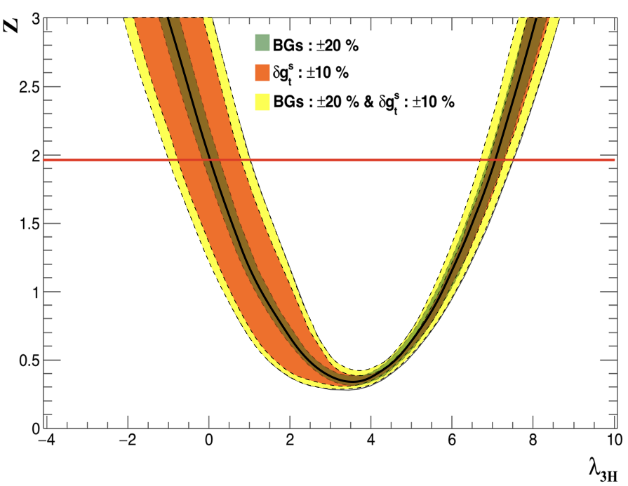
In Fig. 6, we show the significance defined by
| (9) |
where and represent the numbers of signal and background events, respectively. The central curve is for the case when the top-Yukawa coupling takes on the SM value of and , see Table 6. The orange and green bands have been obtained by varying the top-Yukawa coupling by 10 % 99 9 In our work, we also take account of the effect of the 10 % uncertainty of the top-Yukawa coupling on the and backgrounds while neglecting its effect on the Higgs decay mode into two photons since it is dominated by the loops. Incidentally, we have taken the SM values for the Higgs couplings to quarks and bosons for . () and the total background yield by 20 % (), respectively. The yellow band has been obtained by considering both of the uncertainties simultaneously. The uncertainty associated with the estimation of backgrounds may arise from pile-up, the photon and -tagging efficiencies, several fake rates, the choices of renormalization and factorizations scales and PDF, etc. We note that the effect becomes larger when decreases from . For , the effect could be comparably important. Given all the uncertainties can be minimized and the top-Yukawa at the SM value, the 95% CL sensitivity region for is . However, given the worst uncertainties with and , the sensitivity range widens to . We note that the lower boundary of the 95% CL region of is sensitive to the top-Yukawa while the impact of the uncertainty associated with the estimation of backgrounds turns out minor upon the 20 % variation over the total background.
Finally, we show in Fig. 7 the luminosity required to achieve 95% CL sensitivity versus . We observe that the SM value of can only be established with about 8.5 ab-1 luminosity. Note that the required luminosity peaks at while the production takes its smallest value at , see Fig. 1. This is because of the strong dependence of the signal efficiency on induced by the substantial interference between the triangle and box diagrams together with, especially for , the enhancement of kinematical features of the triangle diagram or the smaller Higgs-pair invariant mass of , the wider angular separations of , and the smaller transverse momenta of .
IV Simulations, Event Selections, and Analysis at the HL-100 TeV Collider
In this section, through the channel, we estimate how well one can measure the coupling at a 100 TeV hadron collider assuming a nominal luminosity of 3 ab-1 or at the HL-100 TeV hadron collider. We basically follow the procedures that we took in the last section for the 14 TeV HL-LHC case, though some selection cuts may be changed because of the much higher center-of-mass energy. We have taken a crude estimate projected from the current LHC detectors for the and coverage for jets, leptons, and photons without any specific detector designs available for the 100 TeV hadron collider.
IV.1 Parton-level event generations and detector simulations
| Signal | |||||
| Signal process | Generator/Parton Shower | [fb] | Order | PDF used | |
| in QCD | |||||
| [20] | / | 4.62 | NNLO | NNPDF2.3LO | |
| NNLL | |||||
| Backgrounds | |||||
| Background(BG) | Process | Generator/Parton Shower | [fb] | Order | PDF used |
| in QCD | |||||
| [20] | / | ||||
| Single-Higgs | [20] | / | NLO | ||
| associated BG | [20] | / | NNLO | ||
| [38] | / | NNLO(5FS) | |||
| Non-resonant BG | / | LO | |||
| / | LO | ||||
| / | LO | ||||
| / | LO | ||||
| / | LO | ||||
| / | LO | ||||
| / | LO | ||||
| and BG [20] | / | NLO | |||
| ( lepton) | / | NLO | |||
The same signal and backgrounds are considered as in the 14 TeV case. The Monte Carlo generators, the cross sections, and the orders of QCD calculation are shown in Table 7. Note that, for some backgrounds, the orders in QCD are different compared to the 14 TeV case. Otherwise, the calculational methods taken for the signal and background samples are essentially the same as those what we employed for the HL-LHC.
On the other hand, pre-selection cuts, detector energy resolutions, and tagging efficiencies and fake rates may undergo significant changes because of different designs and projected performance of the detectors in the future. Below, we describe in detail what we use in our analysis.
- •
Pre-selection cuts, which are imposed in order to avoid any divergence in the parton- level calculations, are modified as follows to match the wider coverage of future particle detectors:
- •
Fast detector simulation and analysis at the HL-100 TeV hadron collider are performed using Delphes3 [31] with the FCChh template. For the energy resolution of the detector, we have chosen the “Medium” detector performance for ECAL and HCAL [20] 1010 10 In Ref. [20], three scenarios of ECAL and HCAL performance are considered: “Low”, “Medium”, and “High”. because we could get the best significance for this choice. In the “Medium” performance scenario, the ECAL energy resolution is given by
and the HCAL energy resolution by
Further we set the magnetic field 6 T and the jet energy scale of is taken to get the correct peak position at in the invariant mass distribution of the -quark pair in the signal process.
- •
For the -jet tagging efficiency and related jet fake rates, we are taking %, %, and % [20].
- •
IV.2 Signal Event Samples
The signal event samples are generated in exactly the same way as in the HL-LHC case. We show the production cross section times the branching ratio at the 100 TeV collider for six selected values of in Table 8.
| -4 | 0 | 1 | 2 | 6 | 10 | |
|---|---|---|---|---|---|---|
| [fb] | 46.97 | 8.99 | 4.62 | 2.32 | 13.61 | 57.78 |
IV.3 Background Samples
As in the HL-LHC case, we categorize the backgrounds into single-Higgs associated backgrounds, non-resonant backgrounds, and and backgrounds. The information is summarized in Table 7. Note that the sample is generated with , and for showering, hadronization and decays of unstable particles only is used 1111 11 Note is used for the process at the HL-LHC.. Otherwise, the descriptions of the backgrounds are the same as in the HL-LHC case.
The cross sections increase as we move from 14 TeV to 100 TeV. The signal cross section increases by a factor of about . The cross section for the single-Higgs associated backgrounds increases by a factor of about except : the increment factor for the process is about . The cross section for the process increases by a factor of about while the increment factor of the other non-resonant backgrounds is about . The cross sections for the related backgrounds increase by about times. As we will show, the non-resonant backgrounds constitutes more than 75 % of the total backgrounds. Roughly, the cross sections for the signal and dominant background processes increase by a factor of about . Finally, in Table 9, we summarize the faking rates of non-resonant and -related backgrounds which we use for the HL-100 TeV collider.
| Background(BG) | Process | Fake Process | Fake rate |
|---|---|---|---|
| Non-resonant | N/A | N/A | |
| , | |||
| , | |||
| BG | , , | ||
| , | |||
| N/A | N/A | ||
| Leptonic decay | , | // | |
| Semi-leptonic decay | , | / | |
| Leptonic decay | / | ||
| Semi-leptonic | / |
| Sequence | Event Selection Criteria at the HL-100 TeV hadron collider |
|---|---|
| 1 | Di-photon trigger condition, 2 isolated photons with GeV, |
| 2 | 2 isolated photons with GeV, , |
| 3 | 2 jets identified as b-jets with leading(sub-leading) GeV, |
| 4 | Events are required to contain jets with GeV within |
| 5 | No isolated leptons with GeV, |
| 6 | , |
| 7 | and |
| 8 | GeV, GeV |
IV.4 Event Selections
A sequence of event selections is applied to the signal and background samples, see Table 10. We basically follow our HL-LHC analysis but using more relaxed condition to inclusively cover the broad range of still allowed after the HL-LHC era. Also considered are the wider coverage at 100 TeV and the more energetic jets and photons.
The distributions in , , , , , and are very similar to the case of HL-LHC. We collect some of them in appendix A in order not to interrupt smooth reading of the main text.
| 0 | 1 | 2 | 6 | 10 | ||||||||
| Cross section (fb) | 46.97 | 8.99 | 4.62 | 2.32 | 13.61 | 57.78 | ||||||
| Cuts | Eff. | No. | No. | No. | ||||||||
| 1. diphoton trigger | 56.06 | 78988 | 57.78 | 15582 | 58.99 | 8176 | 60.00 | 4176 | 53.44 | 21818 | 53.82 | 93293 |
| 2. isolated photons | 36.31 | 51158 | 39.21 | 10575 | 41.29 | 5722 | 43.40 | 3021 | 32.39 | 13225 | 32.94 | 57105 |
| 3-1. jet candidates | 29.07 | 40965 | 32.77 | 8838 | 35.36 | 4901 | 37.94 | 2641 | 23.87 | 9746 | 24.74 | 42881 |
| 3-2 two b-jet | 9.57 | 13492 | 11.41 | 3076 | 12.75 | 1767 | 14.18 | 987 | 7.31 | 2986 | 7.65 | 13252 |
| 4. no. of jets | 9.03 | 12724 | 10.60 | 2860 | 11.79 | 1634 | 13.04 | 907 | 6.99 | 2856 | 7.29 | 12638 |
| 5. lepton veto | 9.03 | 12724 | 10.60 | 2860 | 11.79 | 1634 | 13.04 | 907 | 6.99 | 2856 | 7.29 | 12637 |
| 6. cut | 8.32 | 11730 | 10.08 | 2718 | 11.34 | 1572 | 12.57 | 875 | 5.92 | 2419 | 6.39 | 11023 |
| 7-1. Higgs mass window | 7.78 | 10968 | 9.35 | 2523 | 10.51 | 1456 | 11.57 | 805 | 5.55 | 2268 | 5.97 | 10341 |
| 7-2. Higgs mass window | 6.14 | 8650 | 7.32 | 1974 | 8.23 | 1140 | 9.08 | 632 | 4.48 | 1830 | 4.77 | 8264 |
| 8. cuts | 3.98 | 5604 | 5.61 | 1514 | 6.79 | 941 | 8.01 | 557 | 1.84 | 753 | 2.21 | 3838 |
| other/barrel ratio | 31.64% | 30.14% | 30.05% | 29.18% | 33.03% | 31.26% | ||||||
IV.5 Cut Flows and Efficiencies
We closely follow the procedures that we employed for the HL-LHC. We show in Table 11 the efficiencies and event yields for Higgs-pair production in the channel with and an integrated luminosity of 3000 fb-1 at the 100 TeV collider.
The overall signal efficiency has its peak value of 8.01 % at and its behavior is similar to that at 14 TeV with % when , 6.79 % at the SM value of , and 3.98 % at . On the other hand, the number of signal event is 557 at and it becomes 941 at the SM value of . Note that one may have a similar number of signal events at .
The cut flow table of all the backgrounds in terms of efficiencies at the HL-100 TeV hadron collider is presented in Appendix B.
IV.6 Analysis and Results
| Expected yields | Total | Barrel-barrel | Other | Ratio (O/B) | of Gen. |
| Samples | (End-cap) | Events | |||
| , | |||||
| , | |||||
| , | |||||
| , | |||||
| , | |||||
| , | |||||
| ( 1 leptons) | |||||
| ( 1 leptons) | |||||
| Total Background | |||||
| Significance | |||||
| Combined significance | |||||
Here we show the main results of the analysis for the 100 TeV hadron collider, see Table 12. Among the single-Higgs associated backgrounds, the major ones come from and , comprising about 20 % of the total background. Meanwhile the dominant ones in non-resonant backgrounds are followed which make up about 60 % of the total background. Including other backgrounds, we note that 70 % of the total background is due to fakes. Being contrary to the HL-LHC case, the combined significance achieved is much higher: at the SM value of , which is mainly because of much higher signal event rates though the signal to background ratios are similar at HL-LHC and HL-100 TeV collider.


In Fig. 8, we show the resultant invariant-mass distributions of the two photon (upper) and two (lower) candidates for the signal on top of all the backgrounds at the HL-100 TeV collider, as similar to HL-LHC in Fig. 5. We observe the similar behavior as in the HL-LHC case.


Since the achieved significance is high enough, we try to estimate how well one can measure the coupling at the HL-100 TeV hadron collider. In the left frame of Fig. 9, we show the number of signal events as a function of . To obtain the curve we assume the luminosity of 3 ab-1 and take into account the -dependent overall signal efficiencies, see Table 11. One may find the values of for some representative choices of in Table 12. On the other hand, the solid horizontal line shows the number of signal events , as an example, when the input value of or takes the SM value of 1. The dotted lines delimit the 1- region considering the statistical error of with . For this purpose, we generate another pseudo dataset for the signal. By locating the points where the curve and the horizontal lines meet, one can obtain the two center values of output and the corresponding two regions of 1- error. Note that, usually, there is a two-fold ambiguity in this approach. By repeating this procedure for different input values of , we can obtain the center output values together with the regions of 1- error, as shown in the right frame of Fig. 9.
The black-shaded region (delimited by the black dashed lines) in the right frame of Fig. 9 shows the 1- errors versus the input values of with the luminosity of 3 ab-1. Incidentally, the black solid line shows the center values of output values or along the line denoted by the thin dotted line. We note that there exists a bulk region of in which one cannot pin down the coupling. We find that the bulk region reduces to assuming the luminosity of 30 ab-1 as shown by the red-shaded region (delimited by the red dashed lines) in the same frame of Fig. 9.
Even though it would be difficult to pin down the coupling in the bulk region, yet one goes a bit away from it and is able to measure the coupling with a high precision as indicated by the narrowness of the 1- error regions. And, the two-fold ambiguity can be lifted up by exploiting the kinematical differences found in the distributions of , , when takes on different values: see Fig. 15. Keeping these all in mind, in Fig. 10, we show the regions in which one can determine the coupling within an absolute error of (either upper or lower error) along the line assuming 3 ab-1 (upper panel) and 30 ab-1 (lower panel). The green-shaded regions around denote the bulk regions. We observe that, when or , one can pin down the coupling with an absolute error smaller than assuming ab-1. At the SM value of , specifically, we observe that the coupling can be measured with about % accuracy assuming the integrated luminosity of ab-1. Our results are about 2 times better than those reported in Ref. [39] and comparable with those in Ref. [40] taking account of the more sophisticated and comprehensive treatment of the background processes taken in this work.
Before moving to the next Section, we would like to comment that the bulk region can be shifted by adopting a different set of selection cuts and it may help if it turns out that falls into the bulk region in future.
V Further Improvements Envisaged
In our analysis, we are taking the SM cross sections of fb and fb at 14 TeV and 100 TeV, respectively, which are calculated at NNLO accuracy including NNLL gluon resummation in the infinite top quark mass approximation. We have taken these values of cross sections to confirm, especially, the ATLAS results [30]. Recently, the NLO corrections considering full top-quark mass dependence have been available [41, 42]. The calculation reveals that the full top-quark mass dependence is vital to get reliable predictions for Higgs boson pair production. Precisely, the total cross section is reduced by 14 % at 14 TeV compared to that obtained by the Born improved Higgs Effective Field Theory (HEFT) in which the infinite top mass approximation is taken. At 100 TeV, the larger reduction of 24 % is found.


At the moment, as suggested in Ref. [43], the best way to incorporate the finite top-quark mass effects at NNLO might be by adopting the FT approximation [16, 44] in which the full top-quark mass dependence is considered only in the real radiation while the HEFT is taken in the virtual part. At NNLO in the FT approximation, fb and fb at 14 TeV and 100 TeV, respectively [43]. We observe that 20 (30) % reduction at 14 (100) TeV compared to the cross sections used in Sections III and IV. To see the impact of the reduced cross sections on our main results, in Fig. 11, we show the signal significance over the background versus at the HL-LHC (left) and the regions in which one can determine the coupling with an absolute error of at the HL-100 TeV collider (right). At 14 TeV with 3000 fb-1, the trilinear coupling is constrained to be at 95% CL taking account of the uncertainties associated with the top-Yukawa coupling and the estimation of backgrounds. Taking the central line, the 95% CL sensitivity region for is which becomes broader by the amount of compared to the results presented in Section III 1212 12 Recall that the corresponding region is if the NNLO+NNLL cross section of 45.05 fb is taken.. At 100 TeV, we find a little bit broader bulk regions of and with 3 ab-1 and 30 ab-1, respectively, compared to the results presented in Section IV 1313 13 Recall that, when the NNLO+NNLL cross section of 1749 fb is taken at 100 TeV, the bulk regions are and can be measured with an accuracy of 20 (7) % at its SM value with 3 ab-1 (30 ab-1).. And, can be measured with an accuracy of 30 (10) % with an integrated luminosity of 3 (30) ab-1 when it takes on its SM value of . We observe that the effects of the reduced cross sections are less significant in the case with 30 ab-1 at 100 TeV in which the number of signal events is comparable to or larger than that of backgrounds.
The QCD corrections also affect the ratio which is used to obtain the cross sections for non-SM values of . The QCD corrections depend on and become larger when deviates from the SM value due to the nontrivial interference between the triangle and box diagrams [42]. We observe that the ratio increases by about 10 (35) % at , see Fig. 12. It is clear that the QCD corrections are less significant than the uncertainties associated with the top-Yukawa coupling, see Fig. 2. In this respect, we have not taken account of the -dependent QCD corrections on the ratio in this work 1414 14 Taking account of the -dependent QCD corrections, at 14 TeV, we observe that the central 95% CL sensitivity region reduces from to since the QCD corrections enhance the signal cross section for and .. On the other hand, when is significantly larger than , vertex corrections proportional to appear at the amplitude level. This may bring sizeable distortion to . In this case, it might be practical to consider as an effective parameter, not as a fundamental one.
Note that the and distributions are affected by the QCD corrections at NLO and NNLO as shown in, for example, Refs. [42, 43]. For more precise predictions at the HL-LHC and HL-100 TeV collider and to lift up the two-fold ambiguity in especially, one may need to incorporate them in the future.
The PDF set of CTEQ6L1 taken to calculate the non-resonant backgrounds does not include the use of data from LHC experiments. To study the impact of the LHC data on PDF, instead of CTEQ6L1, we take the PDF set of CT14LO [45] and re-simulate all the non-resonant backgrounds at 14 TeV. Taking the example of background, which is one of the two most severe non-resonant backgrounds, we obtain the overall efficiency of by generating events. This is very similar to the efficiency of obtained using CTEQ6L1, see Table 13. Actually, we observe that the two efficiencies in each step of cut flow coincide within less than 10% and there are no significant differences in kinematic distributions caused by CT14LO. Meanwhile, the real effect of CT14LO is the reduction of the cross sections for the non-resonant backgrounds. For , as an example, it reduces to 112 fb 1515 15 For other backgrounds at 14 TeV, see presented in Table. 15.. Compared to the cross section of 140 fb obtained using CTEQ6L1, the cross section reduces by 20%.
Furthermore, the pre-selection cuts listed in Eq. (6) may not be enough to avoid the double counting problems in the non-resonant background samples. To address this point, we implement MLM matching [46, 47]. We observe that there are no significant differences in kinematic distributions due to MLM matching. For details of the matching precesses and the calculation of the merged cross sections, we refer to Appendix C. Taking account of the NNLO cross section fb in the FT approximation and the -dependent QCD corrections, we obtain the central 95% CL sensitivity region of at 14 TeV, see the black dash-dotted line in Fig. 21. Incorporating the impact of CT14LO and the reduction of the non-resonant background cross sections by MLM matching, the region reduces to , see the blue dashed line in Fig. 21.
Last but not least, we also take into account the contribution from the Higgs production accompanied by a hard pair via gluon-fusion at 14 TeV. For this purpose, we calculate the process, which is supposed to be the leading hard process for the contribution [13]. Adopting the cuts suggested in Ref [13] and using MG5_aMC@NLO and NNPDF2.3LO, we obtain fb at 14 TeV 1616 16 This is about 4 times smaller than the corresponding cross section of fb at 27 TeV [13].. Then we find a selection efficiency of % for the process , which leads to event at 14 TeV with 3 ab-1 after all the selection cuts are applied. Therefore, the total number of the background may increase into after including the hard process. We conclude that about 10% of the background might come from the hard pair production at 14 TeV.
VI Conclusions
One of the major goals of the HL-LHC and HL-100 TeV hadron collider is to unfold the mystery of the EWSB mechanism, which is related to the origin of mass. We have investigated the trilinear self-coupling of the Higgs boson in Higgs-pair production using the most promising channel with a fully comprehensive signal-background analysis. It turns out that various fake backgrounds, including , , , are among the most dominant backgrounds that have to be discriminated against the signal.
The high-luminosity option of the LHC (HL-LHC) with an integrated luminosity of 3000 fb-1 can only constrain the trilinear coupling by at 95% CL after taking into account the uncertainties associated with the top-Yukawa coupling and estimation of total background. This is unfortunate if the trilinear coupling takes on the SM value, it cannot be confirmed at the HL-LHC due to very small event rates. On the other hand, a much larger signal event rate at the HL-100 hadron collider enables one to pin down the value of with an absolute error smaller than , except for a near-bulk region (), with an integrated luminosity of 3 ab-1 (30 ab-1). If takes on the SM value, it can be measured with an accuracy of 20 (7) % with luminosity of 3 (30) ab-1.
Before closing we would like to offer a few more comments.
- 1.
Variations of cross sections with for different production channels differ from one another. Indeed, if falls at the minimum of , one can use, for example, to probe the trilinear coupling. See Fig. 1.
- 2.
We do not investigate the vector-boson fusion mechanism in this work. Though its cross section is at least one order magnitude smaller than gluon fusion, it has an additional handle to discriminate against backgrounds due to two very energetic and forward jets in the final state.
- 3.
Currently, the reconstruction of the -quark momentum is far from ideal as can be shown from the invariant mass spectrum. We expect that the -jet tagging and -jet reconstruction can be substantially improved with Deep Learning techniques in future, such that the invariant mass cut on can be much more effective.
- 4.
In many other Higgs-sector extensions of the SM, there usually exist heavy neutral scalar bosons, which can be produced via gluon fusion and decays into Higgs-boson pair. Our approach of signal-background analysis can be adopted to analyze such kinds of models. Although specialized cuts tailored for particular models may generate higher significance, our approach can be applied in general.
- 5.
Adopting the most recent NNLO calculations in the FT approximation, the inclusive cross section is reduced by 20 % at 14 TeV compared to the NNLO+NNLL cross section and, accordingly, the 95 % sensitivity range of broadens by about 10 %. On the other hand, the inclusive cross section is reduced by 30 % at 100 TeV which results in about 20 % increment of bulk regions. And the accuracy at worsens to 30 (10) % with 3 (30) ab-1.
- 6.
When we compare our HL-100 TeV results to those of Ref. [20], we found that their results have higher significance. This is because we have considered more backgrounds in our analysis such as the category of single-Higgs backgrounds and .
- 7.
We observe that the non-resonant backgrounds could be significantly reduced by reflecting the impact of the LHC data on PDF and considering MLM matching.
Acknowledgment
We thank Tie-Jiun Hou for helpful comments on PDFs. We also thank Olivier Mattelaer and Stefan Prestel for helpful comments on MLM matching and DJR distribution in MadGraph5_aMC@NLO with PYTHIA8. This work was supported by the National Research Foundation of Korea (NRF) grant No. NRF- 2016R1E1A1A01943297. K.C. was supported by the MoST of Taiwan under grant number MOST-105-2112-M-007-028-MY3. J.P. was supported by the NRF grant No. NRF-2018R1D1A1B07051126.
Appendix A Kinematical distributions for the signal and backgrounds at the HL-LHC and HL-100 TeV hadron collider
In Fig. 13, we show the , , , and distributions for the signal taking , and at the HL-LHC. We observe the distribution becomes narrower and softer for the larger values of due to the -channel Higgs propagator.
In the left frame of Fig. 14, we show the angular separation between one of the photons and one of the quarks at the HL-LHC for the SM signal () and all the backgrounds considered in this work. The signal tends to have relatively larger implying that and originated from the signal are more or less back-to-back. The right frame of Fig. 14 is for the invariant mass distributions .


Fig. 15 is for some distributions at the HL-100 TeV hadron collider. The most of distributions are very similar to those at the HL-LHC.


Appendix B Cut flow tables for all the backgrounds at the HL-LHC and HL-100 TeV hadron collider
In this appendix, we present the cut flow tables for all the backgrounds at the HL-LHC and HL-100 TeV hadron collider, see Tables 13 and 14. We note that the lepton-veto cut does not affect the related BGs in which electrons are faking photons.
| Single-Higgs BG | Non-resonant BG | ||||||||
| Cuts | |||||||||
| 1. diphoton trigger | 18.36 | 23.37 | 18.22 | 17.27 | 17.86 | 16.81 | 0.22 | 0.02 | |
| 2. isolated photons | 7.43 | 21.43 | 11.87 | 2.88 | 12.16 | 11.53 | 0.15 | 0.01 | |
| 3-1. jet candidates | 1.97 | 20.33 | 5.49 | 0.25 | 7.33 | 6.82 | 0.09 | 0.01 | |
| 3-2 two b-jet | 6.57 | 0.36 | 2.13 | 0.24 | |||||
| 4. no. of jets | 5.16 | 0.36 | 2.08 | 0.23 | |||||
| 5. lepton veto | 3.85 | 0.36 | 2.07 | 0.23 | |||||
| 6. cut | 1.16 | 0.26 | 0.41 | 0.03 | |||||
| 7-1. Higgs mass window | 1.09 | 0.25 | |||||||
| 7-2. Higgs mass window | 0.37 | ||||||||
| 8. , | 0.32 | ||||||||
| other/barrel ratio | 46.6% | 34.5% | 48.3% | 39.6% | 69.1% | 57.2% | 110.0% | 80.4% | 40.1% |
TABLE 13 (continued)
| Non-resonant BG | related BG | |||
| Cuts | ||||
| 1. diphoton trigger | 18.70 | 21.25 | 6.00 | |
| 2. isolated photons | 13.01 | 9.97 | 4.77 | |
| 3-1. jet candidates | 6.11 | 8.86 | 4.18 | |
| 3-2 two b-jet | 1.24 | 2.23 | 1.21 | |
| 4. no. of jets | 1.22 | 2.07 | 1.09 | |
| 5. lepton veto | 1.21 | |||
| 6. cut | 0.58 | 0.37 | 0.18 | |
| 7-1. Higgs mass window | 0.01 | |||
| 7-2. Higgs mass window | ||||
| 8. , | ||||
| other/barrel ratio | 45.4% | 66.6% | 63.8% | 57.6% |
| Single-Higgs BG | Non-resonant BG | ||||||||
| Cuts | |||||||||
| 1. diphoton trigger | 60.04 | 45.79 | 54.04 | 64.18 | 44.55 | 44.13 | 0.33 | 0.08 | |
| 2. isolated photons | 22.87 | 31.53 | 22.91 | 11.97 | 15.44 | 16.85 | 0.09 | 0.03 | |
| 3-1. jet candidates | 8.85 | 30.71 | 11.31 | 1.22 | 10.52 | 12.02 | 0.06 | 0.03 | |
| 3-2 two b-jet | 0.14 | 11.59 | 0.81 | 0.36 | 3.14 | 0.19 | 0.01 | ||
| 4. no. of jets | 0.11 | 7.10 | 0.78 | 0.35 | 2.78 | 0.14 | |||
| 5. lepton veto | 0.11 | 5.20 | 0.78 | 0.35 | 2.78 | 0.14 | |||
| 6. cut | 0.10 | 3.79 | 0.71 | 0.19 | 1.62 | 0.08 | |||
| 7-1. Higgs mass window | 0.09 | 3.45 | 0.67 | 0.18 | 0.07 | ||||
| 7-2. Higgs mass window | 0.02 | 0.97 | 0.33 | 0.04 | 0.02 | ||||
| 8. , | 0.02 | 0.40 | 0.22 | 0.02 | |||||
| other/barrel ratio | 19.9% | 31.8% | 37.4% | 40.3% | 49.6% | 100.0% | 53.8% | 42.0% | 35.7% |
TABLE 14 (continued)
| Non-resonant BG | related BG | |||
| Cuts | ||||
| 1. diphoton trigger | 45.38 | 14.61 | 10.49 | |
| 2. isolated photons | 14.85 | 5.98 | 5.62 | |
| 3-1. jet candidates | 9.28 | 5.85 | 5.39 | |
| 3-2 two b-jet | 2.06 | 1.81 | 1.88 | |
| 4. no. of jets | 1.92 | 1.28 | 1.32 | |
| 5. lepton veto | 1.92 | 1.28 | 1.32 | |
| 6. cut | 1.68 | 0.75 | 0.75 | |
| 7-1. Higgs mass window | 0.07 | 0.02 | 0.02 | |
| 7-2. Higgs mass window | 0.04 | 0.01 | 0.01 | |
| 8. , | 0.02 | |||
| other/barrel ratio | 55.6% | 53.6% | 54.8% | 69.0% |
Appendix C On the cross sections of non-resonant backgrounds
For the non-resonant continuum backgrounds of , , , , , and , we have estimated the cross sections by applying the generator-level pre-selection cuts listed in Eq. (6). As explained in the main text, in each background, we consider a process with an additional hard parton1717 17 In this appendix, we use the term of ‘parton’ instead of ‘jet’ to make distinction from a clustered jet obtained by collecting several hard and soft partons. at the matrix-element level to capture the bulk of the NLO corrections.
In our estimation, there might be a worry of double counting between the leading process and the sub-leading one with an additional hard parton when generated background event samples are interfaced with for showering and hadronization. To study the double counting issue, taking the PDF set of CT14LO, we consider the following three types of cross sections:
- •
without matching: the cross section obtained by applying the generator-level pre-selection cuts listed in Eq. (6)
- •
without matching: the cross section obtained by varying xqcut. The variation of xqcut affects the pre-selection cuts on , , and . Otherwise, the other pre-selection cuts remain the same as in Eq. (6).
- •
with MLM matching: the cross section obtained after implementing MLM matching. The merged cross section depends on the parameters of xqcut and . In the default setting, when a value of xqcut is given, three merged cross sections are provided for the three values of : , , and . For the representative value, the merged cross section with is taken.
For further discussion, it is helpful to introduce the distance between the two objects () and that between an object and the beam direction (). Here an object could stand for a hard parton at the matrix-element level, a showering soft parton, or a clustered jet. Precisely,
| (10) |
where the parameter defines the jet size and the parameter the jet algorithm used. In MLM matching, the algorithm with is used. We note that in the algorithm is nothing but or the transverse momentum of an object.
Roughly speaking, the calculation of the merged cross section proceeds as the following steps:
-
generation of hard partons with at the matrix-element level
-
showering soft partons with with being the factorization scale
-
clustering partons and pseudo-partons into jets according to a certain jet algorithm until all the distances among clustered jets and the beam direction are smaller than
-
matching by requiring that the number of jets obtained at the step should be equal to the number of hard partons at the step 1818 18 Sometimes, for the highest multiplicity sample, the number of jets is required to be equal to or larger than the number of hard partons. and the distance between a jet and its nearest hard parton is smaller than with being the transverse momentum of the nearest hard parton
-
calculating the merged cross section by exploiting the weight factors and other information obtained in the matching step
| Cross Section | |||||||
|---|---|---|---|---|---|---|---|
| 112 | 1081 | ||||||
| 82.5 | 647 | 3.65 | |||||
| 82.3 | 662 | 3.68 | |||||
| 81.5 | 662 | 3.68 | |||||
| [%] |
In Table 15, we present the cross sections of and . For the three merged cross sections, (upper), 45 (middle), 60 (low) are taken with the parameter xqcut set to 20 GeV. Note that the smaller value of usually results in the larger . First of all, we observe that ’s are smaller than those presented in Table 1. This is because the PDF set of CT14LO is taken for this table while, in Table 1, the PDF set of CTEQ6L1 is taken. The difference between and could be interpreted as the degree of double counting. Further, the variation of the merged cross sections depending on the choice of may provide a measure of the quality of the matching. For quantitative estimation of the matching quality, we introduce the following quantity:
We observe is less than about 2% for , , and and it is about 40% for , , and . For , on the other hand, it amounts to more than %.
Fig. 16 shows the ratios of and as functions of xqcut for the non-resonant backgrounds of (upper left), (upper right), and (lower). In each frame, the dotted curve is for and the band with a dashed line at its center for . A band is delimited by the choices of and while the center line is obtained by taking . For a given value of xqcut, the larger value of usually leads to the smaller merged cross section. First of all, we observe that around GeV which is nothing but the value of cut, see Eq. 6. And is always smaller than and the difference between them could be interpreted as the degree of double counting. We note that the difference becomes smaller when xqcut grows. This is because the leading process without an additional hard parton dominates more and more as the value of xqcut becomes large. For the choice of and GeV, compared to , the merged cross sections for , , and decrease by about 30%. Incidentally, we note the band widths are negligible for , , and .
Fig. 17 shows the ratios of and as functions of xqcut for the non-resonant backgrounds of (upper left), (upper right), (lower left) and (lower right). Compared to , , and in Fig. 16, the reduction of the merged cross sections is larger and the band width is sizeable.
Figs. 18, 19, and 20 show the Differential Jet Rate (DJR) distributions after hadronization, multi-parton interactions (MPI), and decays for all the non-resonant backgrounds taking xqcut GeV and GeV. We observe the DJR distributions for , , and are very smooth and the variation of the merged cross sections depending on the choice of is negligible. For , , and the distributions are smooth and the variation is small. For , the DJR distributions are coarse and the variation of the merged cross section is sizeable.
To conclude, the matching has been excellently implemented for , , and backgrounds and it is less successful for , , and . On the other hand, for , it is doubtful whether the merged cross section is trustworthy. Therefore, for , , and , one may safely use the merged cross sections obtained by matching the leading and sub-leading processes. For , , and , they are less reliable. And, for , it might be recommended to use for conservative estimation of the background,
To see the impact of matching for the non-resonant backgrounds, we show the significance of the signal over the background versus in Fig. 21. We find that the CL region is reduced by the amount of about 15% taking the merged cross sections for the non-resonant backgrounds with CT14LO.
References
- [1] P. W. Higgs, “Broken Symmetries and the Masses of Gauge Bosons,” Phys. Rev. Lett. 13, 508 (1964); F. Englert and R. Brout, “Broken Symmetry and the Mass of Gauge Vector Mesons,” Phys. Rev. Lett. 13, 321 (1964); G. S. Guralnik, C. R. Hagen and T. W. B. Kibble, “Global Conservation Laws and Massless Particles,” Phys. Rev. Lett. 13, 585 (1964).
- [2] G. Aad et al. [ATLAS Collaboration], “Observation of a new particle in the search for the Standard Model Higgs boson with the ATLAS detector at the LHC,” Phys. Lett. B 716, 1 (2012) [arXiv:1207.7214 [hep-ex]]; S. Chatrchyan et al. [CMS Collaboration], “Observation of a new boson at a mass of 125 GeV with the CMS experiment at the LHC,” Phys. Lett. B 716, 30 (2012) [arXiv:1207.7235 [hep-ex]].
- [3] K. Cheung, J. S. Lee and P. Y. Tseng, “Higgs Precision (Higgcision) Era begins,” JHEP 1305 (2013) 134 doi:10.1007/JHEP05(2013)134 [arXiv:1302.3794 [hep-ph]]; K. Cheung, J. S. Lee and P. Y. Tseng, “Higgs precision analysis updates 2014,” Phys. Rev. D 90 (2014) 095009 doi:10.1103/PhysRevD.90.095009 [arXiv:1407.8236 [hep-ph]].
- [4] E. W. N. Glover and J. J. van der Bij, Nucl. Phys. B 309 (1988) 282. doi:10.1016/0550-3213(88)90083-1; D. A. Dicus, C. Kao and S. S. D. Willenbrock, Phys. Lett. B 203 (1988) 457. doi:10.1016/0370-2693(88)90202-X; T. Plehn, M. Spira and P. M. Zerwas, Nucl. Phys. B 479 (1996) 46 Erratum: [Nucl. Phys. B 531 (1998) 655] doi:10.1016/0550-3213(96)00418-X, 10.1016/S0550-3213(98)00406-4 [hep-ph/9603205]; A. Djouadi, W. Kilian, M. Muhlleitner and P. M. Zerwas, Eur. Phys. J. C 10 (1999) 45 doi:10.1007/s100529900083 [hep-ph/9904287]; S. Dawson, S. Dittmaier and M. Spira, Phys. Rev. D 58 (1998) 115012 doi:10.1103/PhysRevD.58.115012 [hep-ph/9805244]; U. Baur, T. Plehn and D. L. Rainwater, Phys. Rev. D 67 (2003) 033003 doi:10.1103/PhysRevD.67.033003 [hep-ph/0211224]; T. Binoth, S. Karg, N. Kauer and R. Ruckl, Phys. Rev. D 74 (2006) 113008 doi:10.1103/PhysRevD.74.113008 [hep-ph/0608057].
- [5] U. Baur, T. Plehn and D. L. Rainwater, Phys. Rev. D 68 (2003) 033001 doi:10.1103/PhysRevD.68.033001 [hep-ph/0304015]: U. Baur, T. Plehn and D. L. Rainwater, Phys. Rev. Lett. 89 (2002) 151801 doi:10.1103/PhysRevLett.89.151801 [hep-ph/0206024]; U. Baur, T. Plehn and D. L. Rainwater, Phys. Rev. D 69 (2004) 053004 doi:10.1103/PhysRevD.69.053004 [hep-ph/0310056].
- [6] J. Baglio, A. Djouadi, R. Gröber, M. M. Mühlleitner, J. Quevillon and M. Spira, JHEP 1304, 151 (2013) [arXiv:1212.5581 [hep-ph]]; J. Grigo, J. Hoff, K. Melnikov and M. Steinhauser, Nucl. Phys. B 875 (2013) 1 doi:10.1016/j.nuclphysb.2013.06.024 [arXiv:1305.7340 [hep-ph]]; V. Barger, L. L. Everett, C. B. Jackson and G. Shaughnessy, Phys. Lett. B 728 (2014) 433 doi:10.1016/j.physletb.2013.12.013 [arXiv:1311.2931 [hep-ph]]; W. Yao, arXiv:1308.6302 [hep-ph].
- [7] C. Englert, F. Krauss, M. Spannowsky and J. Thompson, Phys. Lett. B 743, 93 (2015) [arXiv:1409.8074 [hep-ph]]; T. Liu and H. Zhang, arXiv:1410.1855 [hep-ph]; D. E. Ferreira de Lima, A. Papaefstathiou and M. Spannowsky, JHEP 1408, 030 (2014) [arXiv:1404.7139 [hep-ph]]; V. Barger, L. L. Everett, C. B. Jackson and G. Shaughnessy, Phys. Lett. B 728, 433 (2014) [arXiv:1311.2931 [hep-ph]]; E. Asakawa, D. Harada, S. Kanemura, Y. Okada and K. Tsumura, Phys. Rev. D 82, 115002 (2010) [arXiv:1009.4670 [hep-ph]]; A. Papaefstathiou, L. L. Yang and J. Zurita, Phys. Rev. D 87, no. 1, 011301 (2013) [arXiv:1209.1489 [hep-ph]]; A. Papaefstathiou, arXiv:1504.04621 [hep-ph]; R. Frederix, S. Frixione, V. Hirschi, F. Maltoni, O. Mattelaer, P. Torrielli, E. Vryonidou and M. Zaro, Phys. Lett. B 732, 142 (2014) [arXiv:1401.7340 [hep-ph]].
- [8] K. Nishiwaki, S. Niyogi and A. Shivaji, JHEP 1404, 011 (2014) [arXiv:1309.6907 [hep-ph]]; M. Gouzevitch, A. Oliveira, J. Rojo, R. Rosenfeld, G. P. Salam and V. Sanz, JHEP 1307, 148 (2013) [arXiv:1303.6636 [hep-ph]]; M. J. Dolan, C. Englert and M. Spannowsky, JHEP 1210, 112 (2012) [arXiv:1206.5001 [hep-ph]]; A. Azatov, R. Contino, G. Panico and M. Son, arXiv:1502.00539 [hep-ph]; N. Liu, S. Hu, B. Yang and J. Han, JHEP 1501, 008 (2015) [arXiv:1408.4191 [hep-ph]]; F. Goertz, A. Papaefstathiou, L. L. Yang and J. Zurita, JHEP 1504, 167 (2015) [arXiv:1410.3471 [hep-ph]]; R. Grober, M. Muhlleitner, M. Spira and J. Streicher, arXiv:1504.06577 [hep-ph]; F. Goertz, A. Papaefstathiou, L. L. Yang and J. Zurita, JHEP 1306, 016 (2013) [arXiv:1301.3492 [hep-ph]]; R. Contino, M. Ghezzi, M. Moretti, G. Panico, F. Piccinini and A. Wulzer, JHEP 1208, 154 (2012) [arXiv:1205.5444 [hep-ph]]; C. R. Chen and I. Low, Phys. Rev. D 90, no. 1, 013018 (2014) [arXiv:1405.7040 [hep-ph]]; R. S. Gupta, H. Rzehak and J. D. Wells, Phys. Rev. D 88 (2013) 055024 doi:10.1103/PhysRevD.88.055024 [arXiv:1305.6397 [hep-ph]]; D. Goncalves, T. Han, F. Kling, T. Plehn and M. Takeuchi, arXiv:1802.04319 [hep-ph]; Q. H. Cao, B. Yan, D. M. Zhang and H. Zhang, Phys. Lett. B 752 (2016) 285 doi:10.1016/j.physletb.2015.11.045 [arXiv:1508.06512 [hep-ph]]; Q. H. Cao, G. Li, B. Yan, D. M. Zhang and H. Zhang, Phys. Rev. D 96 (2017) no.9, 095031 doi:10.1103/PhysRevD.96.095031 [arXiv:1611.09336 [hep-ph]]; H. J. He, J. Ren and W. Yao, Phys. Rev. D 93 (2016) no.1, 015003 doi:10.1103/PhysRevD.93.015003 [arXiv:1506.03302 [hep-ph]].
- [9] S. Dawson, E. Furlan and I. Lewis, Phys. Rev. D 87, no. 1, 014007 (2013) [arXiv:1210.6663 [hep-ph]]; M. Gillioz, R. Grober, C. Grojean, M. Muhlleitner and E. Salvioni, JHEP 1210 (2012) 004 [arXiv:1206.7120 [hep-ph]]; V. Barger, L. L. Everett, C. B. Jackson, A. Peterson and G. Shaughnessy, Phys. Rev. Lett. 114, 011801 (2015) [arXiv:1408.0003 [hep-ph]]; M. J. Dolan, C. Englert and M. Spannowsky, Phys. Rev. D 87 (2013) 5, 055002 [arXiv:1210.8166 [hep-ph]]; G. D. Kribs and A. Martin, Phys. Rev. D 86, 095023 (2012) [arXiv:1207.4496 [hep-ph]]; A. Arhrib, R. Benbrik, C. H. Chen, R. Guedes and R. Santos, JHEP 0908, 035 (2009) [arXiv:0906.0387 [hep-ph]]; C. O. Dib, R. Rosenfeld and A. Zerwekh, JHEP 0605, 074 (2006) [hep-ph/0509179]; R. Grober and M. Muhlleitner, JHEP 1106, 020 (2011) [arXiv:1012.1562 [hep-ph]]; J. M. No and M. Ramsey-Musolf, Phys. Rev. D 89, no. 9, 095031 (2014) [arXiv:1310.6035 [hep-ph]]; B. Hespel, D. Lopez-Val and E. Vryonidou, JHEP 1409, 124 (2014) [arXiv:1407.0281 [hep-ph]]; S. M. Etesami and M. Mohammadi Najafabadi, Phys. Rev. D 92 (2015) no.7, 073013 doi:10.1103/PhysRevD.92.073013 [arXiv:1505.01028 [hep-ph]]; T. Corbett, A. Joglekar, H. L. Li and J. H. Yu, arXiv:1705.02551 [hep-ph].
- [10] C. Han, X. Ji, L. Wu, P. Wu and J. M. Yang, JHEP 1404, 003 (2014) [arXiv:1307.3790 [hep-ph]]; U. Ellwanger, JHEP 1308, 077 (2013) [arXiv:1306.5541 [hep-ph]]; J. Cao, Z. Heng, L. Shang, P. Wan and J. M. Yang, JHEP 1304, 134 (2013) [arXiv:1301.6437 [hep-ph]]; B. Bhattacherjee and A. Choudhury, Phys. Rev. D 91, no. 7, 073015 (2015) [arXiv:1407.6866 [hep-ph]]; D. T. Nhung, M. Muhlleitner, J. Streicher and K. Walz, JHEP 1311 (2013) 181 doi:10.1007/JHEP11(2013)181 [arXiv:1306.3926 [hep-ph]].
- [11] C. T. Lu, J. Chang, K. Cheung and J. S. Lee, JHEP 1508, 133 (2015) doi:10.1007/JHEP08(2015)133 [arXiv:1505.00957 [hep-ph]].
- [12] A. J. Barr, M. J. Dolan, C. Englert and M. Spannowsky, Phys. Lett. B 728 (2014) 308 doi:10.1016/j.physletb.2013.12.011 [arXiv:1309.6318 [hep-ph]]: M. J. Dolan, C. Englert, N. Greiner and M. Spannowsky, Phys. Rev. Lett. 112 (2014) 101802 doi:10.1103/PhysRevLett.112.101802 [arXiv:1310.1084 [hep-ph]]; F. Bishara, R. Contino and J. Rojo, arXiv:1611.03860 [hep-ph]; M. J. Dolan, C. Englert, N. Greiner, K. Nordstrom and M. Spannowsky, Eur. Phys. J. C 75 (2015) no.8, 387 doi:10.1140/epjc/s10052-015-3622-3 [arXiv:1506.08008 [hep-ph]]; J. K. Behr, D. Bortoletto, J. A. Frost, N. P. Hartland, C. Issever and J. Rojo, Eur. Phys. J. C 76 (2016) no.7, 386 doi:10.1140/epjc/s10052-016-4215-5 [arXiv:1512.08928 [hep-ph]]; V. Martín Lozano, J. M. Moreno and C. B. Park, JHEP 1508 (2015) 004 doi:10.1007/JHEP08(2015)004 [arXiv:1501.03799 [hep-ph]]; Q. H. Cao, Y. Liu and B. Yan, Phys. Rev. D 95 (2017) no.7, 073006 doi:10.1103/PhysRevD.95.073006 [arXiv:1511.03311 [hep-ph]]; S. Di Vita, C. Grojean, G. Panico, M. Riembau and T. Vantalon, JHEP 1709 (2017) 069 doi:10.1007/JHEP09(2017)069 [arXiv:1704.01953 [hep-ph]]; A. Adhikary, S. Banerjee, R. K. Barman, B. Bhattacherjee and S. Niyogi, arXiv:1712.05346 [hep-ph]; J. H. Kim, Y. Sakaki and M. Son, arXiv:1801.06093 [hep-ph].
- [13] S. Homiller and P. Meade, arXiv:1811.02572 [hep-ph].
- [14] See T. Plehn, M. Spira and P. M. Zerwas in Ref. [4].
- [15] D. de Florian and J. Mazzitelli, JHEP 1509, 053 (2015) doi:10.1007/JHEP09(2015)053 [arXiv:1505.07122 [hep-ph]].
- [16] R. Frederix, S. Frixione, V. Hirschi, F. Maltoni, O. Mattelaer, P. Torrielli, E. Vryonidou and M. Zaro, Phys. Lett. B 732 (2014) 142 doi:10.1016/j.physletb.2014.03.026 [arXiv:1401.7340 [hep-ph]].
- [17] J. Baglio, A. Djouadi, R. Gröber, M. M. Mühlleitner, J. Quevillon and M. Spira, JHEP 1304, 151 (2013) doi:10.1007/JHEP04(2013)151 [arXiv:1212.5581 [hep-ph]].
- [18] D. de Florian et al. [LHC Higgs Cross Section Working Group], doi:10.23731/CYRM-2017-002 arXiv:1610.07922 [hep-ph].
- [19] Higgs Cross Section Working Group, https://cern.ch/twiki/bin/view/LHCPhysics/LHCHXSWG.
- [20] R. Contino et al., CERN Yellow Report, no. 3, 255 (2017) doi:10.23731/CYRM-2017-003.255 [arXiv:1606.09408 [hep-ph]].
- [21] M. Vos, “Top physics beyond the LHC,” arXiv:1701.06537 [hep-ex].
- [22] M. Czakon and A. Mitov, Comput. Phys. Commun. 185, 2930 (2014) doi:10.1016/j.cpc.2014.06.021 [arXiv:1112.5675 [hep-ph]].
- [23] K. Melnikov, M. Schulze and A. Scharf, Phys. Rev. D 83, 074013 (2011) doi:10.1103/PhysRevD.83.074013 [arXiv:1102.1967 [hep-ph]].
- [24] J. Alwall et al., JHEP 1407, 079 (2014) doi:10.1007/JHEP07(2014)079 [arXiv:1405.0301 [hep-ph]].
- [25] P. Nason, JHEP 0411, 040 (2004) doi:10.1088/1126-6708/2004/11/040 [hep-ph/0409146]; S. Frixione, P. Nason and C. Oleari, JHEP 0711, 070 (2007) doi:10.1088/1126-6708/2007/11/070 [arXiv:0709.2092 [hep-ph]]; S. Alioli, P. Nason, C. Oleari and E. Re, JHEP 1006, 043 (2010) doi:10.1007/JHEP06(2010)043 [arXiv:1002.2581 [hep-ph]].
- [26] T. Sjöstrand et al., Comput. Phys. Commun. 191, 159 (2015) doi:10.1016/j.cpc.2015.01.024 [arXiv:1410.3012 [hep-ph]].
- [27] C. Degrande, C. Duhr, B. Fuks, D. Grellscheid, O. Mattelaer and T. Reiter, Comput. Phys. Commun. 183, 1201 (2012) doi:10.1016/j.cpc.2012.01.022 [arXiv:1108.2040 [hep-ph]].
- [28] V. Hirschi and O. Mattelaer, JHEP 1510, 146 (2015) doi:10.1007/JHEP10(2015)146 [arXiv:1507.00020 [hep-ph]].
- [29] P. Artoisenet, R. Frederix, O. Mattelaer and R. Rietkerk, JHEP 1303, 015 (2013) doi:10.1007/JHEP03(2013)015 [arXiv:1212.3460 [hep-ph]].
- [30] ATLAS Collaboration, Study of the double Higgs production channel H( bb)H(gamma gamma) with the ATLAS experiment at the HL-LHC, ATL-PHYS-PUB-2017-001, 2017, url: http://cds.cern.ch/record/2243387.
- [31] J. de Favereau et al. [DELPHES 3 Collaboration], JHEP 1402, 057 (2014) doi:10.1007/JHEP02(2014)057 [arXiv:1307.6346 [hep-ex]].
- [32] ATLAS Collaboration, Expected performance for an upgraded ATLAS detector at High-Luminosity LHC, ATL-PHYS-PUB-2016-026, 2016, url: http://cds.cern.ch/record/2223839.
- [33] ATLAS Collaboration, Expected performance of the ATLAS b-tagging algorithms in Run-2, ATL-PHYS-PUB-2015-022, July 24, 2015.
- [34] R. D. Ball et al. [NNPDF Collaboration], JHEP 1504 (2015) 040 doi:10.1007/JHEP04(2015)040 [arXiv:1410.8849 [hep-ph]].
- [35] J. Pumplin, D. R. Stump, J. Huston, H. L. Lai, P. M. Nadolsky and W. K. Tung, JHEP 0207 (2002) 012 doi:10.1088/1126-6708/2002/07/012 [hep-ph/0201195].
- [36] H. L. Lai, M. Guzzi, J. Huston, Z. Li, P. M. Nadolsky, J. Pumplin and C.-P. Yuan, Phys. Rev. D 82 (2010) 074024 doi:10.1103/PhysRevD.82.074024 [arXiv:1007.2241 [hep-ph]].
- [37] ATLAS Collaboration, “Calibration of the performance of -tagging for and light-flavour jets in the 2012 ATLAS data,” ATLAS-CONF-2014-046, July 3, 2014.
- [38] https://twiki.cern.ch/twiki/bin/view/LHCPhysics/HiggsEuropeanStrategy
- [39] A. J. Barr, M. J. Dolan, C. Englert, D. E. Ferreira de Lima and M. Spannowsky, JHEP 1502, 016 (2015) doi:10.1007/JHEP02(2015)016 [arXiv:1412.7154 [hep-ph]].
- [40] F. Kling, T. Plehn and P. Schichtel, Phys. Rev. D 95 (2017) no.3, 035026 doi:10.1103/PhysRevD.95.035026 [arXiv:1607.07441 [hep-ph]].
- [41] S. Borowka, N. Greiner, G. Heinrich, S. P. Jones, M. Kerner, J. Schlenk, U. Schubert and T. Zirke, Phys. Rev. Lett. 117 (2016) no.1, 012001 Erratum: [Phys. Rev. Lett. 117 (2016) no.7, 079901] doi:10.1103/PhysRevLett.117.079901, 10.1103/PhysRevLett.117.012001 [arXiv:1604.06447 [hep-ph]].
- [42] S. Borowka, N. Greiner, G. Heinrich, S. P. Jones, M. Kerner, J. Schlenk and T. Zirke, JHEP 1610 (2016) 107 doi:10.1007/JHEP10(2016)107 [arXiv:1608.04798 [hep-ph]].
- [43] M. Grazzini, G. Heinrich, S. Jones, S. Kallweit, M. Kerner, J. M. Lindert and J. Mazzitelli, JHEP 1805 (2018) 059 doi:10.1007/JHEP05(2018)059 [arXiv:1803.02463 [hep-ph]].
- [44] F. Maltoni, E. Vryonidou and M. Zaro, JHEP 1411 (2014) 079 doi:10.1007/JHEP11(2014)079 [arXiv:1408.6542 [hep-ph]].
- [45] S. Dulat et al., Phys. Rev. D 93 (2016) no.3, 033006 doi:10.1103/PhysRevD.93.033006 [arXiv:1506.07443 [hep-ph]].
- [46] M. L. Mangano, M. Moretti, F. Piccinini and M. Treccani, JHEP 0701 (2007) 013 doi:10.1088/1126-6708/2007/01/013 [hep-ph/0611129].
- [47] J. Alwall et al., Eur. Phys. J. C 53 (2008) 473 doi:10.1140/epjc/s10052-007-0490-5 [arXiv:0706.2569 [hep-ph]].