Visibility graphs for image processing
Abstract
The family of image visibility graphs (IVGs) have been recently introduced as simple algorithms by which scalar fields can be mapped into graphs. Here we explore the usefulness of such operator in the scenario of image processing and image classification. We demonstrate that the link architecture of the image visibility graphs encapsulates relevant information on the structure of the images and we explore their potential as image filters and compressors. We introduce several graph features, including the novel concept of Visibility Patches, and show through several examples that these features are highly informative, computationally efficient and universally applicable for general pattern recognition and image classification tasks.
I Introduction
Visibility and Horizontal Visibility graphs (VG/HVGs) were proposed in [1, 2, 3] as a family of simple mappings between ordered sequences (e.g. time series) and graphs [4], this being one possible strategy to perform graph-theoretical time series analysis (see [5] and references therein for a recent overview). Consider an ordered sequence , where . For a typical case of such sequence are univariate time series describing the activity of some system or one-dimensional dynamical systems, whereas for we consider multivariate time series or trajectories from high-dimensional dynamical systems. In the former case, a time series of data is mapped into a graph of nodes such that two nodes are linked in the graph if particular geometric and ordering criteria hold in the sequence (in the multivariate case, there are replicas of the set of nodes –each of these replicas representing a different layer– and the edge set is a priori different for each layer, thereby defining a multiplex visibility graph [3, 6, 7]). This mapping enables the possibility of performing graph-theoretical time series analysis and hence permits to build bridges between the theories of dynamical systems, signal processing and graph theory.
Theoretical research on visibility graphs has elaborated on mathematical methods [8, 9, 10, 11] and some rigorous results on the properties of these graphs when associated to canonical models of complex dynamics have been obtained [12, 13, 15, 14]. From a practical point of view, this method has been used as a feature extraction procedure to construct feature vectors from time series for statistical learning purposes (see [16, 17, 18, 19, 20, 21, 22] for just a few examples in the life sciences or [23, 24, 25, 26, 27, 28, 29, 30] for other applications in the physical sciences).
Very recently [31], this paradigm has been theoretically extended to handle scalar fields. Here we consider the particular two-dimensional case (this being conceptually closer to the original context of visibility graphs analysis as defined in Urban Planning [32]) and explore from a theoretical and practical point of view its usefulness in image processing and pattern recognition, proposing in this way a novel methodology in the field of graph-based image analysis [33]. We will show that, under this extension, visibility graphs can be extracted from images and subsequently used both for image filtering and compression, and as a universal feature extraction protocol for supervised learning purposes, complementing more standard approaches in the field [34].
The rest of the paper goes as follows: in section II we define the method of image visibility graphs and present some of its properties, along with a few key metrics which will be relevant as graph-theoretical image descriptors. In section III we explore the performance of image visibility graphs in the tasks of image filtering and compression, and in section IV we evaluate their performance in the tasks of pattern recognition and texture classification. In section V we conclude.
II Image Visibility graphs
For completeness, we start by introducing the definitions of two types of visibility graphs extracted from univariate time series, and one of their possible extensions to images.
Definition (VG). Let be a ordered sequence of real-valued, scalar data. A Visibility Graph (VG) is an undirected graph of nodes, where each node is labelled according to the time order of its corresponding datum . Hence is mapped into node , into node , and so on. Then, two nodes and (assume without loss of generality) are connected by an (undirected) link if and only if one can draw a straight line connecting and that does not intersect any intermediate datum . Equivalently, and are connected if the following convexity criterion is fulfilled:
A similar definition follows for a Horizontal Visibility Graph (HVG), but in this latter graph two nodes , (assume without loss of generality) are connected by a link if and only if one can draw a horizontal line connecting and that does not intersect any intermediate datum . Equivalently, and in the HVG are connected if the following ordering criterion is fulfilled:
One can now extend the definition to handle not just ordered sequences but images [31]:
Definition (IVG). Let be a matrix where . The Image Visibility Graph (IVG) is a graph of nodes, where each node is labelled by the indices of its corresponding datum , such that two nodes and are linked if
- •
OR OR , for some integer , and
- •
and are linked in the VG defined over the ordered sequence which includes and .
The Image Horizontal Visibility Graph (IHVG) follows equivalently if in the second condition we make use of HVG instead of VG. Note that the preceding definition indeed coincides with the definition of an IVG/IHVG in the so-called FCC extension class [31], this being one of other possibilities for the analysis of high-dimensional scalar fields, which we adopt here for convenience as this particular one is well-fitted for image processing.
In the rest of this section we will consider a few properties of IVG/IHVGs which will be of particular importance for the tasks of image filtering, compression and classification.

II.1 Topological plots
One of the simplest graph properties [4] is those related to local properties of nodes. For instance, the degree of node in an undirected graph is defined as the number of links incident to , while the local clustering coefficient of node is defined as the percentage of nodes which are adjacent to which are also adjacent to each other. One can assign labels to the nodes of a graph and can accordingly define the degree sequence, clustering sequence, etc of a given graph.
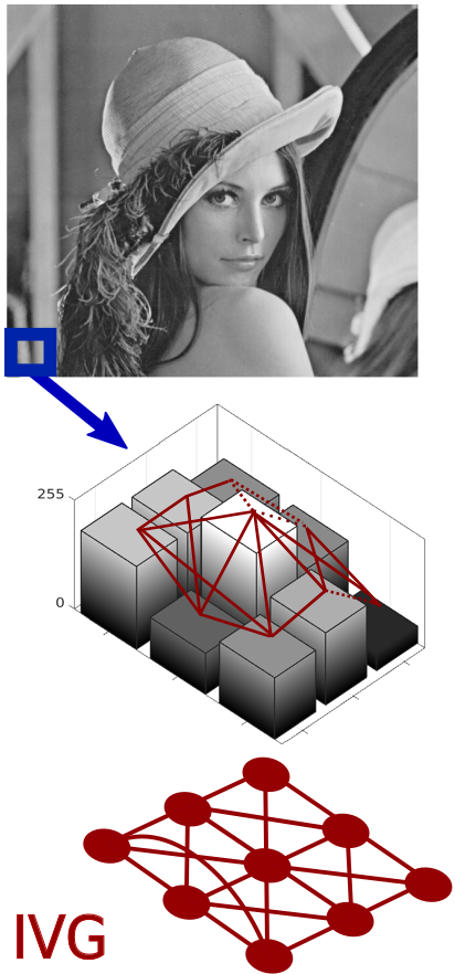
In the realm of VG/HVGs nodes have a pre-specified (temporal) ordering, and therefore these sequences inherit such order: the degree sequence is such that is the degree of the node associated to datum . These considerations can be extended to the image setting considered here, as similar labels can be attached to the nodes of an IVG/IHVG. By construction however, it is natural to order the node set of an IVG/IHVG in terms of an array (matrix) which represents the spatial positions of the associated pixels in the image. In this sense, one can therefore define the degree plot, the node clustering plot, etc, as primary topological properties of the IVG/IHVGs. For illustration, in Figure 1 we depict the process of extracting the degree plot of the IHVG associated to a grayscale image. In the degree plot (also called k-filtered image, see section III) the pixel values correspond to the degree of the nodes in the IHVG.
In section III we will use the topological plots for image filtering and compression. Before that, we need to introduce a few other features which will be relevant for image classification.
II.2 Global features: Degree distribution
Assuming the premise that the IVG/IHVG inherits information of the associated image, a natural procedure is to extract features from these graphs and use them for image classification purposes. Now, graph properties can be classified into global properties (accounting for topological information of the whole graph), or local properties (which account for properties of small substructures). Global features include the degree distribution , defined as the percentage of nodes that have degree , and other properties of the degree sequence, clustering distribution, spectral properties, distribution of cycles, etc.
In the context of visibility graphs, a recent theorem [9] proved that under suitable conditions, HVGs are in bijection with their degree sequence, suggesting that the degree distribution is indeed a relevant and informative global property. Additionally, it has been shown that can be computed exactly for simple images and is a good feature to distinguish different sorts of spatio-temporal dynamical systems [31]. Justified by these previous findings and for the sake of parsimony we will focus hereafter on as the global feature under study.
II.3 Local features: Visibility Patches
Opposed to global features, we might be interested in studying local properties of the image visibility graphs, and in this subsection we introduce a set of novel features which aims at detecting such properties. The procedure consists in counting repetitions of small subgraphs in the IVG/IHVG associated to a given image (see Figure 2 for an illustration). We call these subgraphs Visibility Patches (VPs) and we formally define them in the following way:
Definition (Visibility Patch) Consider an IVG of nodes with adjacency matrix associated to an real-valued image matrix. A Visibility Patch of order VPp is any subgraph of the IVG formed by a set of nodes for arbitrary that satisfy .
Note that the definition above extends naturally to Horizontal Visibility Patches of order p (HVPp) if the graph under study is IHVG instead of IVG.
The lowest order that yields nontrivial visibility patches is . These visibility patches can be detected by sliding a cell of size pixels with stride 1 along the entire image, and extracting the corresponding IVG/IHVGs within the cell, as shown in Figure 2. For the sake of exposition we will focus on in this work, but note that algorithms are scalable to higher orders if higher performance is needed.
A relevant quantity that summarises the abundance of visibility patches is given by the frequency distribution of each of these patches, labelled (Horizontal) Visibility Patch Profile Z (we label this profile with the bold letter Z indistinctively for patches computed on IHVG and IVG, and context will suggest which one of the two it applied to).
Interestingly, note that the concept of visibility patch is the natural extension to images of the concept of sequential visibility graph motifs [11, 36]. As a matter of fact, algorithmic computation of visibility patches reduces to checking for the presence or absence of certain combination of visibility graph motifs. This fact enables mathematical tractability of Visibility Patches as well as the design of a linear time algorithm to extract visibility patches, as we show below.
| Label | Motif | HVG | VG |
|---|---|---|---|
| 0 | |||
| 1 |
Enumeration. By construction, an (Horizontal) Visibility Patch of order , (H)VPp, is composed by an ordered sequence of sequential visibility graph motifs of order [11, 36], along the rows, columns and the main diagonal and anti-diagonal of the patch, supplemented by an additional number of motifs of lower order associated to the off-diagonals and off-anti-diagonals: 4 motifs of order , 4 motifs of order , and so on. Accordingly, a natural enumeration of a given (H)VPp is via a (2p+2+q)-dimensional vector given by
where each element of this vector enumerates the label of the actual visibility graph motif in the direction it represents. For example, in figure 3 we consider an example for the simpler nontrivial case . There are only two possible (horizontal) sequential visibility graph motifs of order 3 (see table 1) –which we can label 0 and 1– and a single possibility for motifs of order two –and therefore these do not contribute to the combinatorics–. This yields a total of different possible patches, which can be enumerated by a dimensional vector. As there are just two non-trivial motifs of order 3, one can enumerate all possible patches of order by interpreting as the binary expansion of its label, i.e.
such that for the particular case reported in Fig. 3, we find the motif label 0 in all rows, columns and diagonals except the first row, the last column and the main diagonal, i.e. , i.e. corresponding to patch no. 135.
Linear time recognition algorithm. By further capitalizing on the relation between Visibility Patches and Visibility motifs, we can build an algorithm to estimate the Visibility Patch profile Z of a given image which scales linearly with the number of pixels of the image. In particular, recognition of motifs of any order can be done in linear time by using the inequality set in Table 1 (see [11, 36] for an explicit inequality set for ). For an illustration, consider the concrete case of HVP3. We initially define for each patch, and then update the 1s in each patch according to the Algorithm 1 displayed beside, updating the HVP3 profile for each pair (computation of VP3 would follow equivalently).
In Fig. 4 we plot how runtime scales as a function of the size of the image (in number of pixels), for randomly-generated grayscale images , showcasing a linear time complexity and therefore an efficient feature extraction.
Theoretical analysis of visibility patches, including analytical results for the visibility patch profiles, is in principle possible and will be published elsewhere [37]. Here we are interested in exploring the performance of these features in practical situations. In section IV we will explore the performance of global features (e.g. degree distribution) and local features (patch profiles of order 3, as computed from (H)VP3, these being the simplest nontrivial patches) in different image classification tasks.

II.4 Multiplex features
To round off this section, we now consider the situation where one might wish to handle a set of images at once. Examples include (i) RGB images, where a given image is actually built by combining three channels (R, G and B), (ii) a given image filtered in different ways (e.g. a set of different topological plots, or image filters at different frequency bands, etc), (iii) a ‘temporal’ image comprised of a certain number of snapshots, etc. In every case, the image under study is actually a set of images (for an RGB image, ). One might then be interested in extracted the image visibility graph of each sub-image separately, or construct the image visibility graph of the image set at once. In this latter case, this naturally leads to the construction of an Image Multiplex Visibility Graph, i.e. the image version of a multiplex visibility graph [3]:
Definition (Image Multiplex Visibility Graph) Let be an ordered sequence of grayscale images. The image multiplex visibility graph is a multiplex visibility graph of layers, where layer encodes the image visibility graph of grayscale image .
Note that the resulting graph is a multiplex network, a specific type of multilayer network [6, 7] characterised by a unique set of nodes which is connected differently on several independent layers or networks (see [38] for another recent proposal for multilayer graph-based analysis of RGB images). This architecture is possible thanks to the natural alignment of every pixel in each sub-image ( aligned with ). As it is customary in multiplex networks [6, 7, 44], one can proceed to extract features from the image multiplex visibility graph of several kinds:
- 1.
- 2.
- 3.
Intrinsically multiplex descriptors: these are features that can be extracted only by considering the overall multiplex architecture of the network [50, 56], for example multiplex clustering coefficients and multiplex motifs [55, 54], node multiplex centrality measures [52, 53], and multiplex communities [51, 49].
In this work we explore the performance of efficiently combining simple intra-layer descriptors to obtain pseudo-multiplex descriptors. Indeed, a natural procedure is to take into account the whole multiplex structure and process in parallel the structural information contained in each layer by applying a method of dimensionality reduction such as Principal Component Analysis to project the concatenated feature vector of intra-layer descriptors into an adequate subspace (see Fig. 5 for an illustration). In section IV we will illustrate the use of image multiplex visibility graphs as a feature extraction method for texture classification.
III Filtering and Compression
III.1 Robustness to noise
We initially explore the robustness against noise pollution of the family of image visibility graphs. We consider the standard grayscale Lena image and pollute it with white Gaussian noise of different power. We then measure, for each level of noise to signal ratio (NSR), the similarity between the non-polluted and the polluted case. For that sake we measure the overall link overlap between the image visibility graphs extracted from the original image and the respective image visibility graph extracted from the image contaminated with noise, defined as:
| (1) |
where and denote the adjacency matrices associated to the image visibility graph from the original image and the polluted image, respectively. is the number of links that by construction two IVG/IHVGs of the same size always share because of the common lattice structure: . The overlap could be used as a general indicator of the similarity between two images of the same size or of the quality of a given image after a certain noise or filter is applied, however it doesn’t saturate to zero when comparing, say, two instances of white noise. We can build a well-defined similarity function as it follows:
| (2) |
where . By construction, this similarity measure is equal to one for equal images and reaches zero when the image is polluted with noise with a .
In Fig.6 we plot in semi-log scale (computed in both IVG and IHVG) as a function of the NSR. For comparison, we also examine the robustness against noise directly on the images by measuring a properly rescaled normalized mutual information NMI
| (3) |
Results suggest that information extracted in IVG/IHVG is more robust to noise contamination than the raw information present in the image. This result is on agreement with previous works that showcase equivalent noise robustness results in VG/HVGs [2, 11].

III.2 Visibility Filters
The results shown in Fig.6 demonstrate that IVG/IHVGs encapsulate information which is robust against noise contamination. This virtue opens the possibility of using IVG/IHVGs to handle real images, which by construction are always polluted with noise. In this subsection we consider employing the IVG/IHVGs as filters.
Definition (Visibility filter). Let be a matrix where . We define the visibility filtered image, or simply visibility filter as a matrix whose element corresponds to the value of a specific node property of the node of the associated IVG, such as its degree or its clustering coefficient. If the property is a real scalar quantity, then this quantity is opportunely rescaled to grayscale integer values. The horizontal visibility filter follows equivalently.
The above definition of a visibility filter reduces to a particular topological plot with a trivial rescaling, which allows to compare across different node properties in comparable ranges (grayscale intensity range in ).

A priori one can use many different node properties to define such filters: here we focus on three of the simplest properties, namely degree, clustering and degree-degree [4] to define three filters :
- •
-filter: when we assign to the degree of node . No rescaling is necessary here.
- •
-filter: when we assign to the local clustering coefficient (rescaled in ) of node .
- •
-filter: when we assign to the closest integer value from the average nearest-neighbors degree of node .
In Fig. 7 we plot the original grayscale Lena image () together with the three filters in a reverse grayscale. By observing these filtered images it’s easy to notice that many important details (for example details in the Lena face and in the hat) are still recognizable, but the information from the original image has been certainly compressed. Accordingly, we briefly explore compression properties of these filters in the next subsection.
III.3 Compression
In grayscale, a generic squared image has pixels and each pixel can take values, so the image size is bytes. In the IHVG -filter, each pixel corresponds now to the degree of the associated node. We know that by construction in HVGs, neglecting boundary effects, we have . Now, there is a theorem that guarantees that for white noise images, the degree distribution of decays exponentially [31], so the probability of finding a degree larger than is
To give an idea of the order of magnitude, for , this probability is lower than 0.015, i.e. less than of the nodes have a degree larger than 24. In other words, if we decided to cut-off information of the degree and assign for all nodes whose degree is larger or equal to , we would only cut-off less than of the nodes in the -filter of a white noise image. Now, at least in the 1D (time series) version it is known that the degree distribution of HVGs also decays exponentially in the typical case (not just for white noise), so we expect that a similar behaviour takes place in the image setting, and thus the probability of finding large degrees is, generically, exponentially small. This actually explains why no rescaling in practice is necessary to construct a -filter.
If no cut-off is set on the degree, there is an exponentially vanishing (although not zero) probability of finding that a node gets degree , for any . In practice, by setting a cut-off value (for instance set ) such that we assign the value to all the pixels whose actual degree is either or larger, by construction,
Note that for we only need bytes, so we have a size reduction with minimal degradation.
| FCP | FCPα=.05 | s(), s() | ||||||
|---|---|---|---|---|---|---|---|---|
| Lena | 1.24 | 1.73 | 263.2 kB | 223.9 kB | 153.8 kB | 0.85 | 0.58 | 0.69 |
| cameraman | 1.41 | 1.82 | 263.2 kB | 161.8 kB | 136.3 kB | 0.62 | 0.52 | 0.84 |
| pirate | 1.3 | 1.73 | 263.2 kB | 221.6 kB | 154.8 kB | 0.84 | 0.59 | 0.7 |
| peppers | 1.33 | 1.8 | 263.2 kB | 143.8 kB | 137 kB | 0.55 | 0.52 | 0.95 |
| house | 1.45 | 1.82 | 263.2 kB | 129.9 kB | 103 kB | 0.49 | 0.39 | 0.79 |
| mandryl | 1.33 | 1.71 | 263.2 kB | 231.9 kB | 147.8 kB | 0.88 | 0.56 | 0.63 |
| livingroom | 1.28 | 1.74 | 263.2 kB | 221 kB | 155.1 kB | 0.84 | 0.59 | 0.7 |
In order to make a systematic analysis of the different filters, we define the size of the original Lena image as
where in our case , and the size of the filtered Lena images , or simply as
where is a node-value cut-off in the filtered image. Incidentally, note that in IHVGs the minimum degree is , so the numerator in the preceding equation should read instead of , however for generality we stick with the definition above (not all filters have lower bound values) and only note that, in what follows, results for the case of the degree filter are being rather conservative.
This in turn enables us to define a general filter compression power (FCP) as the ratio
When no cut-off is enabled on to the filter, then , and the corresponding value of FCP reduces to the natural compressing power of the filter.

By lowering the value of below we can further increase the effective compression power at the expenses of deliberately degrading the filtered image. To study how much information from the original image the IVG/IHVG filters are still able to encode given any arbitrary level of compression ratio, we now need to use a measure of spatial information. To this aim we shall compute an image complexity (IC) which can be estimated using standard compressor (zip) algorithms, such that
| (4) |
where is the measured size in kB of the image given by the computer machine after saving the images in bitmap format, and is the measured size in kB of the zipped file of the image compressed using a Lempel-Ziv-type compressing algorithm. All over this work we use Matlab’s zip routine.
Accordingly, we can then quantify how much image complexity of the original image is encapsulated by different filters at any desired level of compression power. In Figure 8 (panel a) we plot the ratio as a function of FCP, for the three IHVG filters under study for a range of cut-off values (a similar analysis can be performed on IVG, data not shown). Increasing values of FCP corresponds to lowering the value of the cut-off. In Figure 8 b),c) and d) the distribution of the node-values for the different filters (degree, clustering and degree-degree) are reported to better understand the curves.
If no or very little compression is necessary, we find that the -filter (for which the clustering distribution is broad) almost encapsulates all the original image complexity ( 0.97 for FCP1) and performs better than the -filter and of the -filter. The drawback of this filter is that the information it encapsulates is rapidly degraded when one wishes to achieve even a modest level of compression ( 0.2 for FCP=1.5). On the other hand, the -filter (whose degree distribution is peaked and exponentially decaying) is able to still encapsulate high content of information even when a high level of compression is set ( 0.5 at FCP=2).
The curves also suggest that it is possible to improve consistently the -filter natural compressing power by getting rid of a very little fraction of the spatial information encoded by the filter.
According to these results, we can now define a filter optimal compressing power (FCPα) for the value of the cut-off for which
where is a parameter which measure the maximum tolerance on the amount of information degraded by the filter and has to be small.
Here we set =0.05 and we test the performance of the -filter as a compressor on several standard grayscale images (the images can be found in the Image Database website11
1
http://imageprocessingplace.com and are plotted together with their corresponding -filtered images in Fig. 9). Results are summarised in Table 2.
III.4 IHVG filters for image pre-processing
Consider a standard problem in image processing: visual face recognition. The canonical approach consists in extracting from each image a feature vector and subsequently feed classifiers with these vectors, for supervised learning.
In some cases the performance of the classifier can be improved if images are pre-processed (i.e. before feature extraction) [69]. For example local binary patterns (LPB) [67, 65, 66] that are robust to monotonic grayscale variations are widely used in face recognition problems to overcome the fact that often images are taken in different illumination conditions or with different resolutions.
Here we test the potential of the different IVG/IHVG filters defined above as pre-processing filters for the improvement of image texture analysis [69]. To simulate real-world acquisition variability we transform an image of Lena to different resolution scales by applying to the original image a Gaussian kernel with increasing values of standard deviation. As a standard feature extraction method we then make use of the gray level co-occurrence matrix (GLCM), [35, 69] a well known texture analysis technique.
For a given resolution (kernel std value) the GLCM is computed from the image and four so-called Haralick features are extracted: Contrast (measuring local variations), Correlation (measuring joint probability occurrence of pairs), Energy (sum of squared elements of the matrix) and Homogeneity (measuring the closeness of the distribution of elements in the matrix to its diagonal), see [35] for details.
All images are then mapped into points in the 4-dimensional space spanned by the appropriately normalized Haralick features (see Fig. 11). The distance (using city-block () norm, results hold similar for an Euclidean metric) between low resolution images and the original one is subsequently computed. Intuitively, the lower , the more similar a low-resolution image is from its high-resolution version in feature space, and accordingly a classifier trained with the high-resolution version would a priori find less difficulties to correctly classify low-resolution images for the filter with overall lower values of .
The procedure is repeated several times for (i) the non-filtered image, and for (ii) filtered images using all six visibility filters (-filter, filter, and filter for IVG and IHVG); and comparison with the LBP filter is reported as well for completeness. Results are shown in Fig. 10 b), where we plot in log-log as a function of the kernel standard deviation (i.e. the larger this parameter, the lower the image’s resolution). In panel a) of the same Figure, the filter effect for the different filters used in the analysis on the Lena face is shown for illustration. We find that in the case of both IVG and IHVG -filters and the IVG -filter, appears systematically below the one for the non-filtered image, suggesting that all low-resolution images will be systematically closer (in feature space) to the high-resolution version after these specific filtering pre-processing.

IV Pattern Recognition and Texture Classification
Once we have discussed the usefulness of image visibility graphs for filtering and compression purposes, we now turn and explore their applicability as efficient and universal feature-extraction methods for the task of texture detection and classification, a classical problem in computer vision [58, 57].
Despite no rigorous mathematical definition of texture is widely accepted, textures can be intuitively defined as characteristic visual patterns arising from the spatial distribution of the pixel intensity values in images [38], and therefore they are of fundamental importance in many machine vision applications such as object tracking, face recognition and automated medical diagnosis [60].
Following recent efforts in the direction of cataloguing textures and texture-related datasets [59, 60], we will test the performance of image visibility related descriptors on different types of textures, namely textures of materials, bio-medical textures and natural textures.

| Complex Tree | Linear Discriminant | linear SVM | quadratic SVM | weighted KNN | Ensemble Bagged Tree | |
|---|---|---|---|---|---|---|
| IHVG P(k) | 100% | 96.7% | 100% | 100% | 98.8% | 100% |
| IHVG P(k)+PCA (5 PCs) | 100% | 96.7% | 100% | 100% | 100% | 99.2% |
| IVG P(k) | 95.3% | 95.8% | 99.2% | 100% | 94.2% | 98.8% |
| IVG P(k)+PCA (5 PCs) | 96.7% | 97% | 97.9% | 100% | 100% | 98.8% |
IV.1 Global features for Materials Texture Recognition
We start by showing that the degree distribution extracted from IHVGs is an ideal global feature vector for the automatic recognition of material textures. These are a specific class of textures derived by imaging the surface of various types of materials for the purpose of classifying them according to the characteristic structural patterns captured in this way. The dataset we used is a reduced version of the Kylberg Texture Dataset [39], formed by grayscale texture images from 6 different materials (canvas surface, cushion surface, line seeds, sand, seat surface and stone surface) with 40 samples per class. This dataset is often used as a benchmark for testing material texture descriptors because of the image homogeneity in terms of perspective, scale, and illumination across the different classes [40, 41]. Because of the grayscale nature of the images and the uniform texture of the materials, this is ideal to test the capability of IVG/IHVGs global features to capture the surface structural correlations and patterns. In Figure 12 a) we provide an illustration of the texture classes. Each image in the dataset is transformed to the corresponding IHVG and its degree distribution is extracted and then given in input (as a vector of features) to different classifiers. Principal component analysis (PCA) is applied to the input vectors to reduce the number of features and to avoid eventual overfitting, and a fold cross validation procedure is adopted. A (average by class) classification accuracy –defined as the percentage of samples correctly assigned to their true class– can be obtained by mean of a linear/quadratic-kernel Multiclass one-vs-one Support Vector Machine (ovo-lSVM/qSVM), for IHVG and with a quadratic-kernel SVM for IVG. Interestingly, this level of accuracy is already obtained only using the first 5 principal components of the PCA projection. To further understand why the degree distribution is such an informative feature, in Fig. 13 we plot the degree distribution for all the samples (colored by class as a guide for the eye) for the IHVGs (a) and for the IVGs (b). Distributions cluster by class and already by visual inspection we can determine the clusters. For completeness, in Table 3 we report the classification accuracies reached by different standard classifiers implemented in the Matlab Classification Learner App. For IHVGs it is possible to obtain an accuracy of by using a Complex Tree classifier or a Bagged Tree and with a weighted KNN algorithm as well after applying PCA.

IV.2 Combining Global and Local Features for Bio-medical Texture Classification
In a second step, we now focus on a more complex image dataset called 2D HeLa. This is a bio-medical dataset of grayscale fluorescence microscopy images of HeLa cells stained
with various organelle-specific fluorescent dyes able to reveal characteristic structural patterns of proteins so that 10 classes can be identified: Actin, DNA, Endosome, ER, cis-Golgi, Golgi, Lysosome, Microtubules, Mitochondria and Nucleoli. For each of these classes there is a different number of sample images (between 73 and 98), for a total of 862 images. In Fig. 12 (b) we illustrate one representative sample for each class.This dataset is exemplar with respect to the bio-medical challenge of the automated interpretation of sub-cellular protein patterns in fluorescence microscope images, which can help characterize many genes whose function is still unknown.
Unlike material textures, these images show several complex biological structures that occupy only a certain subregion of the image. This fact precludes using only global features, justifying the necessity to complement these with local features to attain high classification accuracies. Accordingly, we test the performance of the Visibility Patches.
Again, we feed the feature vector with global descriptors given by the first entries of the degree distribution of IHVGs (up to ), the degree distribution of IVGs (up to ), and a concatenation of both. Additionally, we add local features given by the visibility patch profiles of HVP3 (188 patches detected) and VP3 (249 patches detected), and a concatenation of the two. To avoid overfitting, PCA is applied to reduce the number of features before classification. The PCA-transformed features are then given in input again to a linear-kernel Multiclass one-vs-one Support Vector Machine.
The best classification accuracy is obtained by using a combination of global and local features from the blend of IHVG and IVG descriptors, reaching 83.5%.
In Table 4 we report, for each set of descriptors, the values of the best average classification accuracy and corresponding average (over the classes) area under the ROC curve (AUC) obtained over 30 realizations of the classifier, together with the average classification accuracy over of the model realizations (Model Average Accuracy MAA). In Fig. 14 we depict the details of the confusion matrix and of the ROC curves by class for the best model trained. The highest off-diagonal values in the confusion matrix correspond to pairs of classes that are expected to be hard to distinguish, for example ER and mitochondrial proteins and Golgi and cis-Golgi proteins.
The optimal number of PCs for each feature set (local/global, IVG/IHVG) is found with an exhaustive search in the space of the principal components number by measuring the average classification accuracy of the model (MAA) over 30 model realizations (see Figure 15 (a) and Table 4). The values of MAA for each descriptor tend to quickly saturate by increasing the number of components, meaning that the final model is robust with respect to the choice of the set of ).
Interestingly, we observe that while global features from the IHVG are more informative than for the IVG, the opposite is true for local features, as these seem to be more informative for IVG than for IHVG. For comparison, in the original paper [42] of the 2D HeLa dataset the authors obtained an average class accuracy of 84% by training a Back-Propagation Neural Network with specifically designed (ad-hoc) features. In other words, our parsimonious approach, using a set of non-specific graph-based features is competitive with respect to ad-hoc, context-dependent features. The highest published performance we are aware of is 95.3% [43], obtained with a multi-resolution feature extraction approach combined with a neural network classifier, and it is an open problem whether one could reach competitive results by complementing the non-specific approach designed here with problem-specific strategies.


| ovo-lSVM models | Accuracy | MAA | |||
|
75.4% | 0.939 | 74.5% | ||
|
79.5% | 0.961 | 78.6% | ||
|
83.5% | 0.973 | 83% | ||
| 2D Hela descriptors | MAA | ||||
| P(k) IVG | 14 | 57.2% | |||
| P(k) IHVG | 8 | 67.6% | |||
| IVG | 22 | 75.8% | |||
| IHVG | 23 | 74% |
IV.3 Image Visibility Multiplex for RGB Images: Natural Textures
In natural scenes, more complicated textures can arise, e.g. patterns of waves on the surface of a lake or conformation and disposition of leaves from a plant when pictured from above. These kind of textures are generally classified as natural textures and are very relevant because they can be seen as the building blocks of more complex features arising in real world scenes.
Accordingly, in this subsection we consider three well known collections of natural textures: the Upstex dataset [61], the Colored Brodatz dataset [63], and the Multiband (MTB) dataset [63]. The Upstex dataset includes 191 classes of 12 samples each showing textures from outdoor scenes such as walls, pavements, vegetation, soil, plant leaves, rocks (in Figure 12 c) we show some samples from different classes).
The Brodatz dataset in turn is among the most widely used datasets in the literature of texture analysis and comprehend scanned images from an album. In the colored version [63] of the dataset there are 112 images of size , defining a total of 112 different classes (in Figure 12 c) we report some examples). For each class there are 16 samples defined as the non-overlapping subimages of size .
Finally, the Multiband dataset is derived from the Brodatz dataset by aggregating triplets of original grayscale images in various combinations such that the resulting RGB images display a mixture of channel-dependent textures (see some examples in Figure 12 c)), totalling 154 classes and 16 samples per class.
All these three datasets are characterised by containing RGB images, many different classes, and a relatively small number of samples per class. Our approach here is to extract from each image the multiplex IVG/IHVG (by extracting the single-layer IVGs/IHVGs form each of the image channels: R,G,B) and obtain pseudo-multiplex descriptors by blending global/local features of each channel via PCA (see Figure 5).
To obtain the highest classification performance we extracted global and local pseudo-multiplex features from both the multiplex IHVG and the multiplex IVG and we used a quadratic-kernel Multiclass one-vs-all Support Vector Machine (ova-qSVM), 10-fold cross validation.
In order to optimize the number of components for each of the multiplex local/global features we follow a methodology analogous to the one used for the 2DHela dataset, but this time, to prove the efficiency of our classifier we tuned the number of principal components of the features only once for all the datasets by optimising the average classification accuracy of the model (MMA) over 30 model realizations measured on the sub-set of data of the Usptex dataset which includes only the first 50 classes (Figure 15 (b)).
In Table 5 we report for each of the datasets the values of accuracy, average AUC per class and MAA obtained with the model trained with global, local and global+local multiplex features.
Our best classification accuracy for Usptex, Brodatz and Multiband is respectively , , and is obtained with only 53 features that are a combination of multiplex local and global features from IHVG and IVG. Interestingly, in a very recent paper [38] the authors evaluated the performance of several pre-trained state-of-the-art convolutional neural network to two of these dataset (Usptex and Multiband), blended together with the performance obtained by extracting features from a so-called Multilayer Complex Network (Multilayer CN) in a similar spirit with respect to our multiplex approach. They report that as the best accuracy ever published for Usptex, that they obtain with a pre-trained ResNet50 2016, and the best accuracy for Multiband obtained with their Multilayer Complex Network classifier. To the best of our knowledge we obtained the highest performance ever on the Multiband dataset, which suggests that our multiplex approach is ideal for detecting multi-band texture features and outperforms traditional CNN feedforward architectures, including the Multilayer CN proposed in [38], that perhaps drop in performance because they are designed to learn texture features both from intra-band and inter-band pixel correlations.
Regarding the Brodatz colored dataset, we couldn’t find any reference value of performance reported in literature, however for the grayscale original dataset a classification accuracy of was recently obtained via an hybrid classifier which combines a Convolutional Neural Network and a Support Vector Machine [64].
| ova-qSVM | Accuracy | MAA | |||||||||||||||
|---|---|---|---|---|---|---|---|---|---|---|---|---|---|---|---|---|---|
|
|
|
| ||||||||||||||
|
|
|
| ||||||||||||||
|
|
|
|
V Conclusion
The family of image visibility graphs IVG/IHVGs extract graphs from images and extend the concept of visibility graph time series analysis to image processing. In this paper we have showcased that this mapping can be leveraged to make (i) image filtering, (ii) compression and (iii) classification by extracting simple, universal (non-specific) and computationally efficient (i.e. fast and scalable extraction) features.
In a first step, we have shown how these graphs can be used to define filters for image preprocessing and image compression, which show good performance and are based on a methodology which is conceptually different from standard time/frequency domain filtering techniques.
Furthermore, by defining both global features (e.g. degree distribution) and local features (e.g. visibility patches, a novel tool which extends the concept of sequential visibility graph motifs [11, 36] to images) we are able to reach competitive results in image classification tasks, sometimes superior to state of the art results obtained by sophisticated algorithms with highly specialised context-dependent descriptors. We found that global features seem to be more informative when extracted from the IHVG than from IVG, while the opposite is true for local features (e.g. patches), at least for low-order patches (). We shall highlight that results are performed using low-order visibility patches (), so better performance is likely to be obtained with higher order (e.g. ), for which linear time algorithms can also be designed [11, 36]. An hybrid combination of our newly defined set of visibility graph features with more standard ad-hoc (i.e. problem-dependent) features and automatic feature extraction methods (e.g. artificial neural networks) is likely to provide even better results: this is an open problem for further research.
We should emphasize that the set of features extracted from IVG/IHVG –such as degree distributions or visibility patches– is universal, in the sense that they are not designed to exploit particular, context-dependent properties of the image and can therefore be measured across classification tasks of different nature. Quoting Nanni [68], “The present trend in machine learning is focused on building optimal classification systems for very specific, well-defined problems. Another research focus, however, would be to work on building General-Purpose (GP) systems that are capable of handling a broader range of problems as well as multiple data types. Ideally, GP systems would work well out of the box, requiring little to no parameter tuning but would still perform competitively against less flexible systems that have been optimized for very specific problems and datasets.”
Accordingly, we envisage that this methodology can have a potential impact in pattern recognition and image classification tasks across the disciplines, opening a plethora of further research directions. From a theoretical perspective, we recall that visibility graphs designed for time series analysis purposes have been shown previously to be amenable to analytic insight [10]. We conjecture that theoretical analysis –including analytical results– for image visibility graphs is also possible.
Other interesting open problems for further research include: (i) capitalizing on the properties of multiplex networks for extracting correlation-based multiplex features from RGB images, such as degree-degree correlations across layers [44], and the (ii) use the multiplex setting to study under a single framework videos (ordered sequence of images).
Acknowledgments. Thanks to N. Sadawi for interesting discussions. LL acknowledges funding from EPSRC Fellowship EP/P01660X/1. JI acknowledges funding from Wellcome Trust Metaboflow Grant 202952Glen.
References
- [1] L. Lacasa, B. Luque, F.J. Ballesteros, J. Luque, and J.C. Nuno, From time series to complex networks: the visibility graph, Proc. Natl. Acad. Sci. USA 105, 13 (2008).
- [2] B. Luque, L. Lacasa, J. Luque, F.J. Ballesteros, Horizontal visibility graphs: exact results for random time series, Phys. Rev. E 80, 046103 (2009).
- [3] L. Lacasa, V. Nicosia, V. Latora, Network Structure of Multivariate Time Series, Sci. Rep. 5, 15508 (2015)
- [4] V. Latora, V. Nicosia and G. Russo, Complex Networks: Principles, Methods and Applications (Cambridge University Press, 2017)
- [5] Z-K Gao, M. Small and J. Kurths, Complex network analysis of time series, EPL 116, 5 (2017).
- [6] M. Kivela, A. Arenas, M. Barthelemy, J.P. Gleeson, Y. Moreno and M.A. Porter, Multilayer networks. J. Complex Networks 2 (3), 203-271 (2014).
- [7] S. Boccaletti, G. Bianconi, R. Criado, C.I. del Genio, J. Gomez-Gardenes, M. Romance, I. Sendina-Nadal, Z. Wang, and M. Zanin. The structure and dynamics of multilayer networks. Phys. Rep. 544 (1), 1-122 (2014).
- [8] S. Severini, G. Gutin, T. Mansour, A characterization of horizontal visibility graphs and combinatorics on words, Physica A 390, 12 (2011) 2421-2428.
- [9] B. Luque, L. Lacasa, Canonical horizontal visibility graphs are uniquely determined by their degree sequence, Eur. Phys. J. Sp. Top. 226, 383 (2017).
- [10] L. Lacasa, On the degree distribution of horizontal visibility graphs associated to Markov processes and dynamical systems: diagrammatic and variational approaches, Nonlinearity 27, 2063-2093 (2014).
- [11] J. Iacovacci and L. Lacasa, Sequential visibility-graph motifs, Phys. Rev. E 93, 042309 (2016)
- [12] L. Lacasa, B. Luque, J. Luque and J.C. Nuño, The Visibility Graph: a new method for estimating the Hurst exponent of fractional Brownian motion, EPL 86 (2009) 30001.
- [13] B. Luque, L. Lacasa, F. Ballesteros, A. Robledo, Analytical properties of horizontal visibility graphs in the Feigenbaum scenario, Chaos 22, 1 (2012) 013109.
- [14] B. Luque, A. Núñez, F. Ballesteros, A. Robledo, Quasiperiodic Graphs: Structural Design, Scaling and Entropic Properties, Journal of Nonlinear Science 23, 2, (2012) 335-342.
- [15] A.M. Núñez, B. Luque, L. Lacasa, J.P. Gómez, A. Robledo, Horizontal Visibility graphs generated by type-I intermittency, Phys. Rev. E, 87 (2013) 052801.
- [16] Shao, Z. G. Network analysis of human heartbeat dynamics. Applied Physics Letters, 96, 7 (2010) 073703.
- [17] Ahmadlou M, Adeli H, Adeli A. New diagnostic EEG markers of the Alzheimer’s disease using visibility graph. Journal of neural transmission 117(9) (2010)1099-109.
- [18] Ahmadlou, M., Adeli, H., & Adeli, A. Improved visibility graph fractality with application for the diagnosis of autism spectrum disorder. Physica A 391, 20 (2012) 4720-4726.
- [19] Bhaduri, S., & Ghosh, D. Electroencephalographic data analysis with visibility graph technique for quantitative assessment of brain dysfunction. Clinical EEG and neuroscience 46, 3 (2015), 218-223.
- [20] Sannino, S., Stramaglia, S., Lacasa, L., & Marinazzo, D. Visibility graphs for fMRI data: multiplex temporal graphs and their modulations across resting state networks. Network Neuroscience (2017)
- [21] S. Jiang, C. Bian, X. Ning and Q.D.Y. Ma, Visibility graph analysis on heartbeat dynamics of meditation training, Appl. Phys. Lett. 102 253702 (2013).
- [22] U. Hasson, J. Iacovacci, B. Davis, R. Flanagan, E. Tagliazucchi, H. Laufs, L. Lacasa A combinatorial framework for peak/pit asymmetry in complex dynamics, Sci. Rep. 8, 3557 (2018).
- [23] A. Aragoneses, L. Carpi, N. Tarasov, D.V. Churkin, M.C. Torrent, C. Masoller, and S.K. Turitsyn, Unveiling Temporal Correlations Characteristic of a Phase Transition in the Output Intensity of a Fiber Laser, Phys. Rev. Lett. 116, 033902 (2016).
- [24] M. Murugesana and R.I. Sujitha1, Combustion noise is scale-free: transition from scale-free to order at the onset of thermoacoustic instability, J. Fluid Mech. 772 (2015).
- [25] A. Charakopoulos, T.E. Karakasidis, P.N. Papanicolaou and A. Liakopoulos, The application of complex network time series analysis in turbulent heated jets, Chaos 24, 024408 (2014).
- [26] P. Manshour, M.R. Rahimi Tabar and J. Peinche, Fully developed turbulence in the view of horizontal visibility graphs, J. Stat. Mech. (2015) P08031.
- [27] RV Donner, JF Donges, Visibility graph analysis of geophysical time series: Potentials and possible pitfalls, Acta Geophysica 60, 3 (2012).
- [28] V. Suyal, A. Prasad, H.P. Singh, Visibility-Graph Analysis of the Solar Wind Velocity, Solar Physics 289, 379-389 (2014)
- [29] Y. Zou, R.V. Donner, N. Marwan, M. Small, and J. Kurths, Long-term changes in the north-south asymmetry of solar activity: a nonlinear dynamics characterization using visibility graphs, Nonlin. Processes Geophys. 21, 1113-1126 (2014).
- [30] J.F. Donges, R.V. Donner and J. Kurths, Testing time series irreversibility using complex network methods, EPL 102, 10004 (2013).
- [31] L. Lacasa, J. Iacovacci, Visibility graphs of random scalar fields and spatial data Phys. Rev. E 96, 012318 (2017)
- [32] A. Turner, M. Doxa, D. O’sullivan, and A. Penn, From isovists to visibility graphs: a methodology for the analysis of architectural space. Environment and Planning B: Planning and design 28 (1), 103-121 (2001).
- [33] Lézoray, O. and Grady, L. eds., 2012. Image processing and analysis with graphs: theory and practice. CRC Press.
- [34] R. Gonzalez, Rafael, Digital Image Processing, 3rd (Pearson Hall, 2008).
- [35] Haralick, R.M. and Shanmugam, K., 1973. Textural features for image classification. IEEE Transactions on systems, man, and cybernetics, (6), pp.610-621.
- [36] J. Iacovacci and L. Lacasa, Sequential motif profile of natural visibility graphs Phys. Rev. E 94, 052309 (2016).
- [37] L. Lacasa, J. Iacovacci, Theory of visibility patches, in preparation.
- [38] L.F.S. Scabini, R.H.M. Condori, W.N. Gonçalves, O.M.Bruno, Multilayer Complex Network Descriptors for Color-Texture Characterization, arXiv:1804.00501v1
- [39] G. Kylberg. The Kylberg Texture Dataset v. 1.0, Centre for Image Analysis, Swedish University of Agricultural Sciences and Uppsala University, External report (Blue series) No. 35. Available online at: http://www.cb.uu.se/?gustaf/texture/
- [40] Kylberg G., and Sintorn I.-M. Evaluation of Noise Robustness for Local Binary Pattern Descriptors in Texture Classification EURASIP Journal on Image and Video Processing, 2013, 17.
- [41] Andrearczyk, V. and Whelan, P.F., 2016. Using filter banks in convolutional neural networks for texture classification. Pattern Recognition Letters, 84, pp.63-69.
- [42] Boland, M.V. and Murphy, R.F., 2001. A neural network classifier capable of recognizing the patterns of all major subcellular structures in fluorescence microscope images of HeLa cells. Bioinformatics, 17(12), pp.1213-1223.
- [43] A. Chebira, Y. Barbotin, C. Jackson, T. Merryman, G. Srinivasa, R.F. Murphy, and J. Kovacevic (2007). A multiresolution approach to automated classification of protein subcellular location images. BMC Bioinformatics 8:210.
- [44] F. Battiston, V. Nicosia, and V. Latora, Structural measures for multiplex networks, Phys. Rev. E 89, 032804 (2014).
- [45] Boccaletti S, Bianconi G, Criado R, Del Genio CI, Gómez-Gardenes J, Romance M, et al. The structure and dynamics of multilayer networks. Physics Reports 544(1):1–122 (2014).
- [46] Bianconi G. Statistical mechanics of multiplex networks: Entropy and overlap. Physical Review E. 87(6):062806 (2013)
- [47] Nicosia V, Latora V. Measuring and modeling correlations in multiplex networks. Physical Review E. 92(3):032805 (2015)
- [48] Iacovacci J, Wu Z, Bianconi G. Mesoscopic structures reveal the network between the layers of multiplex data sets. Physical Review E 92(4) 042806 (2015)
- [49] De Domenico M, Lancichinetti A, Arenas A, Rosvall M. Identifying modular flows on multilayer networks reveals highly overlapping organization in interconnected systems. Physical Review X. 2015;5(1):011027.
- [50] Iacovacci, J. and Bianconi, G., 2016. Extracting information from multiplex networks. Chaos: An Interdisciplinary Journal of Nonlinear Science, 26(6), p.065306.
- [51] Mondragon, R.J., Iacovacci, J. and Bianconi, G., 2018. Multilink communities of multiplex networks. PloS one, 13(3), p.e0193821.
- [52] Iacovacci, J., Rahmede, C., Arenas, A. and Bianconi, G., 2016. Functional multiplex pagerank. EPL (Europhysics Letters), 116(2), p.28004.
- [53] Halu, A., Mondragón, R.J., Panzarasa, P. and Bianconi, G., 2013. Multiplex pagerank. PloS one, 8(10), p.e78293.
- [54] Cozzo, E., Kivelä, M., De Domenico, M., Solé-Ribalta, A., Arenas, A., Gómez, S., Porter, M.A. and Moreno, Y., 2015. Structure of triadic relations in multiplex networks. New Journal of Physics, 17(7), p.073029.
- [55] Battiston, F., Nicosia, V., Chavez, M. and Latora, V., 2017. Multilayer motif analysis of brain networks. Chaos: An Interdisciplinary Journal of Nonlinear Science, 27(4), p.047404.
- [56] Cardillo A, Gómez-Gardenes J, Zanin M, Romance M, Papo D, Del Pozo F, et al. Emergence of network features from multiplexity. Scientific reports. 2013;3:1344.
- [57] Sonka, M., Hlavac, V. and Boyle, R., 2014. Image processing, analysis, and machine vision. Cengage Learning.
- [58] Liu, L., Chen, J., Fieguth, P., Zhao, G., Chellappa, R. and Pietikainen, M., 2018. A Survey of Recent Advances in Texture Representation. arXiv preprint arXiv:1801.10324.
- [59] Hossain, S. and Serikawa, S., 2013. Texture databases: a comprehensive survey. Pattern Recognition Letters 34(15), pp.2007-2022.
- [60] Bianconi, F. and Fernández, A., 2014. An appendix to Texture databases: A comprehensive survey. Pattern recognition letters, 45, pp.33-38.
- [61] Backes, A.R., Casanova, D. and Bruno, O.M., 2012. Color texture analysis based on fractal descriptors. Pattern Recognition, 45(5), pp.1984-1992.
- [62] Brodatz, P., 1966. A Photographic Album for Arts and Design.
- [63] Abdelmounaime, S. and Dong-Chen, H., 2013. New Brodatz-based image databases for grayscale color and multiband texture analysis. ISRN Machine Vision 2013.
- [64] Adly, H. and Moustafa, M., 2017. A hybrid deep learning approach for texture analysis. arXiv preprint arXiv:1703.08366.
- [65] Nanni, L., Lumini, A. and Brahnam, S. Survey on LBP based texture descriptors for image classification. Expert Systems with Applications 39, 3 (2012) pp.3634-3641.
- [66] Jain, L.C., Nanni, L. and Lumini, A, eds. Local binary patterns: new variants and applications (Springer, 2016)
- [67] Ojala, T., Pietikäinen, M. and Harwood, D., 1996. A comparative study of texture measures with classification based on featured distributions. Pattern recognition, 29(1), pp.51-59.
- [68] Nanni, L., Brahnam, S., Ghidoni, S. and Lumini, A., 2015. Toward a general-purpose heterogeneous ensemble for pattern classification. Computational intelligence and neuroscience, 2015, p.85.
- [69] Nanni, L., Brahnam, S., Ghidoni, S. and Menegatti, E., 2015. Improving the descriptors extracted from the co-occurrence matrix using preprocessing approaches. Expert Systems with Applications, 42(22), pp.8989-9000.