Entropy rates for Horton self-similar trees

In this paper, a $\mathit{tree}$ is defined as an acyclic connected graph. A tree with one vertex labeled as the $\mathit{root}$ is called a $\mathit{rooted}$ $\mathit{tree}$. Presence of the root in a tree provides a natural child-parent relation between the neighboring vertices. More precisely, the $\mathit{parent}$ of a vertex is the vertex connected to it on the path down, towards the root and the $\mathit{child}$ of a vertex is the vertex connected to it on the path up, away from the root. Note that a vertex can have more than one child and every vertex except the root has a unique parent and a unique $\mathit{parental}$ $\mathit{edge}$ that connects a vertex to its parent. A $\mathit{leaf}$ is a vertex with no children. The $\mathit{degree}$ of a vertex is the number of edges incident to a vertex.

A tree is called a $\mathit{binary}$ tree if each vertex has at most two children. A $\mathit{full}$ binary tree is a tree in which every vertex has either zero or two children. A $\mathit{perfect}$ binary tree is a binary tree in which all interior vertices have two children and all leaves have the same depth. In Figure 1 (a) and (b) we depict full and perfect binary trees, respectively. A $\mathit{plane}$ tree is a rooted tree with a specified ordering for the children of each vertex. This ordering is equivalent to an embedding of the tree in the plane and provides a natural left and right orientations for the children. A $\mathit{planted}$ $\mathit{binary}$ $\mathit{plane}$ $\mathit{tree}$ is a rooted tree such that its root has degree one and every other vertex is either a leaf or an $\mathit{internal}$ $\mathit{vertex}$ of degree three (see section 7.2 in [25]). We denote a $\mathit{stem}$ to be the unique edge that connects the root vertex with its only child. Assuming the tree grows from the root vertex upwards, the root vertex is located at the bottom of the stem. Every planted binary plane tree with $n$ leaves has $2n-1$ edges and even number of vertices $2n$, such that $n-1$ of them are internal. For examples, see Figure 1 (c) and (d).

In this paper, we consider the space of finite unlabeled rooted binary plane trees with no edge length. We denote this space by $\mathcal{T}$. Let $\mathscr{T}_{N}\subset\mathcal{T}$ be the space of all planted binary plane trees with $n$ leaves and $N=2n$ vertices. The number of possible configurations of a planted binary plane tree with $N$ vertices is given by the $(n-1)$th Catalan number $\mathcal{C}_{n-1}$ [25] as follows

where $n=\frac{N}{2}$ and ${n\choose k}=\frac{n!}{k!(n-k)!}.$

The Horton-Strahler ordering of the vertices and branches in a binary tree is performed, from the leaves to the root node, by hierarchical counting [16, 11, 7, 8, 13, 26] as follows

• •

  each leaf is assigned order $1$;

• •

  an internal vertex with children of orders $i$ and $j$ is assigned the order $k=\max(i,j)+\delta_{ij},$ where $\delta_{ij}$ is the Kronecker’s delta;

• •

  the parental edge of the vertex has the same order as the vertex;

• •

  a $\mathit{branch}$ of order $i$ is a sequence of neighboring vertices of order $i$ together with their corresponding parental edges.

The order $K$ of a non-empty tree is defined as the maximal order of its vertices. The $\mathit{Horton-Strahler}$ $\mathit{ordering}$ of a tree is defined as a set of numbers $N_{i}$, $i=\overline{1,K}$, where $N_{i}$ is the number of branches of order $i$. Note that

1. 1.

   in order to have a branch of order $i+1$ we need to have at least two branches of order $i$, i.e., $N_{i}\geq 2N_{i+1}$, $\forall i=\overline{1,K-1}$;

2. 2.

   a planted binary plane tree of order $K$ will have only one branch of order $K$, i.e., $N_{K}=1$.

In this work, we consider only admissible sequences, defined as the sequences $N_{1},N_{2},\cdots,N_{K}$ that satisfy the two conditions described above. We call an admissible sequence $N_{1},N_{2},\cdots,N_{K}$ a set of Horton-Strahler numbers. To illustrate the Horton-Strahler ordering of a planted binary plane tree consider an example in Figure 2.

Denote $\mathscr{T}_{N_{1}\cdots N_{K}}\subset\mathcal{T}$ be the space of all planted binary plane trees with Horton-Strahler numbers $N_{1},N_{2},\cdots,N_{K}$. Note that $\mathscr{T}_{N_{1}\cdots N_{K}}\subset\mathscr{T}_{N}$, where $N=2N_{1}$. In the next section, we present our first statement that gives $|\mathscr{T}_{N_{1}\cdots N_{K}}|$ - the number of possible planted binary plane trees with Horton-Strahler numbers $N_{1},N_{2},\cdots,N_{K}$.

Recall that entropy is a measure of the average uncertainty in the random variable [28, 29]. For a discrete random variable $X$ with possible values $x_{1},x_{2},\cdots,x_{n}$ and probability mass function $P(X)$ the entropy of $X$ is defined by

where the quantity $0\log_{2}0$ is taken to be $0$. The entropy is measured in bits. We can think of $\log_{2}P(x_{i})$ as the uncertainty of the outcome $x_{i}$ (or the “surprise” of observing $x_{i}$). Thus, the entropy is the average “surprise”. If possible values of $X$ are uniformly distributed, i.e., $P(x_{i})=1/n$, then there is a maximal uncertainty about the outcome, maximum “surprise”. In this case, the entropy achieves its maximal value $H(X)=\log_{2}n$. For example, the entropy of a fair coin toss is 1 bit. On the other hand, the occurrence of a certain event ($P(x_{i})=1$, i.e., no “surprise”) has minimal uncertainty, which corresponds to the minimal value of entropy $H(X)=0$.

From the information theory point of view, the entropy of a random variable can be thought of as an average number of bits required to describe the random variable [28]. Consider a random variable $X$ that has a uniform distribution over $8$ outcomes, e.g., an eight-sided dice. The entropy of $X$ is $H(X)=-\sum_{i=1}^{8}\frac{1}{8}\log_{2}\frac{1}{8}=\log_{2}8=3$ bits. A $3$-bit string takes on $8$ different values and is sufficient to describe $8$ outcomes of $X$. Note that all outcomes of $X$ have representations of the same $3$-bit length. Consider now a random variable $Y$ with a nonuniform distribution. Assume $Y$ can take $5$ possible values $\{y_{1},y_{2},y_{3},y_{4},y_{5}\}$ with corresponding probabilities $\left(\frac{1}{2},\frac{1}{8},\frac{1}{8},\frac{1}{8},\frac{1}{8}\right)$. The entropy of $Y$ is $H(Y)=-\frac{1}{2}\log_{2}\frac{1}{2}-4\frac{1}{8}\log_{2}\frac{1}{8}=2$ bits. Using Huffman coding technique we can encode outcome $y_{1},y_{2},y_{3},y_{4},y_{5}$ as strings $1,011,010,001,000$, respectively. Since we use shorter description for the more probable outcome $y_{1}$ and longer descriptions for the less probable outcomes $y_{2},y_{3},y_{4},y_{5}$, the average description length is equal to the value of the entropy and is exactly $2$ bits.

Consider now a space $\mathscr{T}_{N}$, and let $P$ be a probability measure over $\mathscr{T}_{N}$. We define the entropy of a random planted binary plane tree $T_{N}\in\mathscr{T}_{N}$ as follows

and consider it to be the measure of the structural complexity of a tree. Informally, the larger the entropy, the more complex is the tree’s dendritic structure. The entropy of a tree gives the average number of bits needed to encode it. In order to analyze the entropy’s growth rate as $N\rightarrow\infty$, we define the entropy rate $\mathscr{H}_{\infty}$ to be the limit of normalized entropies $H(T_{N})/N$, $T_{N}\in\mathscr{T}_{N}$ as $N\rightarrow\infty$

provided that the limit exists. The entropy rate quantifies per vertex entropy. In other words, for large $N$ the entropy rate gives the average number of bits per vertex required to encode the tree. In fact, for large $N$ there exist an arithmetic coding scheme that encodes a tree with $N$ vertices using about $N\mathscr{H}_{\infty}$ bits [30]. Arithmetic coding can get arbitrarily close to the entropy, because it does not convert each vertex separately, but assigns one codeword to the entire tree. The tree can be recreated from this codeword.

The next lemma provides a formula for the entropy of a random planted binary plane tree with $N$ vertices.

The proof of this result is given in Section VI-C.

The proof of the Corollary 1 is given in Section VI-D. Lemma 2 and Corollary 1 demonstrate that for large enough $N$, we need about $N$ bits per tree or about one bit per vertex to encode any tree $T_{N}\in\mathscr{T}_{N}$. While presented in a different context, Corollary 1 reaffirms the entropy rate of the maximum entropy model in [30].

In Section II-B we introduced a space $\mathscr{T}_{N_{1}\cdots N_{K}}$ of planted binary plane trees with an arbitrary (but admissible) set Horton-Strahler numbers $N_{1},N_{2},\cdots,N_{K}$. Quite often, however, observed tree-like structures display geometric decrease of the numbers $N_{i}$ of elements of Horton-Strahler order $i\geq 1$. This property is known as Horton self-similarity, also referred to as the Horton Law. Formally, the Horton Law states the existence of the limit $\lim_{i\rightarrow\infty}N_{i}/N_{i+1}=R$, where the quantity $R$ is called the Horton exponent. There are multiple models with broad range of Horton exponents that appear in different scientific areas and have practical importance in a variety of applications [16, 13, 11, 31, 19]. For example, a perfect binary tree satisfies the Horton law with $R=2$ while the critical binary Galton-Watson tree [16, 11, 25, 32] satisfies the Horton law with $R=4$. The real river networks have Horton exponent $R$ in a range $(3,5)$ [33, 7], e.g., for Amazon river $R=4.51$ and for Mississippi river $R=4.69$. In fact, for many natural tree-like structures $R\in(3,5)$. It was confirmed in hydrology [27, 34, 11, 35, 36, 37], biology, and other areas [13].

Next, we introduce a space of planted binary plane trees that satisfy Horton law with Horton exponent $R$ and examine its entropy rate.

Let $\mathscr{T}_{K,R}$ be a space of planted binary trees with $N$ vertices and the Horton-Strahler numbers $N_{k}$, $\forall k=\overline{1,K}$ that are defined in a special form as follows

where $R,\alpha\in\mathbb{R}$ such that $R>2$ and $\alpha\in(1,R)$. In other words, $N_{k}\approx R^{K-k}$ with an error $N_{k}-R^{K-k}$ dominated by the power of an exponent smaller than $R$. It is easy to see that this model satisfies the Horton law with Horton exponent $R$.

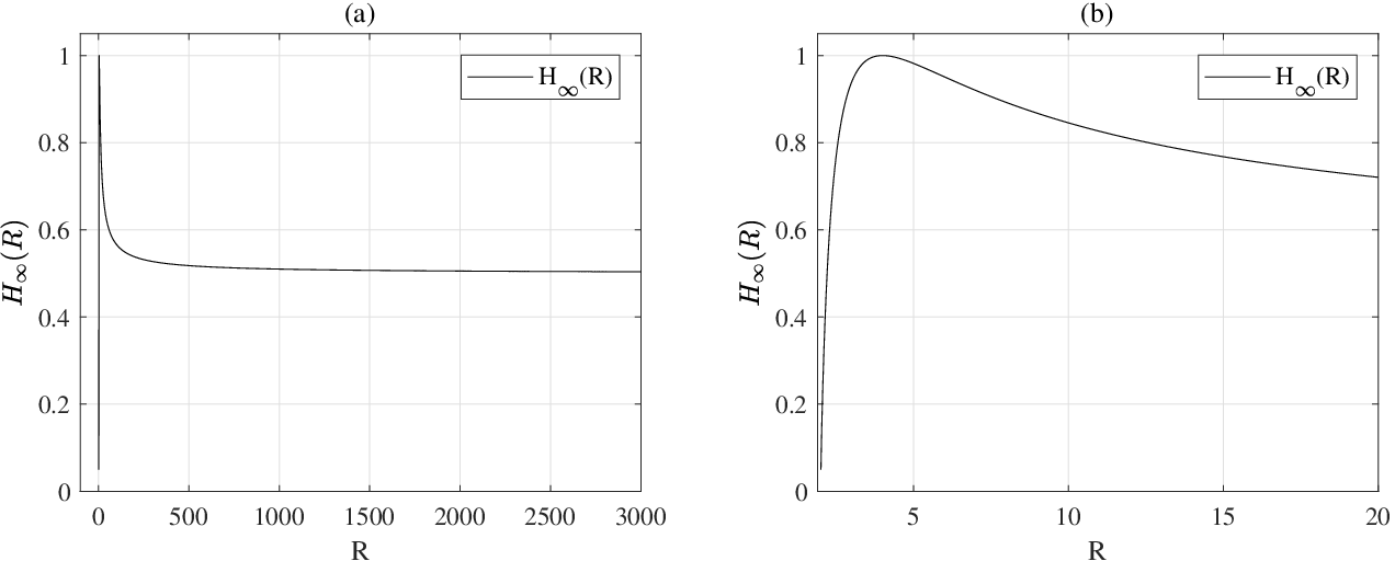
The proof of Theorem 1 is given in Section VI-E. In Figure 4 we depict the entropy rate $\mathscr{H}_{\infty}(R)$ for a range of values of $R$. The entropy rate is zero for $R=2$ because the dendritic structure of a perfect planted binary plane tree is predetermined for any $N$. Note that, when $R$ is allowed to grow, the entropy rate converges to $1/2$. More precisely,

Thus, for large $R$ and $N$ one would need about $N/2$ bits to decode the entire tree. It would be interesting to explain why trees with large enough $R$ require less bits to encode them than the trees with $R=4$.

For $R=4$ the entropy rate attains its maximal value $1$. Recall that the critical binary Galton-Watson model has parameter $R=4$. It was noticed that the Horton exponents for real rivers are different from the theoretical parameter $R=4$ [11]. For example, for Amazon river $R=4.51$. Consequently, entropy rate for Amazon river is $0.9941$. A natural question to ask would be: What physical phenomenon does cause the nonoptimality of entropy rate of the rivers? A possible explanation of this phenomenon is given in [38]: although river deltas adjust their configurations to maximize the entropy, this maximization happens within local feasibility constraints, thus global maximum is not achieved.

We begin with two auxiliary lemmas that will be used in the proof of Theorem 1.

References

- [1] D. Turcotte, B. Malamud, G. Morein, and W. Newman, “An inverse-cascade model for self-organized critical behavior,” Physica A: Statistical Mechanics and its Applications, vol. 268, no. 3, pp. 629–643, 1999.
- [2] D. K. Sorting, “Searching, the art of computer programming, vol. 3,” 1973.
- [3] G. Yakovlev, W. I. Newman, D. L. Turcotte, and A. Gabrielov, “An inverse cascade model for self-organized complexity and natural hazards,” Geophysical Journal International, vol. 163, no. 2, pp. 433–442, 2005.
- [4] I. Zaliapin, H. H. L. Wong, and A. Gabrielov, “Inverse cascade in a percolation model: Hierarchical description of time-dependent scaling,” Physical Review E, vol. 71, no. 6, p. 066118, 2005.
- [5] I. Zaliapin, H. Wong, and A. Gabrielov, “Hierarchical aggregation in percolation model,” Tectonophysics, vol. 413, no. 1, pp. 93–107, 2006.
- [6] I. Zaliapin and Y. Kovchegov, “Tokunaga and Horton self-similarity for level set trees of Markov chains,” Chaos, Solitons & Fractals, vol. 45, no. 3, pp. 358–372, 2012.
- [7] R. E. Horton, “Erosional development of streams and their drainage basins; hydrophysical approach to quantitative morphology,” Geological society of America bulletin, vol. 56, no. 3, pp. 275–370, 1945.
- [8] A. N. Strahler, “Quantitative analysis of watershed geomorphology,” Eos, Transactions American Geophysical Union, vol. 38, no. 6, pp. 913–920, 1957.
- [9] I. Yekutieli and B. Mandelbrot, “Horton-Strahler ordering of random binary trees,” Journal of Physics A: Mathematical and General, vol. 27, no. 2, p. 285, 1994.
- [10] R. Kemp, “The average number of registers needed to evaluate a binary tree optimally,” Acta Informatica, vol. 11, no. 4, pp. 363–372, 1979.
- [11] S. D. Peckham, “New results for self-similar trees with applications to river networks,” Water Resources Research, vol. 31, no. 4, pp. 1023–1029, 1995.
- [12] L. Devroye and P. Kruszewski, “A note on the Horton-Strahler number for random trees,” Information processing letters, vol. 52, no. 3, pp. 155–159, 1994.
- [13] W. Newman, D. Turcotte, and A. Gabrielov, “Fractal trees with side branching,” Fractals, vol. 5, no. 04, pp. 603–614, 1997.
- [14] D. Turcotte, J. Pelletier, and W. Newman, “Networks with side branching in biology,” Journal of Theoretical Biology, vol. 193, no. 4, pp. 577–592, 1998.
- [15] S. A. Veitzer and V. K. Gupta, “Random self-similar river networks and derivations of generalized Horton laws in terms of statistical simple scaling,” Water resources research, vol. 36, no. 4, pp. 1033–1048, 2000.
- [16] G. A. Burd, E. C. Waymire, and R. D. Winn, “A self-similar invariance of critical binary Galton-Watson trees,” Bernoulli, vol. 6, no. 1, pp. 1–21, 2000.
- [17] P. S. Dodds and D. H. Rothman, “Scaling, universality, and geomorphology,” Annual Review of Earth and Planetary Sciences, vol. 28, no. 1, pp. 571–610, 2000.
- [18] A. N. Strahler, “Hypsometric (area-altitude) analysis of erosional topography,” Geological Society of America Bulletin, vol. 63, no. 11, pp. 1117–1142, 1952.
- [19] B. T. Milne and V. K. Gupta, “Horton ratios link self-similarity with maximum entropy of eco-geomorphological properties in stream networks,” Entropy, vol. 19, no. 6, p. 249, 2017.
- [20] J. Neveu, “Erasing a branching tree,” Advances in applied probability, pp. 101–108, 1986.
- [21] P. S. Dodds and D. H. Rothman, “Unified view of scaling laws for river networks,” Physical Review E, vol. 59, no. 5, p. 4865, 1999.
- [22] D. G. Tarboton, R. L. Bras, and I. Rodriguez-Iturbe, “The fractal nature of river networks,” Water Resources Research, vol. 24, no. 8, pp. 1317–1322, 1988.
- [23] A. Gabrielov, W. Newman, and D. Turcotte, “Exactly soluble hierarchical clustering model: Inverse cascades, self-similarity, and scaling,” Physical Review E, vol. 60, no. 5, p. 5293, 1999.
- [24] Y. Kovchegov, I. Zaliapin, et al., “Horton self-similarity of Kingmans coalescent tree,” in Annales de l’Institut Henri Poincaré, Probabilités et Statistiques, vol. 53, pp. 1069–1107, Institut Henri Poincaré, 2017.
- [25] J. Pitman, Combinatorial Stochastic Processes: Ecole d’Eté de Probabilités de Saint-Flour XXXII-2002. Springer, 2006.
- [26] Y. Kovchegov and I. Zaliapin, “Horton law in self-similar trees,” Fractals, vol. 24, no. 02, p. 1650017, 2016.
- [27] R. L. Shreve, “Statistical law of stream numbers,” The Journal of Geology, vol. 74, no. 1, pp. 17–37, 1966.
- [28] T. M. Cover and J. A. Thomas, Elements of information theory. John Wiley & Sons, 2012.
- [29] C. E. Shannon, “A mathematical theory of communication,” Bell system technical journal, vol. 27, no. 3, pp. 379–423, 1948.
- [30] J. C. Kieffer, E.-H. Yang, and W. Szpankowski, “Structural complexity of random binary trees,” pp. 635–639, 2009.
- [31] S. Zanardo, I. Zaliapin, and E. Foufoula-Georgiou, “Are American rivers Tokunaga self-similar? New results on fluvial network topology and its climatic dependence,” Journal of Geophysical Research: Earth Surface, vol. 118, no. 1, pp. 166–183, 2013.
- [32] R. L. Shreve, “Infinite topologically random channel networks,” The Journal of Geology, vol. 75, no. 2, pp. 178–186, 1967.
- [33] R. E. Horton, “Drainage-basin characteristics,” Eos, transactions american geophysical union, vol. 13, no. 1, pp. 350–361, 1932.
- [34] J. W. Kirchner, “Statistical inevitability of Horton’s laws and the apparent randomness of stream channel networks,” Geology, vol. 21, no. 7, pp. 591–594, 1993.
- [35] D. G. Tarboton, “Fractal river networks, Horton’s laws and Tokunaga cyclicity,” Journal of hydrology, vol. 187, no. 1-2, pp. 105–117, 1996.
- [36] V. K. Gupta and E. C. Waymire, “Some mathematical aspects of rainfall, landforms, and floods,” in Stochastic Methods In Hydrology, pp. 129–171, World Scientific, 1998.
- [37] I. Rodriguez-Iturbe and A. Rinaldo, “Fractal river networks: chance and self-organization,” 1997.
- [38] A. Tejedor, A. Longjas, D. A. Edmonds, I. Zaliapin, T. T. Georgiou, A. Rinaldo, and E. Foufoula-Georgiou, “Entropy and optimality in river deltas,” Proceedings of the National Academy of Sciences, 2017.